Sage Journals: Discover world-class research

Abstract

Standing at 24% in 2018, India’s female labour force participation is only half of the global average (48%). At the same time, India has one of the widest gender wage gaps in the world and women are less likely to be employed in the formal sector compared to men. This article focuses on how international trade affects relative wages and formal employment between men and women in India. Using the Revealed Symmetrical Comparative Advantage index, sectors of comparative advantage and disadvantage are identified and matched to Indian labour force surveys that contain information on sectoral employment and earnings. We find that sectors of comparative advantage in services have the lowest gender wage gap, with women earning 24% less than their male counterparts, while women in manufacturing earned on average 40% less than male workers. Using the Oaxaca–Blinder decomposition, we find that the total gender wage gap in sectors of comparative advantage in services are minor while it is quite substantial in manufacturing, regardless of comparative advantage status. The article concludes that services trade goes hand in hand with a smaller gender wage gap as women leverage their skills better in services than in manufacturing.

JEL Codes: F16, F14

Keywords

Gender services trade jobs earnings

Introduction

Over the past few decades, India has made strides in narrowing the gender wage gap. The difference in average pay between men and women as a share of average men’s wage has come down from 48% in 1993–1994 to 34% in 2011–2012 (ILO, 2018). Standing at 29% in 2017, India has one of the lowest female labour force participation rates in the world. For comparison, the female participation rate was 69% in China, 66% in USA and 57% globally.¹ Furthermore, only around 9% of employment in India is salaried or regular jobs, and of those, women hold 18%.

During the past few decades, India has also become one of the major services exporters in the world. This article analyses a possible connection between the rise of India’s services exports and the narrowing of the gender wage gap. For benchmarking and comparison, we analyse the manufacturing sector on the same metrics as services.

There are three main channels through which trade may affect women’s employment and wages. First, if sectors of comparative advantage employ relatively more women, women may gain from trade and trade liberalisation (Nordås, 2003). Second, in a setting of heterogenous firms and entry costs in foreign markets, the smallest and least productive firms will exit the market and the largest and most productive firms will expand and export in the event of trade liberalisation (Melitz, 2003; Nataraj, 2011). If women are more likely to work in small and less productive firms, they will lose from trade. Both these channels affect women through pre-existing biases and do not necessarily imply discrimination of women in the sector or firm they work in.

The third channel operates through raising the cost of discrimination. If trade put firms’ profit margins under pressure, they would look for ways to cut costs. Gender discrimination may contribute to higher unit labour costs, which firms can no longer afford in the face of stronger competition (Becker, 1971).

Given India’s industrial structure and gender composition of employment, one would expect that women gain through the first and third channel but may lose from the second. However, our analysis finds that although women’s share of employment is higher than average in textiles, clothing and chemicals, which are sectors of revealed comparative advantage (RCA), the relationship between comparative advantage and gender shares in employment is not strong. The first channel thus appears not to be important. We also found no systematic gender differences in the composition of employment by firm size, at least for the size categories available in the data. We are then left with the cost of discrimination as the main channel through which trade could affect the gender wage gap.

Our main source of data is the Indian National Sample Survey (NSS) Employment and Unemployment Survey for the years 2000, 2005, 2010 and 2012. These surveys provide rich information on worker-level characteristics, daily wages, sector of employment and geographic location. Using trade data from World Input–Output Database (WIOD), we calculate revealed symmetrical comparative advantage (RSCA). With this information at hand, we can trace employment patterns by gender, and by sectors of comparative advantage and disadvantage.

The econometric analysis starts with a baseline ordinary least squares (OLS) estimation of the relationship between wages and gender, controlling for relevant individual characteristics. We find that the smallest gender wage gap is in services sectors with relatively strong RSCAs where women earn 24% less than their male counterpart. For comparison, women in manufacturing sectors of comparative advantage earned on average 42% less than male workers.

We next apply an Oaxaca–Blinder decomposition which allows the explanatory variables to have a different marginal effect on wages for men and women. This almost eliminates the gender wage gap in services sectors of comparative advantage while the gap remains substantial in manufacturing, regardless of comparative advantage status. The decomposition further indicates that women may be over-qualified for their jobs, which is a common strategy to circumvent a biased labour market (Blau & Kahn, 2017).

The rest of the article is organised as follows: Section 2 positions the article in the current literature. Section 3 describes the data and variables used in the descriptive statistics and subsequent regression analysis. Section 4 presents the ranking of sectors according to the RSCA index and its developments over time while Section 5 presents employment patterns and wages by RSCA category and gender. Section 6 relates the gender wage gap to the sector of employment’s comparative advantage using an Oaxaca–Blinder decomposition. Finally, Section 7 summarises and concludes.

Relations to Previous Research

The first wave of globalisation starting in the 1960s involved an expansion of export-oriented labour intensive manufacturing industries in developing countries. Thus, trade liberalisation created jobs in textiles, toys and similar industries, which tend to employ women. Such effects were for instance recently found for Indonesia (Kis-Katos et al., 2018). However, with the industrial upgrading to more sophisticated products and more skill-intensive jobs, women’s relative gains levelled off globally.²

India opened up to international trade somewhat later than the Southeast Asian economies and did not embark on an export-led industrialisation process. The country thus did not experience a female employment boom similar to that observed first in South Korea and later in China, Vietnam and Bangladesh. Nevertheless, a similar pattern was later observed for services. Information and communication technology-enabled back office jobs were largely filled by women, including in call centers servicing foreign clients (World Bank, 2012). Since services sectors in general tend to employ women intensively, our finding that there is no systematic relationship between comparative advantage and female share of employment in India is not surprising.

Turning to the cost of discrimination channel, the seminal work on the economics of discrimination by Becker (1971) inspired a growing literature estimating and explaining the difference in wages between equally productive men and women. Black and Brainerd (2004) supported Becker’s theory in a study of US manufacturing. They found that trade liberalisation increased competitive pressure, which subsequently reduced the gender wage gap. A comprehensive review of the literature in 2005 (Weichselbaumer & Winter-Ebmer, 2005) found that the mean unexplained gender wage gaps reported in the reviewed studies were on average about 23% in the 1960s compared to 19% in the 1990s. The total gender wage gap, in contrast, came down by half (from 51% to 26%) during the same period as women caught up on education, training and experience. The literature consistently finds a lower wage gap in the public sector and the wage gap is larger for married employees.³

Early work following the cost of discrimination hypothesis implicitly assumed that men and women are inherently perfect substitutes in the labour market. Thus, wages were regressed on a gender dummy controlling for different levels of education, age, experience and other personal characteristics, implying that the confounding variables have the same marginal impact on wages for men and women. Questioning this assumption, Oaxaca (1973) suggested a decomposition of the gender wage gap in an explained and an unexplained (residual) part where the latter is considered to be due to discrimination (Juhn et al., 2014).

The residual gender wage gap is not uniform across the wage distribution. If the wage gap is higher at the top of the income distribution, a glass ceiling may be present. Conversely, a wider wage gap at the bottom of the distribution indicates a sticky wage floor. Glass ceilings are more common in developed countries, while sticky floors are mainly found in developing countries (ILO, 2018). In India, the gender wage gap declines from about 60 percentage points at the lowest income levels to about 40 points at the 40th percentile, and then rises back to more than 60 percentage points at the 75th percentile after which it drops sharply to 13 percentage points at the top income level, indicating a sticky floor (Duraisamy & Duraisamy, 2016).

Studies on trade and the gender wage gap in India largely investigate the cost of discrimination channel using the Oaxaca–Blinder composition. Chamarbagwala (2006) found a widening skills wage gap and a narrowing gender wage gap following economic liberalisation from the 1960s to the late 1980s. Trade liberalisation in manufacturing benefited skilled men and hurt skilled women, while services offshoring benefitted college graduates of both sexes. Menon and van der Meulen Rodgers (2009) focussed on manufacturing and found that more competitive pressure from trade in sectors that faced little domestic competition before trade liberalisation was associated with a widening gender wage gap. Finally, Dutta and Reilly (2008) studied sector-level gender wage gaps and found that the residual gender wage gap had little to do with openness to trade. If anything, trade had a benign effect on the gender wage gap.

This article contributes to the literature in several ways. First, it includes both manufacturing and services and updates previous studies, which draw on data from the 1980s and 1990s. Second, our trade variable, RSCA, captures the underlying relationship between trade and wages as spelled out by the Stolper–Samuelsson theorem. Sectors of comparative advantage are expected to expand and hire while the relative wage of the factor used intensively in the sector is expected to rise in the event of trade liberalisation. Conversely, sectors of comparative disadvantage are expected to contract, lay off workers and the relative wage of the factor used intensively in the sector is expected to decline in the event of trade liberalisation. Expanding sectors may be less concerned with cost cutting than contracting sectors. Hence, sectors of comparative disadvantage may be more inclined to eliminate costly discrimination. Our methodology sheds light on this question and thus also whether gender wage discrimination is more affordable in industries facing import competition compared to industries facing export competition.

Data

The NSS, headed by the National Sample Survey Office, collects employment and activity information from a large sample of households, from each of the 29 states and 7 union territories of India. The survey is conducted every five years from 1972 and onwards. This article uses four waves: 50th (1993–1994), 55th (1999–2000), 61st (2004–2005) and 68th (2011–2012). The main outcome variable of interest is the female-to-male wage ratio by two-digit industries according to the National Industry Classification (NIC). Several data issues are worthy of note. See Table A1 for descriptive statistics.

First, the variable used to identify an individual’s activity status, and subsequently the wage rate, refers to a specific reference week, and not the total for the past year.⁴ Second, around 11% of the individuals who reported additional subsidiary activities were excluded in the analysis since it would be impossible to disentangle sector-specific effects on wages for these individuals Third, because individuals divide their time across several activities, total wage and salary earnings were normalised using daily wage rates to achieve comparability. Fourth, rather than deflating nominal wages, we used time-fixed effects. Fifth and lastly, during the period of analysis, the NIC was updated two times: 2004 and 2008. Although the NIC exists at the five-digit level, it is not possible to do a perfect conversion between the classifications at that level. Therefore, the analysis is conducted at the two-digit level, where there are 56 industries in the sample. This classification also corresponds to the WIOD 2016 release which is the source of trade statistics (Timmer et al., 2015).

India has eight years of compulsory schooling between the ages of 6 and 14. In the empirical analysis, we aggregated the initial 14 levels of education into 3: below secondary, upper secondary and tertiary education. The latter includes both university and technical (vocational) education. Household size is the number of individuals that lives in the same household as the participant. Married status is a binary variable where non-married individuals include those who have never been married, widows/widowers and divorced/separated.

Occupations are reported as an individual’s main activity during the reference week and are classified according to the National Classification of Occupations (NCO) at the three-digit level. Approximately, 57% of observations are categorised under an older NCO classification (1968) while the more recent from 2004 applies to the rest (43%). In the older classification, there were 460 occupation categories at the three-digit level, while there are 114 occupation groups in the newer classification (2,498 occupations at the six-digit level). Unfortunately, harmonisation across the older and newer NCO is impossible. For this reason, all occupations are re-classified into seven broad occupational divisions (see Table A3). About 9% of the observations had to be dropped because occupations could not be classified reliably.

Sectors in the Indian Labour Force Survey are classified according to the National Industrial Classification (NIC) 2004 and 2008, which was then broadly divided into manufacturing and commercial services (henceforth services). Consequently, industries in agriculture and public services such as waste collection, utilities and public administration (including defence) were excluded from the final sample, which cover around 50% of workers in India (see Table A2).

Revealed Symmetrical Comparative Advantage

To identify sectors of comparative advantage, RCA is computed for each sector as follows: the numerator is total Indian exports in sector, i as a share of total Indian exports across all sectors. The denominator is world exports in sectors i, wⁱ, as a share of total world exports (W) across all sectors.

R C A = \frac{x^{i} / X}{w^{i} / W}

As is standard, the RCA is adjusted to become symmetric around zero, giving RSCA. An RSCA value of zero would represent a situation where the country’s export share is identical to the world total export share for this sector (Laursen, 2015).

R S C A = \frac{R C A - 1}{R C A + 1}

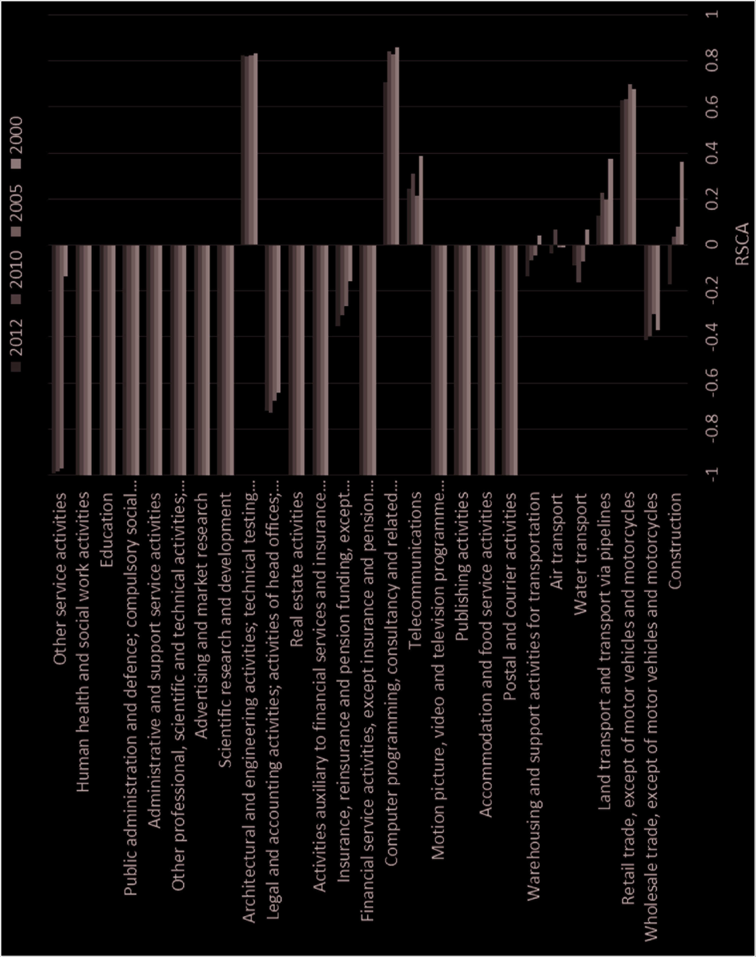
Figures 1 and 2 present the RSCA index for one- and two-digit industry codes (NACE) in goods and services respectively, which were calculated using WIOD. India’s comparative advantage in services lies mainly in architecture and engineering, computer programming, retail trade and land transport, while in manufacturing, comparative advantage is the strongest in chemicals, coke and refined petroleum products, basic metals, furniture and textiles. We also note that India has a strong revealed comparative disadvantage in the manufacture of computer, electronic and optical products and that for most services a strong revealed comparative disadvantage is observed. Thus, India has RCA in a narrow set of sectors, including business services.

Figure 1.

Source: World Input–Output database.

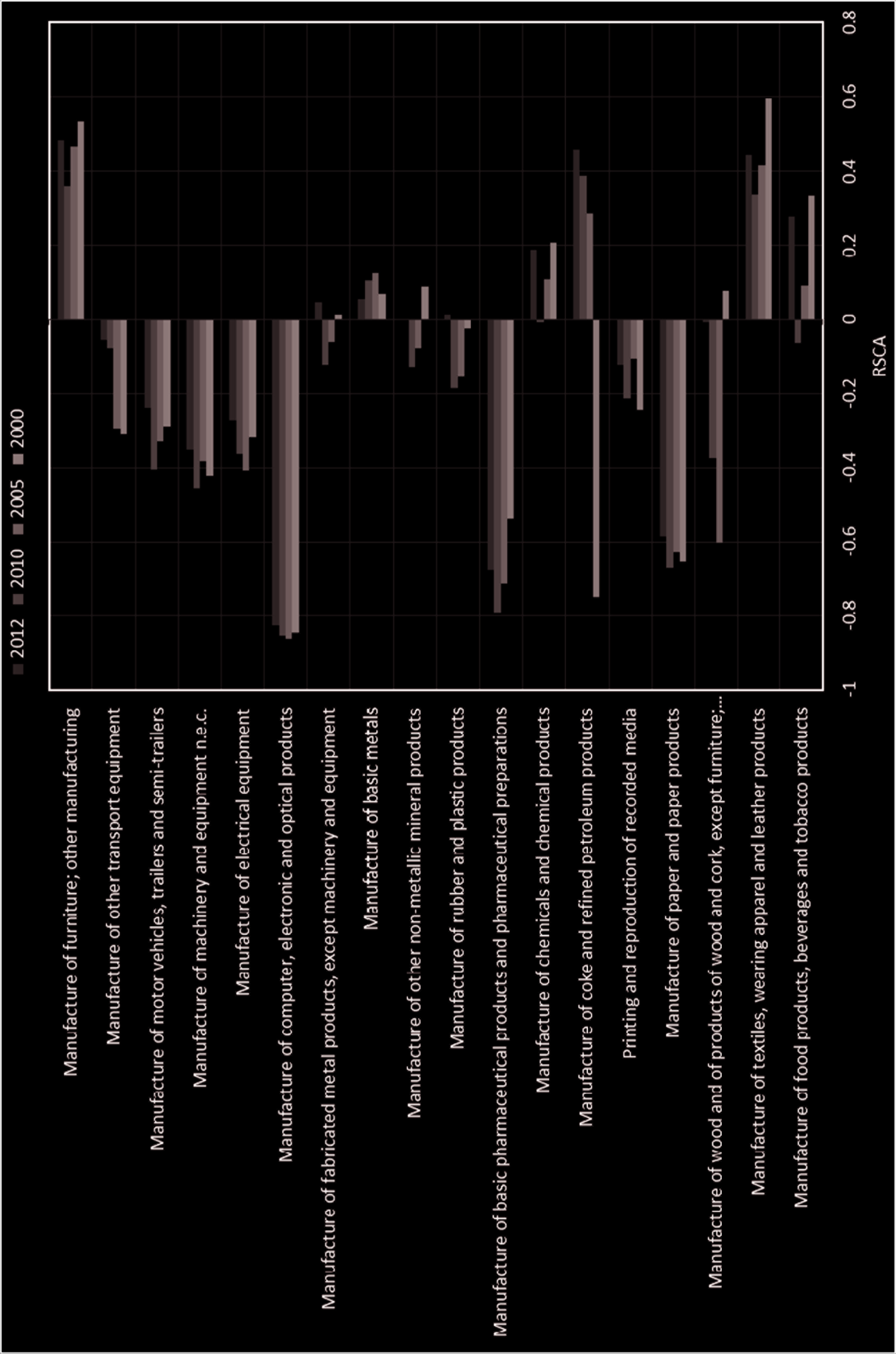
Figures 1 and 2 also reveal that over time, some sectors change from having comparative advantage to comparative disadvantage and vice versa. For example, manufacture of motor vehicles, trailers and semi-trailers as well as manufacture of coke and refined petroleum products has revealed stronger comparative advantage over time. Nevertheless, comparative advantage and disadvantage, overall, appears to have been relatively stable over a 12-year period.

Figure 2.

Source: World Input–Output database.

Descriptive Statistics

This section presents descriptive statistics for some key variables: wages, share of female workers, higher education, and formal employment. Note that, although the RSCA index is a continuous measure with cardinal properties, it will only be used here to identify which sectors have comparative advantage or disadvantage as it has poor ordinal ranking properties (Yeats, 1985).

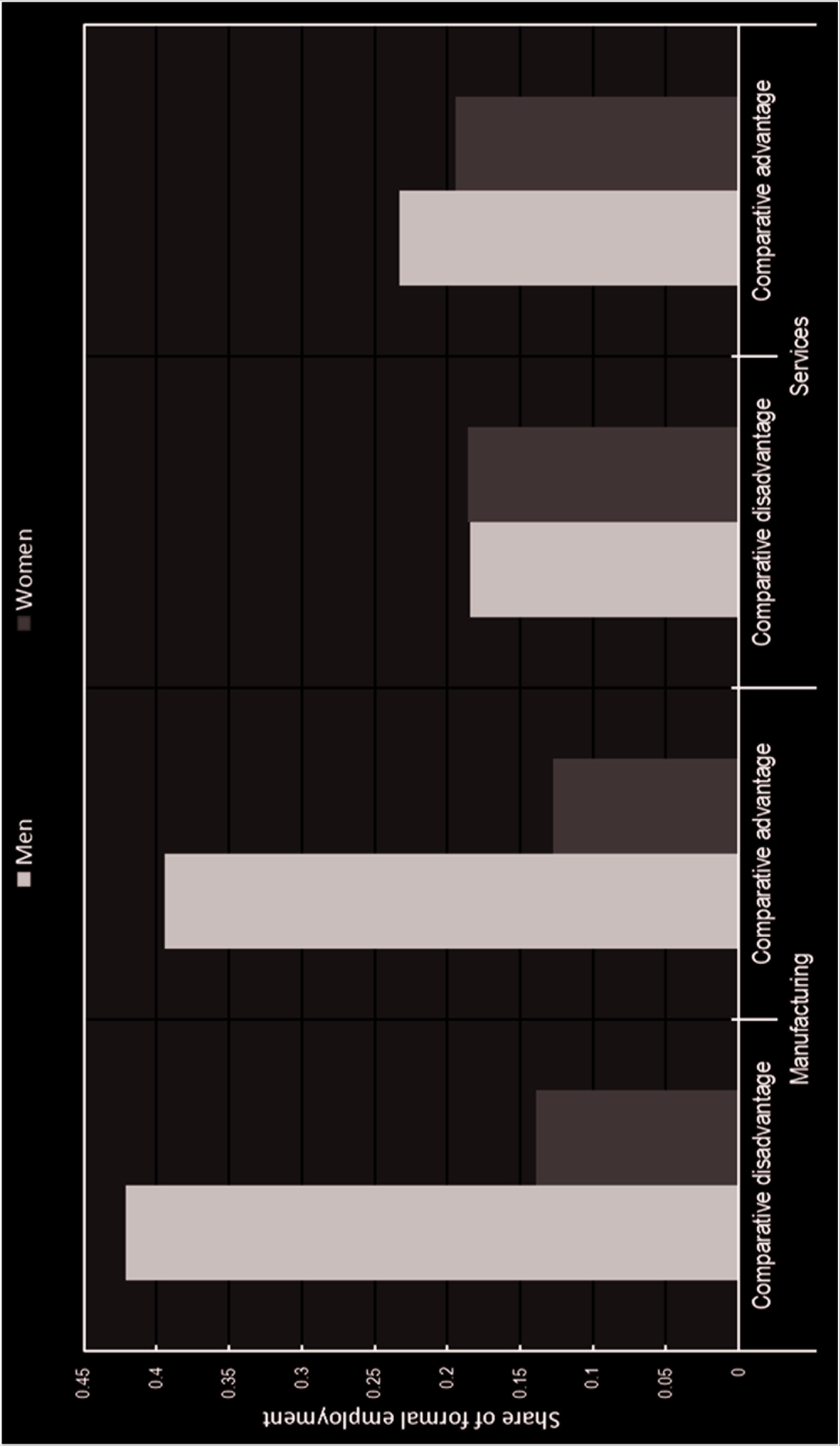
Figure 3 shows the distribution of male and female workers across broad economic sector and comparative advantage. Almost 75% of men work in services, while women are distributed equally between manufacturing and services. The largest gender difference is found in sectors of comparative advantage in manufacturing where 37% of women work, compared to 15% of men. This most likely reflects India’s considerable textile industry (see Figure 1).

Figure 3.

Source: Indian Labour Force Survey, 2000, 2005, 2010 and 2012.

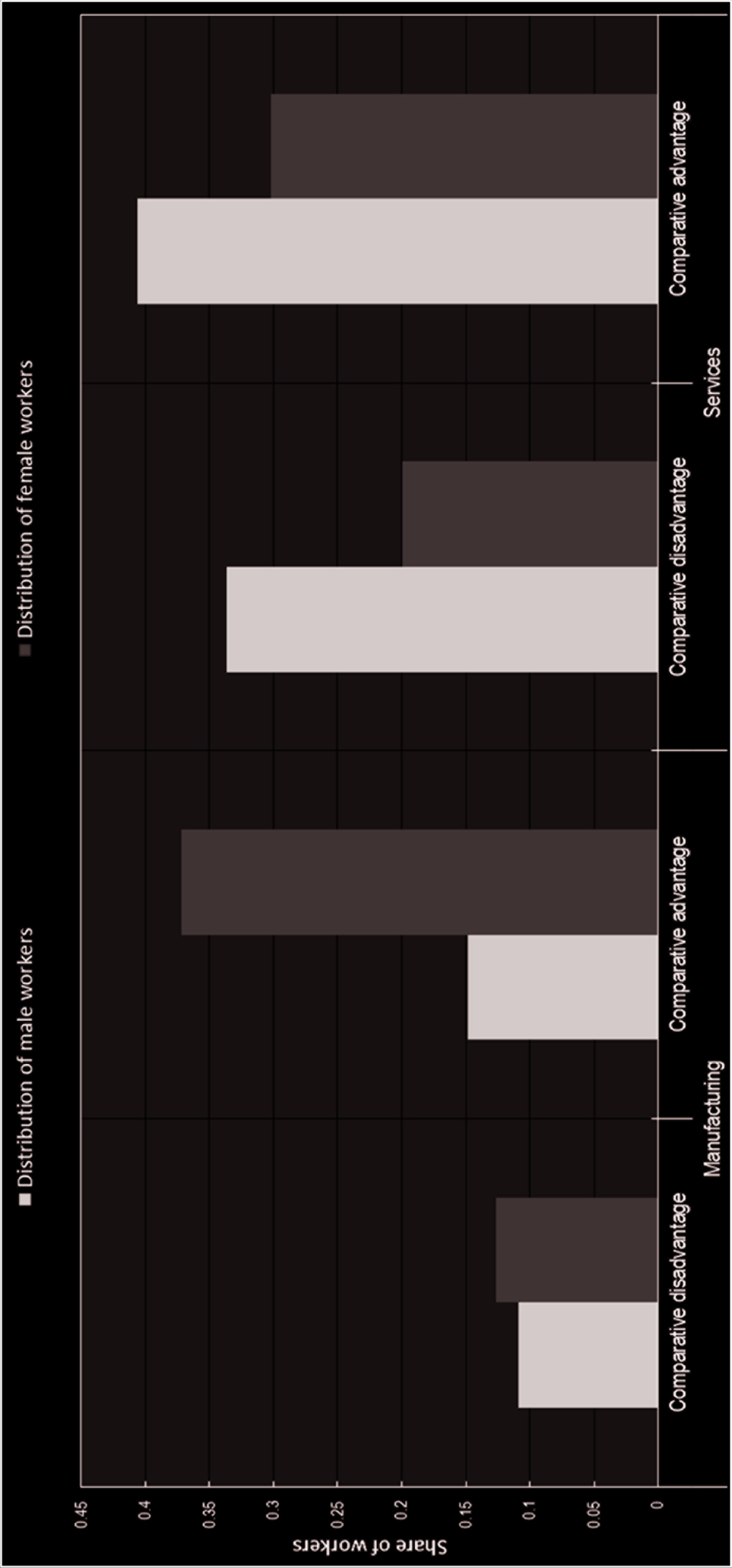
Figure 4 reports the average wage of women relative to the average wage of men by broad sector and comparative advantage. It shows that the female-to-men wage ratio is the highest in services sectors, and in sectors of comparative advantage in particular, where women earn around 90% of male wages. Women’s average wages, relative to men, are the lowest in manufacturing sectors with comparative advantage, where women earn 70% of male wages.

Figure 4.

Source: Indian Labour Force Survey, 2000, 2005, 2010 and 2012.

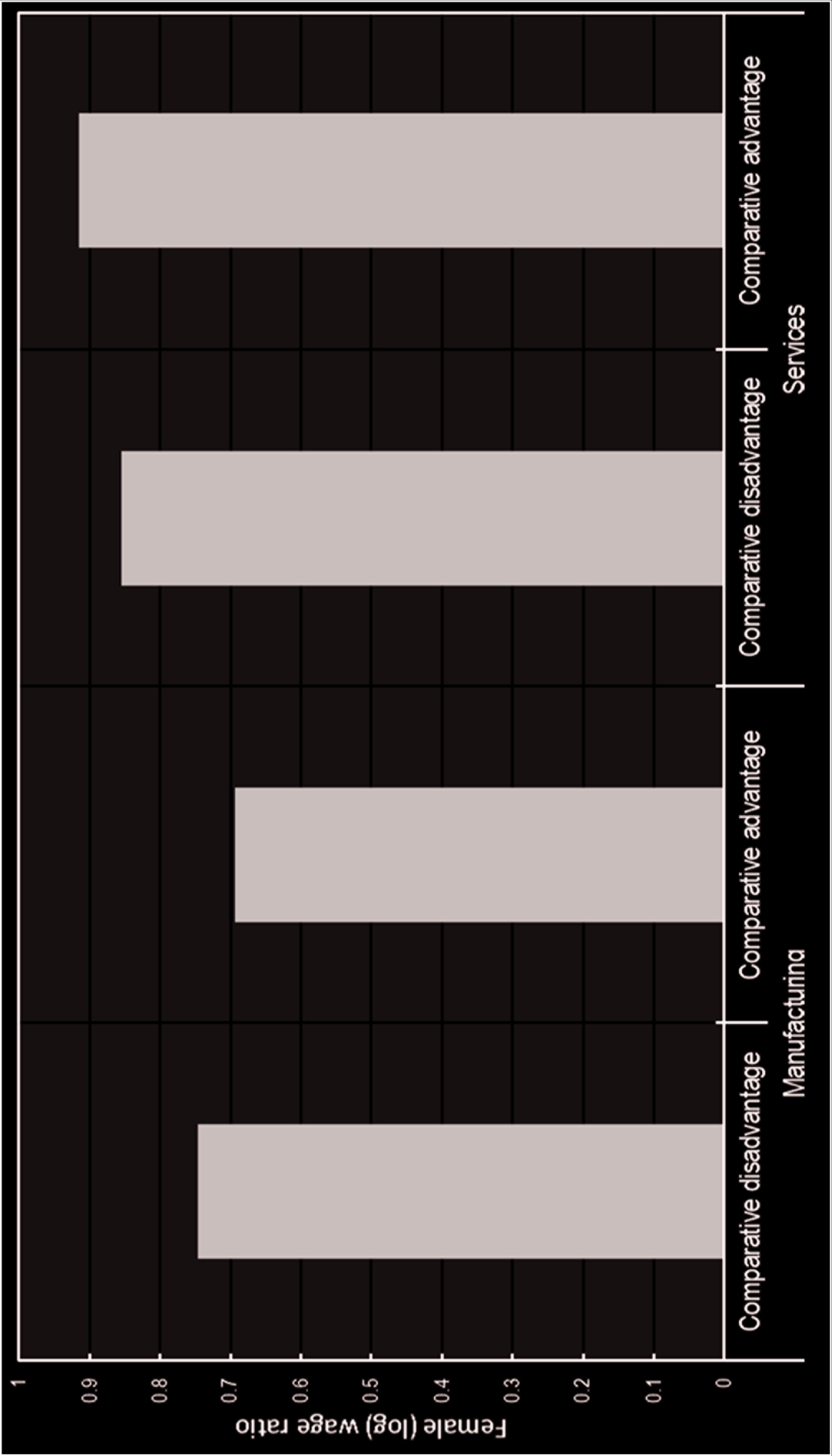
Figure 5 plots the share of workers in formal employment by gender and sectors. The largest imbalance is in manufacturing where around 40% of men are formally employed, compared to only 13%–14% for women. Women are better off in services where around 20% are formally employed with little to no difference between men and women.

Figure 5.

Source: Indian Labour Force Survey, 2000, 2005, 2010 and 2012.

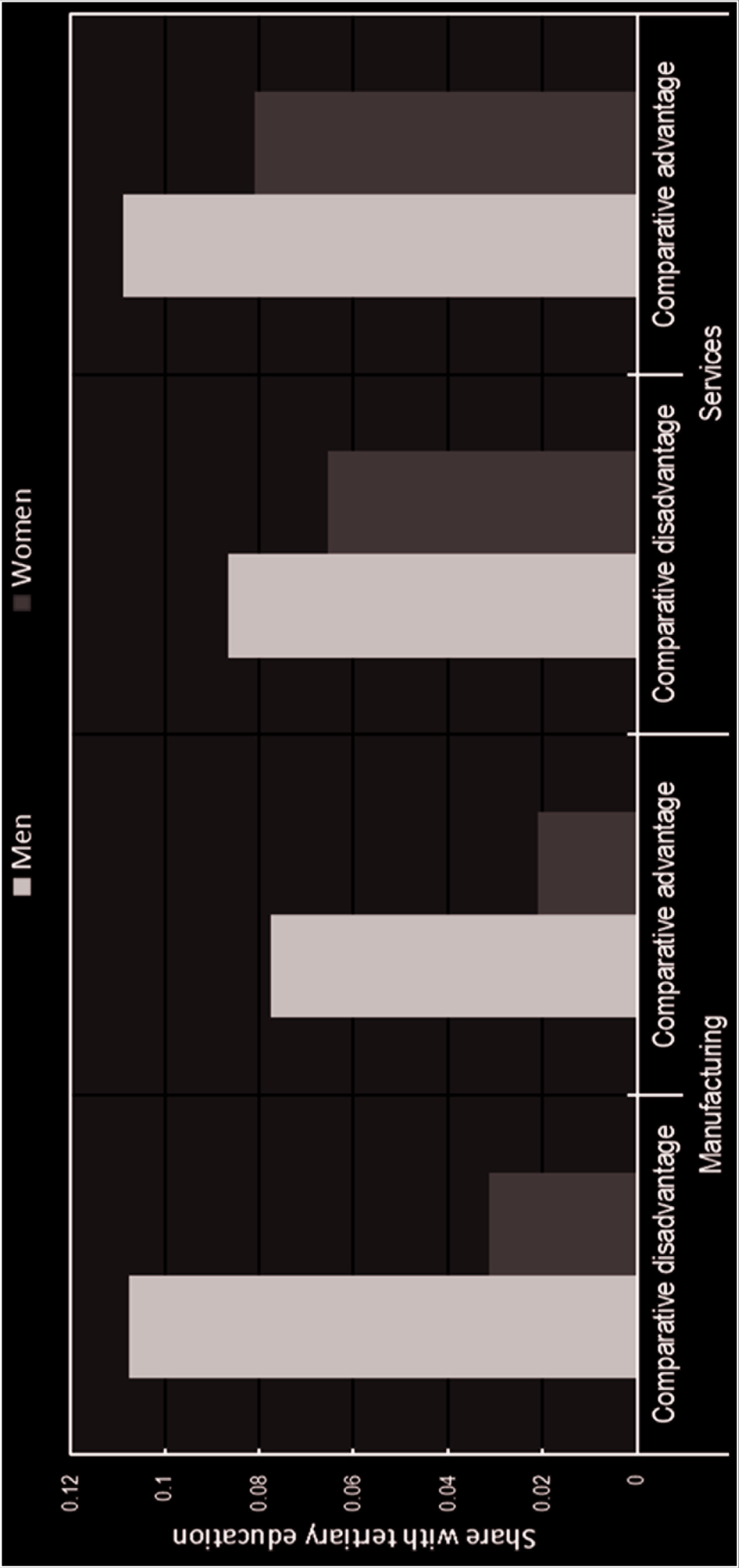
The higher female-to-male wage ratio reported for services in Figure 4 could reflect a smaller skills gap in services. In Figure 6, the share of workers with tertiary education is clearly the highest in services sectors of comparative advantage, with around 11% men and 8% women with higher education. Again, the largest gender discrepancy is found in manufacturing where sectors of comparative disadvantage have 11% men with tertiary education compared to only 3% of the women.

Figure 6.

Source: Indian Labour Force Survey, 2000, 2005, 2010 and 2012.

To summarise the descriptive statistics, women are doing relatively better in services than in manufacturing on all the metrics considered. Interestingly, women are doing relatively better in the sectors of comparative disadvantage in manufacturing and the sectors of comparative advantage in services. Thus, to the extent that gender differences stem from discrimination, it is less affordable for importcompeting industries in manufacturing, as expected. For services, in contrast, export competing industries appear to be the sectors that can least afford discrimination.

Explaining the Gender Wage Gap

Descriptive statistics on the gender wage gap and formal employment are informative but does not explain the differences. To uncover a gender wage gap taking into account wage-setting factors such as level of education, experience and other individual characteristics, we estimate a wage equation using OLS. The baseline specification captures the simple difference between men and women through a dummy variable denoted by F and is specified as follows:

W_{i, k} = γ F_{i, k} + x_{i, k} β_{k} + ε_{i, k .}

For each individual i in sector k, the outcome variable W is the daily wage rate, in logs.⁵ A vector of wage-setting predictors, x, is included to control for factors such as age (linear and quadratic), education levels (no education, primary, upper secondary and tertiary), household size, area (urban or rural), marital status (married or not) and occupation. The error term is assumed to be normally distributed, E(ε_i,k) = 0. The model also accounts for regional differences between the 35 states and union territories of India.⁶ This equation is estimated separately for manufacturing and services and, further by comparative advantage or disadvantage.

The simple OLS approach assumes that the return-to-wage-determining variables are the same for men and women. To further examine the gender wage gap, this assumption is relaxed. For example, tertiary education may not give rise to the same job and wage opportunities for women as for men. A common method for explaining differences in the mean outcome of a variable between two groups is the Oaxaca–Blinder decomposition (Oaxaca, 1973). For each group, in this case men and women, a separate wage-setting equation is estimated, where the resulting wage difference is referred to as the residual wage gap.

The wage gap is estimated by using the coefficients in the men’s wage equation in the women’s wage equation, to generate women’s counterfactual wages. That is, the wage women would have received if women’s wages were determined in the same way as men’s wages. The wage gap is then decomposed into three sources: (a) Differences in wage-determining variables, or endowments, between men and women. (b) gender differences in the returns to these variables, referred to as coefficient effects. Significant gender differences in coefficients are commonly interpreted as gender discrimination. Note, however, that this second part of the wage gap should be interpreted with caution as the empirical model may not fully capture all relevant factors that explain received wages. (c) An interaction effect that considers the additional impact when there are differences in observable variables combined with differences in their returns on wages. The Oaxaca–Blinder decomposition of the expected wage difference between men and women is thus decomposed as follows:

D = \underset{E n d o w m e n t}{\underset{︸}{[E (X_{m}) - E (X_{f})]^{'} β_{m}}} + \underset{C o e f f i c i e n t}{\underset{︸}{E (X_{f})^{'} (β_{m} - β_{f})}} + \underset{I n t e r a c t i o n}{\underset{︸}{[E (X_{m}) - E (X_{f})]^{'} (β_{m} - β_{f})}}

Lastly, it should be noted that the sample includes employed persons only. In India, as in many developing countries, there is a high probability that an individual is employed, given that the individual is part of the labour force. However, the low female labour force participation rate in India means that the regression results stem from the relatively small group of working women.

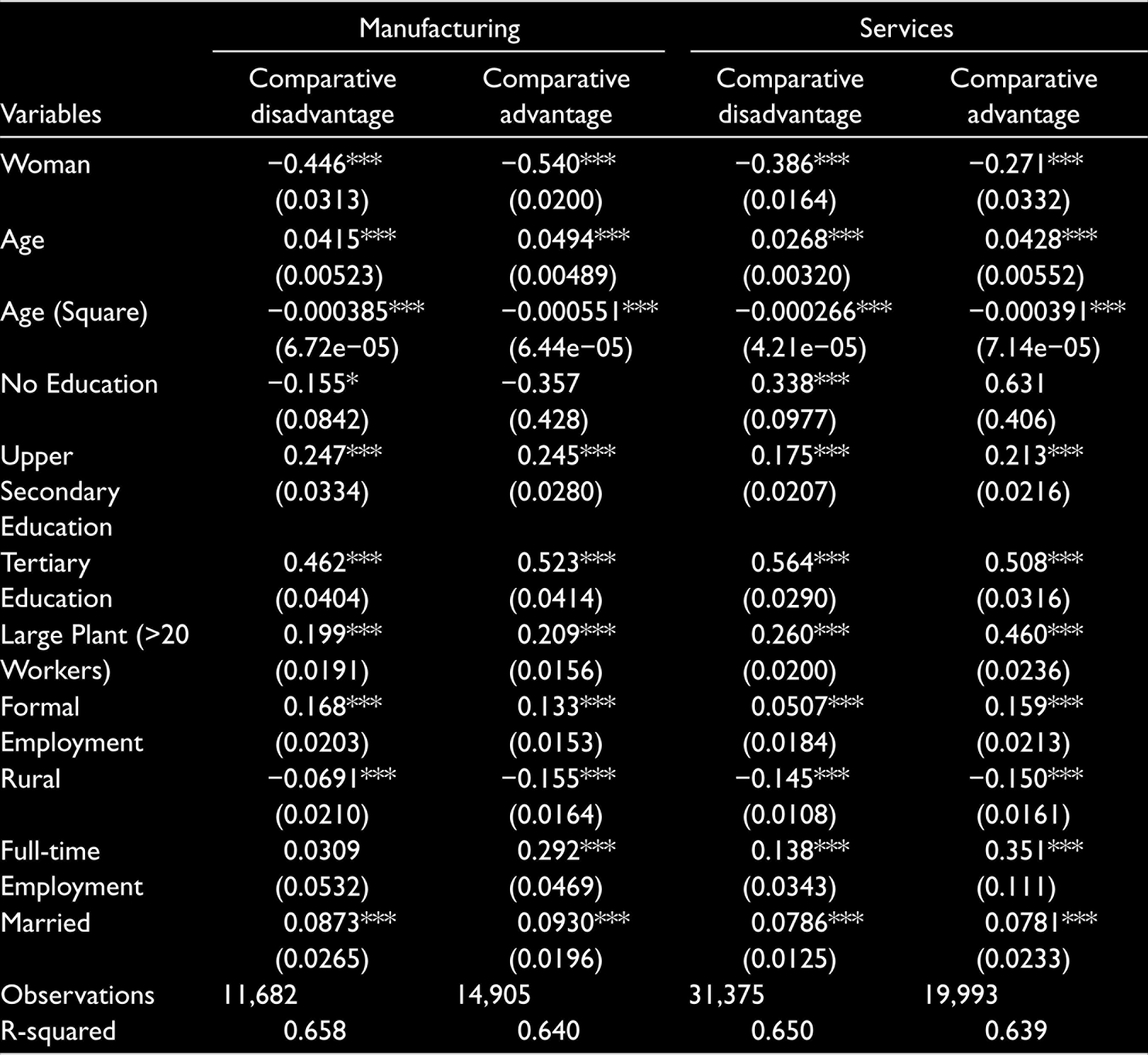
Table 1 presents the results of the baseline OLS regression of the gender wage gap. By including a gender variable in the model (first row), it measures the wage difference between men and women, controlling for differences in wage-determining factors such as education, assuming that all control variables have the same marginal effect on men and women’s wages. The average pay gap in manufacturing is estimated at around 42% lower wages for women in sectors of comparative advantage and 35% in sectors of comparative disadvantage. For services, the wage gap is about 24% for sectors of comparative advantage and 32% for sectors of comparative disadvantage.⁷

Table 1.

Robust OLS Regressions with Fixed Effects, Gender Wage Gap.

Variables	Manufacturing		Services
Variables	Comparative disadvantage	Comparative advantage	Comparative disadvantage	Comparative advantage
Woman	−0.446***	−0.540***	−0.386***	−0.271***
	(0.0313)	(0.0200)	(0.0164)	(0.0332)
Age	0.0415***	0.0494***	0.0268***	0.0428***
	(0.00523)	(0.00489)	(0.00320)	(0.00552)
Age (Square)	−0.000385***	−0.000551***	−0.000266***	−0.000391***
	(6.72e−05)	(6.44e−05)	(4.21e−05)	(7.14e−05)
No Education	−0.155*	−0.357	0.338***	0.631
	(0.0842)	(0.428)	(0.0977)	(0.406)
Upper Secondary Education	0.247***	0.245***	0.175***	0.213***
Upper Secondary Education	(0.0334)	(0.0280)	(0.0207)	(0.0216)
Tertiary Education	0.462***	0.523***	0.564***	0.508***
Tertiary Education	(0.0404)	(0.0414)	(0.0290)	(0.0316)
Large Plant (>20 Workers)	0.199***	0.209***	0.260***	0.460***
Large Plant (>20 Workers)	(0.0191)	(0.0156)	(0.0200)	(0.0236)
Formal Employment	0.168***	0.133***	0.0507***	0.159***
Formal Employment	(0.0203)	(0.0153)	(0.0184)	(0.0213)
Rural	−0.0691***	−0.155***	−0.145***	−0.150***
	(0.0210)	(0.0164)	(0.0108)	(0.0161)
Full-time Employment	0.0309	0.292***	0.138***	0.351***
Full-time Employment	(0.0532)	(0.0469)	(0.0343)	(0.111)
Married	0.0873***	0.0930***	0.0786***	0.0781***
	(0.0265)	(0.0196)	(0.0125)	(0.0233)
Observations	11,682	14,905	31,375	19,993
R-squared	0.658	0.640	0.650	0.639

Source: Indian Labour Force Survey, 2000, 2005, 2010 and 2012.

Notes: Fixed effects include industry, year, occupations, state, household size, and land ownership. Robust standard errors in parentheses ***P < .01, **P < .05, *P < .1.

Dependent variable: log hourly wage.

Age, rural areas, and marital status have a relatively small effect on wages, though they are statistically significant. Tertiary education is, as expected, highly influential in determining wages in all sectors, with those workers earning around 67% higher wages compared to those with only primary education (the reference category). Having a full-time job matters most in comparative advantaged sectors across both manufacturing and services, with such workers receiving around 30%–40% higher wages than those on other types of contracts (part-time or fixed-term contracts). Plant size has a substantial effect on wages in services sectors of comparative advantage, where workers in large plants (above 20 employees) on average earn 60% higher wages than those in smaller plants. Workers in formal employment have around 20% higher wages, except in services sectors of comparative disadvantage, where formal employment appears to have minor influence on wages.

We next relax the assumption of gender-neutral marginal effects of wage-determining factors by using the Oaxaca–Blinder method. In Figure 7, we present the results graphically, while the regression results are reported in Table A4.

Figure 7.

Source: Authors’ estimates based on Indian Labour Force Survey, 2000, 2005, 2010 and 2012.

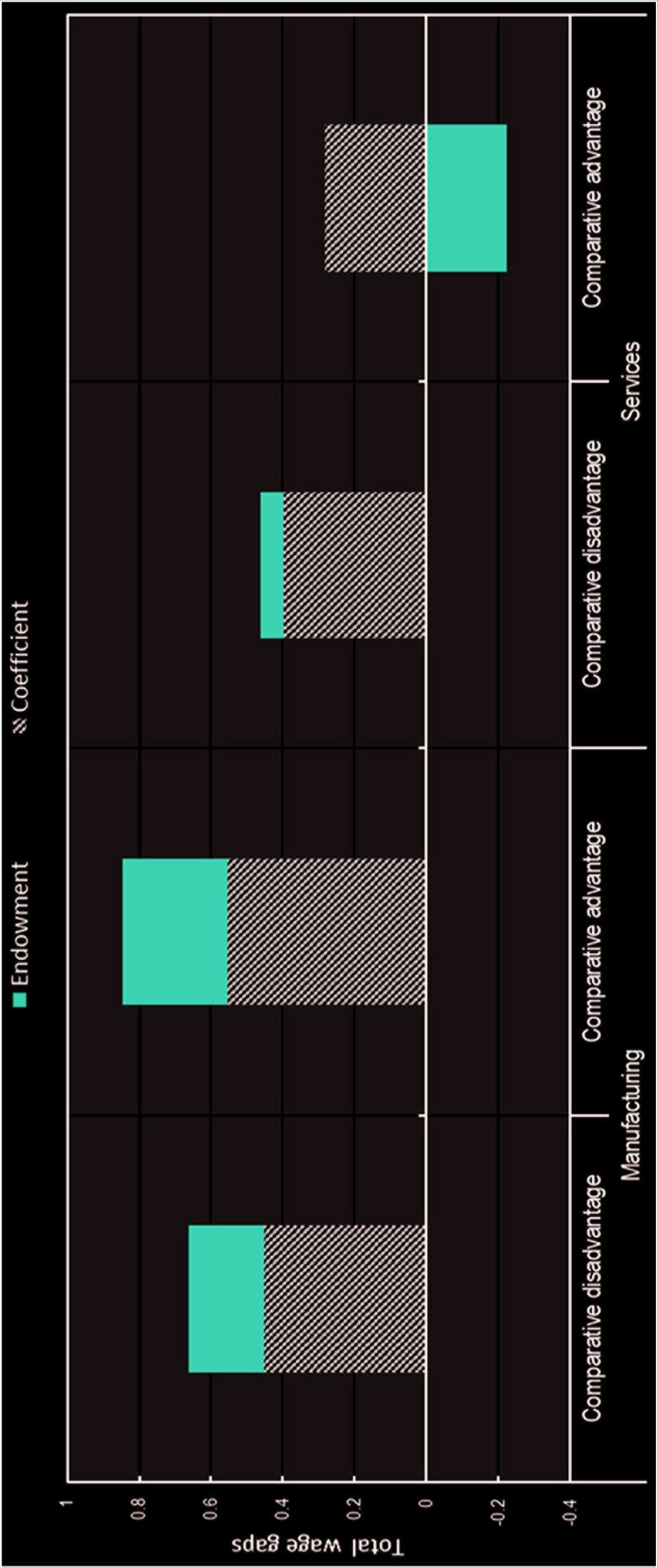
Figure 7 presents the decomposition of the total wage gap into endowment and coefficient effects. The endowment effect captures the part of the gender wage gap that is explained by differences in individual features such as age, education and the other confounding factors included in the regression. The coefficient effect captures the different returns to these features for men and women and thus the residual or unexplained part.

Figure 7 reveals some interesting features. First, the wage gap that can be explained by endowments is relatively small in all sector groups and particularly in services. Thus, gender biases in some shape or form appear to account for most of the gender wage gap in India. Second, although the wage gap is much larger in manufacturing, endowments explain more of it in manufacturing than in services.

Interestingly, there is a negative endowment effect in service sectors of comparative advantage. That means that women in this category are better endowed than men, which would have resulted in women earning 20% higher wages than men on average if the returns to observable wage-determining variables were the same. As we can see from the regression results depicted in Table A4, tertiary education accounts for the bulk of the endowment effect, followed by the combination of formal employment in large firms in urban areas. Even if the coefficient effect, which hints at discrimination, accounts for a larger part of the wage gap in services, it is still smaller in absolute terms than in manufacturing.

In manufacturing, women are on average both less endowed and obtain smaller returns on their endowments than men. The coefficient effect is highest in manufacturing of comparative advantage, which supports the expectation that contracting sectors can ill afford costly discrimination. In services, in contrast, the coefficient effect is smaller in sectors of comparative advantage, contrary to expectations. However, this could be explained by the fact that services exporting sectors particularly the business process outsourcing industry have been plagued with high worker turnover rates of young college graduates and skills shortages (Kuruvilla & Ranganathan, 2010). As the computer services industries move upmarket, the professional services take a more prominent role in Indian services exports, and new competitors such as the Philippines enter the major export markets, wage discrimination may well become less affordable.

Concluding Remarks

This article has examined the relationship between trade as measured by RCA and the gender wage gap in India. In the face of limited trade data at the micro level, we approached the question by identifying sectors of comparative advantage and disadvantage using the RSCA index.

The gender wage gap is assumed to be affected by increased international competitive pressure through three channels: First, there may be an inherent gender bias in employment by sector, where women may benefit from a reallocation of resources towards labour-intensive sectors of comparative advantage. Second, small and less productive firms tend to contract or exit following exposure to international trade. If women are disproportionally employed in small firms, they would be adversely affected. Third, firms must cut costs and increase efficiency in the face of international competition in cases where the local market exhibits imperfect competition. Gender discrimination will thus become less affordable when gender preferences are unrelated to productivity.

We find little evidence for the first two channels. There are no systematic differences in employment by gender across sectors of comparative advantage or disadvantage. Furthermore, except in services of comparative disadvantage, women are not more likely to work in firms smaller than 20 employees. Our regression analysis therefore focuses on the third channel, which is wage discrimination becoming less affordable.

Our initial baseline OLS analysis with gender-neutral returns to wage-determining variables show that gender wage gap is smallest in services sectors of comparative advantage. Although there is still a gender wage gap in favour of men, women earn 24% less than their male counterpart, which is still substantially better than women in manufacturing who earned on average 40% less than male workers.

Oaxaca–Blinder decomposition allows each explanatory variable to vary with gender, relaxing the assumption of gender-neutral returns. It shows that the total gender wage gap in services sectors of comparative advantage is small while it is quite substantial in manufacturing, regardless of comparative advantage. The decomposition further indicates that female workers in services sectors of comparative advantage most likely compensate for lower wages all else equal by attaining a higher level of education.

Taken together, service sector employment seems to go hand in hand with a smaller gender wage gap, and even more so for services sectors of comparative advantage. These results suggest that the labour market in services has a potential for women to leverage higher education. More open markets coupled with policies that support girls to attain better skills may aid in meeting future labour demand in India.

Footnotes

Declaration of Conflicting Interests

The authors declared no potential conflicts of interest with respect to the research, authorship and/or publication of this article.

Funding

The authors received no financial support for the research, authorship and/or publication of this article.

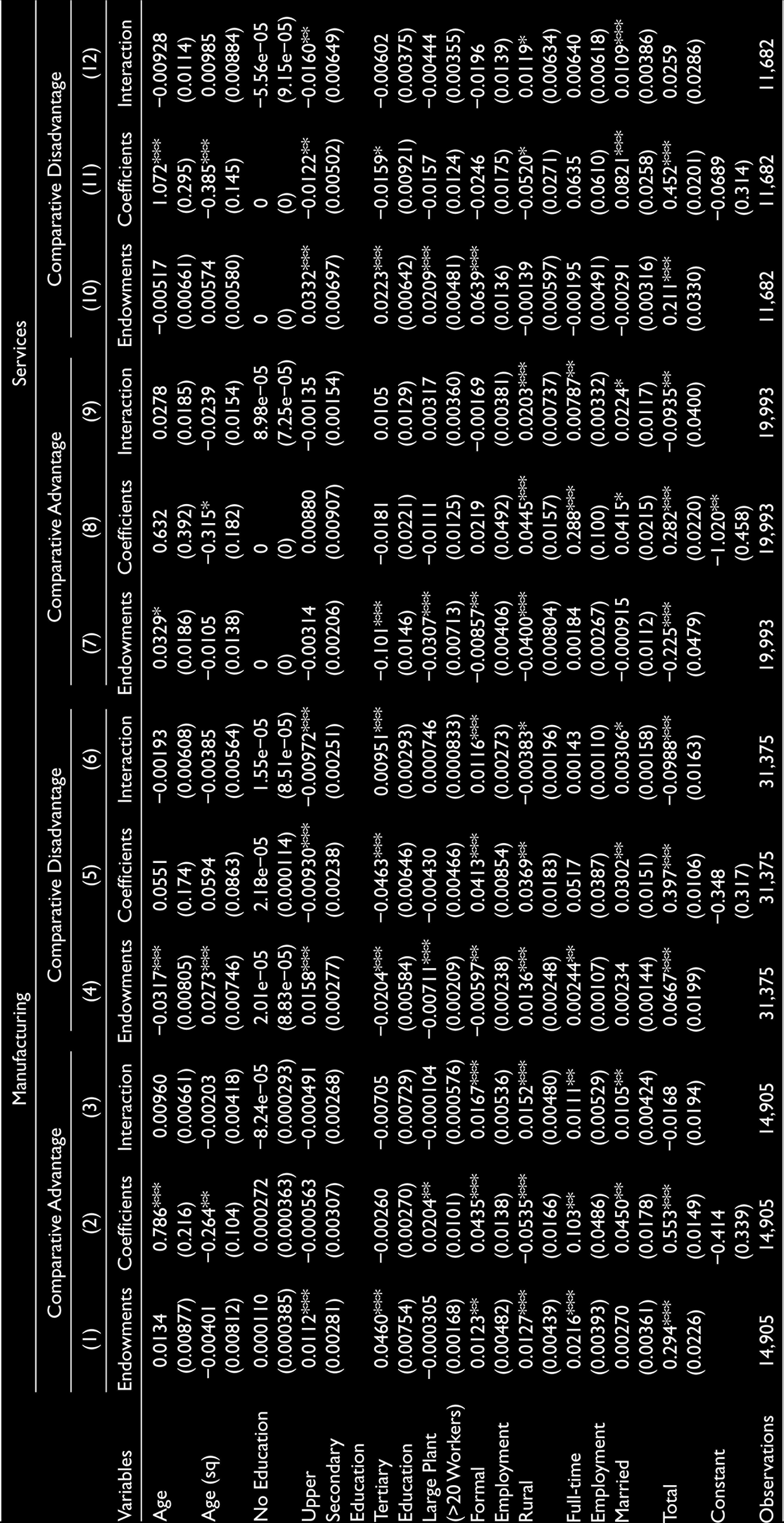
Appendix

Table A4.

Oaxaca–Blinder Decomposition, Wages.

Variables	Manufacturing						Services
	Comparative Advantage			Comparative Disadvantage			Comparative Advantage			Comparative Disadvantage
	(1)	(2)	(3)	(4)	(5)	(6)	(7)	(8)	(9)	(10)	(11)	(12)
	Endowments	Coefficients	Interaction	Endowments	Coefficients	Interaction	Endowments	Coefficients	Interaction	Endowments	Coefficients	Interaction
Age	0.0134	0.786***	0.00960	−0.0317***	0.0551	−0.00193	0.0329*	0.632	0.0278	−0.00517	1.072***	−0.00928
	(0.00877)	(0.216)	(0.00661)	(0.00805)	(0.174)	(0.00608)	(0.0186)	(0.392)	(0.0185)	(0.00661)	(0.295)	(0.0114)
Age (sq)	−0.00401	−0.264**	−0.00203	0.0273***	0.0594	−0.00385	−0.0105	−0.315*	−0.0239	0.00574	−0.385***	0.00985
	(0.00812)	(0.104)	(0.00418)	(0.00746)	(0.0863)	(0.00564)	(0.0138)	(0.182)	(0.0154)	(0.00580)	(0.145)	(0.00884)
No Education	0.000110	0.000272	−8.24e−05	2.01e−05	2.18e−05	1.55e−05	0	0	8.98e−05	0	0	−5.56e−05
	(0.000385)	(0.000363)	(0.000293)	(8.83e−05)	(0.000114)	(8.51e−05)	(0)	(0)	(7.25e−05)	(0)	(0)	(9.15e−05)
Upper Secondary Education	0.0112***	−0.000563	−0.000491	0.0158***	−0.00930***	−0.00972***	−0.00314	0.00880	−0.00135	0.0332***	−0.0122**	−0.0160**
Upper Secondary Education	(0.00281)	(0.00307)	(0.00268)	(0.00277)	(0.00238)	(0.00251)	(0.00206)	(0.00907)	(0.00154)	(0.00697)	(0.00502)	(0.00649)
Tertiary Education	0.0460***	−0.00260	−0.00705	−0.0204***	−0.0463***	0.00951***	−0.101***	−0.0181	0.0105	0.0223***	−0.0159*	−0.00602
Tertiary Education	(0.00754)	(0.00270)	(0.00729)	(0.00584)	(0.00646)	(0.00293)	(0.0146)	(0.0221)	(0.0129)	(0.00642)	(0.00921)	(0.00375)
Large Plant (>20 Workers)	−0.000305	0.0204**	−0.000104	−0.00711***	−0.00430	0.000746	−0.0307***	−0.0111	0.00317	0.0209***	−0.0157	−0.00444
Large Plant (>20 Workers)	(0.00168)	(0.0101)	(0.000576)	(0.00209)	(0.00466)	(0.000833)	(0.00713)	(0.0125)	(0.00360)	(0.00481)	(0.0124)	(0.00355)
Formal Employment	0.0123**	0.0435***	0.0167***	−0.00597**	0.0413***	0.0116***	−0.00857**	0.0219	−0.00169	0.0639***	−0.0246	−0.0196
Formal Employment	(0.00482)	(0.0138)	(0.00536)	(0.00238)	(0.00854)	(0.00273)	(0.00406)	(0.0492)	(0.00381)	(0.0136)	(0.0175)	(0.0139)
Rural	0.0127***	−0.0535***	0.0152***	0.0136***	0.0369**	−0.00383*	−0.0400***	0.0445***	0.0203***	−0.00139	−0.0520*	0.0119*
	(0.00439)	(0.0166)	(0.00480)	(0.00248)	(0.0183)	(0.00196)	(0.00804)	(0.0157)	(0.00737)	(0.00597)	(0.0271)	(0.00634)
Full-time Employment	0.0216***	0.103**	0.0111**	0.00244**	0.0517	0.00143	0.00184	0.288***	0.00787**	−0.00195	0.0635	0.00640
Full-time Employment	(0.00393)	(0.0486)	(0.00529)	(0.00107)	(0.0387)	(0.00110)	(0.00267)	(0.100)	(0.00332)	(0.00491)	(0.0610)	(0.00618)
Married	0.00270	0.0450**	0.0105**	0.00234	0.0302**	0.00306*	−0.000915	0.0415*	0.0224*	−0.00291	0.0821***	0.0109***
	(0.00361)	(0.0178)	(0.00424)	(0.00144)	(0.0151)	(0.00158)	(0.0112)	(0.0215)	(0.0117)	(0.00316)	(0.0258)	(0.00386)
Total	0.294***	0.553***	−0.0168	0.0667***	0.397***	−0.0988***	−0.225***	0.282***	−0.0935**	0.211***	0.452***	0.0259
	(0.0226)	(0.0149)	(0.0194)	(0.0199)	(0.0106)	(0.0163)	(0.0479)	(0.0220)	(0.0400)	(0.0330)	(0.0201)	(0.0286)
Constant		−0.414			−0.348			−1.020**			−0.0689
		(0.339)			(0.317)			(0.458)			(0.314)
Observations	14,905	14,905	14,905	31,375	31,375	31,375	19,993	19,993	19,993	11,682	11,682	11,682

Source: Authors’ own regression results.

Notes: Fixed effects include industry, year, occupations, state, household size, and land ownership.

Robust standard errors in parentheses ***P < .01, **P < .05, *P < .1.

Notes

References

Becker

G. S.

(1971). The economics of discrimination. University of Chicago Press.

Black

S. E.

, & Brainerd

(2004). Importing equality? The impact of globalization on gender discrimination. Industrial and Labor Relations Review, 57(4), 540. https://doi.org/10.2307/4126682

Blau

F. D.

, & Kahn

L. M.

(2017). The gender wage gap: Extent, trends, and explanations. Journal of Economic Literature, 55(3), 789–865.

Chamarbagwala

(2006). Economic liberalization and wage inequality in India. World Development, 34(12), 1997–2015.

Duraisamy

, & Duraisamy

(2016). Gender wage gap across the wage distribution in different segments of the Indian labour market, 1983–2012: Exploring the glass ceiling or sticky floor phenomenon. Applied Economics, 48(43), 4098–4111. https://doi.org/10.1080/00036846.2016.1150955

Dutta

P. V.

, & Reilly

(2008). The gender pay gap in an era of economic change: Evidence for India, 1983 to 2004. The Indian Journal of Labour Economics, 51(3), 341–366.

International Labour Organization (2018). India wage report: Wage policies for decent work and inclusive growth. Author.

Juhn

, Ujhelyi

, & Villegas-Sanchez

(2014). Men, women, and machines: How trade impacts gender inequality. Journal of Development Economics. https://doi.org/10.1016/j.jdeveco.2013.09.009

Kis-Katos

, Pieters

, & Sparrow

(2018). Globalization and social change: Gender-specific effects of trade liberalization in Indonesia. IMF Economic Review, 66(4), 763–793. https://doi.org/10.1057/s41308-018-0065-5

10.

Kuruvilla

, & Ranganathan

(2010). Globalisation and outsourcing: Confronting new human resource challenges in India’s business process outsourcing industry. Industrial Relations Journal, 41(2), 136–153.

11.

Laursen

(2015). Revealed comparative advantage and the alternatives as measures of international specialization. Eurasian Business Review, 5(1), 99–115. https://doi.org/10.1007/s40821-015-0017-1

12.

Melitz

M. J.

(2003). The impact of trade on intra-industry reallocations and aggregate industry productivity. Econometrica. https://doi.org/10.1111/1468-0262.00467

13.

Menon

, & van der Meulen Rodgers

(2009). International trade and the gender wage gap: New evidence from India’s manufacturing sector. World Development, 37(5), 965–981. https://doi.org/10.1016/j.worlddev.2008.09.009

14.

Nataraj

(2011). The impact of trade liberalization on productivity: Evidence from India’s formal and informal manufacturing sectors. Journal of International Economics (Elsevier BV), 85(2), 292–301. https://doi.org/10.1016/j.jinteco.2011.07.003

15.

Nordås

H. K.

(2003). The impact of trade liberalization on women’s job opportunities and earnings in developing countries. World Trade Review, 2(02), 221–231. https://doi.org/10.1017/s1474745603001381

16.

Oaxaca

(1973). Male-female wage differentials in urban labor markets. International Economic Review, 14(3), 693. https://doi.org/10.2307/2525981

17.

Timmer

M. P.

, Dietzenbacher

, Los

, Stehrer

, & de Vries

G. J.

(2015). An illustrated user guide to the world input-output database: The case of global automotive production. Review of International Economics, 23(3), 575–605. https://doi.org/10.1111/roie.12178

18.

Weichselbaumer

, & Winter-Ebmer

(2005). A meta-analysis of the international gender wage gap. Journal of Economic Surveys, 19(3), 479–511. https://doi.org/10.1111/j.0950-0804.2005.00256.x

19.

World Bank (2012). World development report 2012: Gender equality and development. Author.

20.

Yeats

A. J.

(1985). On the appropriate interpretation of the revealed comparative advantage index: Implications of a methodology based on industry sector analysis. Weltwirtschaftliches Archive, 121(1), 61–73.

Services Trade: The Great Gender Equaliser?

Abstract

Keywords

Introduction

Relations to Previous Research

Data

Revealed Symmetrical Comparative Advantage

Descriptive Statistics

Explaining the Gender Wage Gap

Concluding Remarks

Footnotes

Declaration of Conflicting Interests

Funding

Appendix

Notes

References