Sage Journals: Discover world-class research

Abstract

Applied researchers often encounter situations where certain item response categories receive very few endorsements, resulting in sparse data. Collapsing categories may mitigate sparsity by increasing cell counts, yet the methodological consequences of this practice remain insufficiently explored. The current study examined the effects of response collapsing in Likert-type scale data through a simulation study under the confirmatory factor analysis model. Sparse response categories were collapsed to determine the impact on fit indices (i.e., chi-square, comparative fit index [CFI], Tucker–Lewis index [TLI], root mean square error of approximation [RMSEA], and standardized root mean square residual [SRMR]). Findings indicate that category collapsing has a significant impact when sparsity is severe, leading to reduced model rejections in both correctly specified and misspecified models. In addition, different fit indices exhibited varying sensitivities to data collapsing. Specifically, RMSEA was recommended for the correctly identified model, and TLI with a cut-off value of .95 was recommended for the misspecified models. The empirical analysis was aligned with the simulation results. These results provide valuable insights for researchers confronted with sparse data in applied measurement contexts.

Keywords

sparse responses collapsing confirmatory factor analysis model fit

Introduction

In survey research, the Likert-type scale is among the most commonly employed item formats for data collection (Eichhorn, 2022). A Likert-type scale “has multiple categories from which respondents choose to indicate their opinions, attitudes, or feelings about a particular issue” (Nemoto & Beglar, 2014). Compared to open-ended questions, researchers can easily generate numerical quantitative results with data from Likert-type scale questions (e.g., calculating mean and standard deviation) to efficiently facilitate data analysis. The standardized format of a Likert-type scale for all survey items improves the reliability and validity by reducing ambiguity in response interpretations (Joshi et al., 2015).

One key advantage of Likert-type scales is their flexibility in design, as researchers can determine the number of response options and the labels used to describe them depending on the research purpose. However, it is important to recognize that individual Likert-type scale items yield ordinal data, where response options follow a ranked order but do not necessarily maintain equal intervals between categories (Sullivan & Artino, 2013). Research on various design elements of Likert-type scales—including scale length, response labels, and the number of response categories—has been extensively studied (e.g., Aybek & Toraman, 2022; Horan et al., 2003; Kankaraš & Capecchi, 2024; Lee & Paek, 2014). Among these factors, the number of response categories has received particular attention due to its substantial impact on measurement reliability and validity (Lozano et al., 2008).

Optimal Number of Response Categories

The optimal number of response categories for achieving high measurement quality remains a topic of debate in prior literature. In general, researchers argue that increasing the number of response options enhances psychometric properties up to a certain point. For example, Preston and Colman (2000) found that scales with five or more response options yield higher internal consistency and test–retest reliability compared to scales with fewer alternatives. Similarly, Lozano et al. (2008) demonstrated that while reliability and validity estimates improve with additional response options, these improvements tend to plateau at around seven categories based on existing simulation studies. This pattern is consistent with Matell and Jacoby (1971), who showed that reliability and validity increased sharply as the number of categories rose from two to about seven. Likewise, Oaster (1989) reported that increasing the number of response options from three to seven improved the stability of the results. On the contrary, other studies concluded that five categories are preferable to seven or eleven categories based on multitrait-multimethod analyses (e.g., Revilla et al., 2014).

While prior studies focused on basic psychometric analysis, recent studies have extended the investigation of the number of response categories into the confirmatory factor analysis (CFA) framework. CFA is a multivariate statistical method that tests whether data fits a pre-specified measurement model linking observed variables to their underlying latent constructs, offering advantages over traditional psychometric analyses by rigorously assessing model fit and complex inter-item relationships (Brown, 2015). Within this framework, Li (2016) reported that increasing the number of categories from four to ten can enhance the accuracy of factor loadings and inter-factor correlation estimates. In line with these findings, Maydeu-Olivares and colleagues (2017) recommended including at least five response alternatives in measurement instruments, highlighting concerns regarding model fit and the precision of parameter estimates. DiStefano and colleagues (2018) identified that the model fit indices of five response categories are better compared to two response categories while other parameters are consistent.

Model Estimation and Item Distribution

Despite inconsistent findings in previous studies, choosing the appropriate number of response options remains a significant decision in scale design and/or psychometric analysis, as it directly impacts the selection of the appropriate model estimation method in CFA (DiStefano & Morgan, 2014). Although Likert-type scale item responses represent ordered categories without equal interval spacing, researchers often treat them as approximately continuous by applying maximum likelihood (ML) estimation (Rhemtulla et al., 2012). This practice is problematic because the assumption of multivariate normality is frequently violated (Finney & DiStefano, 2013), particularly when fewer than five response categories are used (Rhemtulla et al., 2012). Although alternative ML-based estimators, such as Maximum Likelihood with Mean and Variance adjustment (MLMV), can help mitigate non-normality, they do not fully account for the ordinal nature of Likert-type scale data, as these methods treat responses as continuous and assume underlying interval-level measurement (Finney & DiStefano, 2013).

Employing estimation methods unsuitable for the data type can lead to biased parameter estimates and incorrect inferences (Rhemtulla et al., 2012) on CFA. To address this issue, alternative robust estimation methods, such as Unweighted Least Squares Mean and Variance Adjusted (ULSMV) and Weighted Least Squares Mean and Variance Adjusted (WLSMV), have been recommended (Finney & DiStefano, 2006) to appropriately account for the ordinal nature using polychoric correlations instead of Pearson correlations (Li, 2016).

Handling Sparse Data

One contributing factor to non-normality in Likert-type scale responses is sparse data, where certain response categories attract very few endorsements (DiStefano et al., 2021). Sparse data can result in excessively skewed distributions and increased kurtosis, further complicating model estimation processes. Sparse data are frequently observed in practice. For instance, social desirability may lead respondents to select extreme endpoints of an item (Liu et al., 2017), thereby reducing the frequency of intermediate responses. Such patterns have been observed in scales measuring academic dishonesty and alcohol consumption (e.g., Davis et al., 2010; Winrow et al., 2015), as well as in clinical and screening instruments assessing behavioral or psychiatric symptoms, where certain severity categories are rarely endorsed (e.g., Bowden et al., 2007; Wang et al., 2021). Overall, it is essential to select appropriate estimation methods that can properly account for sparse data, given its impact on model fit and parameter estimation (Li, 2016; Liang & Yang, 2014).

Sparseness levels can range from zero (Savalei, 2011) to low frequencies in certain categories (DiStefano et al., 2021; Rhemtulla et al., 2012). For low frequencies, the definition of “sparseness” in categorical data varies across researchers. For instance, Rutkowski et al. (2019) recommended collapsing categories when a cell contained fewer than 10 responses, whereas DiStefano et al. (2021) identified sparsity based on low percentages, typically 2% or 4% of the total response. Various methods have been proposed to address sparse data. Researchers could manually add a threshold to the category (categories) without any response (Savalei, 2011; Yang & Weng, 2024). However, this strategy is generally recommended for binary data rather than for items with more than two response categories. Another common approach is to collapse certain subcategories for all items to form a new category with greater frequencies (e.g., Zhao et al., 2023).

Researchers have explored the effect of collapsing responses, an alternative perspective examining the number of response categories. In a study of the Rosenberg Self-Esteem scale, Colvin and Gorgun (2020) found that models based on collapsed responses demonstrated better model fit indices than those using the original data. They suggested that while the scale should be administered in its original format, collapsing responses prior to data analysis may be beneficial. An earlier simulation study also confirmed the advantages of collapsing categories in CFA (Grimbeek et al., 2005). The results showed that collapsing responses from five categories to two categories illustrated a better fit (e.g., root mean square error of approximation [RMSEA], standardized root mean square residual [SRMR], chi-square tests).

Most prior studies collapsed all responses to reduce the number of categories. However, in practice, items within a scale often exhibit varying response distributions, and only a subset of items may exhibit sparse response patterns. Collapsing all items can lead to the loss of meaningful information, particularly for non-sparse items, and may introduce overgeneralization. An alternative approach is to collapse response categories only for items with sparse responses while preserving the original structure for non-sparse items (i.e., infrequent collapsing).

A recent study using measurement invariance testing, a follow-up test based on CFA result, suggested a meaningful impact on the model fit by employing infrequent collapsing, where only sparse categories of corresponding items are collapsed (Rutkowski et al., 2019). This study introduced new possibilities for applying collapsing strategies in CFA. In addition, infrequent collapsing allows for a more nuanced approach that retains the variability and interpretability of non-sparse items. DiStefano and colleagues (2021) examined infrequent collapsing in the framework of CFA and found that collapsing categories only for items with sparse responses was advantageous compared to analyzing the original data. When sparse categories were collapsed, results showed higher model convergence rates, more accurate parameter estimates, smaller standard errors, and chi-square testing rejection rates close to .05 under manipulated conditions (e.g., sample size, number of items with sparse data).

However, the authors did not include certain modeling conditions that warrant additional investigation. For instance, only correctly specified models were considered to study Type I error rates; however, model misspecification is a common practical condition in CFA models (Chen et al., 2008; DiStefano et al., 2018; Shi et al., 2019). Furthermore, more practical modeling conditions (e.g., different response categories & high or low factor loadings) remain underexplored. Finally, the performance of additional fit indices on top of the chi-square results has not been examined.

The Present Study

Therefore, the current study was conducted to fill the above research gaps. The following model fit indices were considered the main output in the current study. The chi-square fit index is an exact fit test, measuring the discrepancy between the observed data and the model-implied covariance matrix. Conceptually, observed covariances represent the actual relationships between items in the sample data, while predicted covariances are the expected relationships estimated by the model. Chi-square tests are sensitive to sample size. In large samples, even minor discrepancies between the observed and predicted covariances can lead to a significant chi-square result, which may incorrectly indicate model misfit (DiStefano, 2016). On the contrary, it is not realistic to expect an exact fit in practice due to the concern of measurement error and model complexity (Goretzko et al., 2024). Therefore, alternative fit indices were evaluated.

RMSEA is an absolute fit index that measures the misfit level of the hypothesized model by considering sample size and model complexity. As a “badness-of-fit” index, RMSEA reflects the degree of model misfit, with higher values indicating poorer fit (Kline, 2011; MacCallum et al., 1996). SRMR is another absolute fit index measuring the average standardized residuals between observed and predicted correlation matrices (Kline, 2011). It is also considered a badness-of-fit index, ranging from 0 to 1, with lower values indicating better fit. The comparative fit index (CFI) and Tucker–Lewis index (TLI) are incremental fit indices that measure the relative improvement in the fit of a hypothesized model compared to a baseline model, which assumes no relationships among the observed variables (Xia & Yang, 2019). CFI and TLI typically range from 0 to 1, with higher values indicating better model fit.

This study aims to provide a comprehensive understanding of various fit indices in the context of sparse data and infrequent collapsing. Specifically, this study investigates how correctly specified and misspecified models perform across different model fit indices while considering other modeling factors (e.g., degree of factor loadings, degree of item sparse levels, and sample size). Specifically, the study examines the model rejection rates and the stability of chi-square, CFI, TLI, RMSEA, and SRMR across correctly specified and misspecified models. This study seeks to provide practical guidance for researchers in selecting and interpreting fit indices more effectively when sparse data and model misspecification are present.

Methods

A Monte Carlo simulation study was conducted to examine the effect of collapsing item responses with sparse data. While many studies advocated for five or more response categories to enhance psychometric properties, the selection of a four-category scale was intentional. This choice aligns with findings that scales with four to seven response categories offer an optimal balance between psychometric properties and respondent burden (Lozano et al., 2008). As five response categories were generally recommended as the minimum for treating data as continuous (Rhemtulla et al., 2012), we selected four categories to ensure the use of a robust estimation method appropriate for ordinal data. Consequently, we employed the WLSMV estimator, which is specifically designed for ordinal data and does not assume normality. Data were generated in Mplus 8.11 (Muthén & Muthén, 2017). A three-factor CFA population model was specified: each factor was measured by five items, yielding 15 items in total. The factor correlations were fixed at .40.

Model Specification

Model specifications were established to assess the adequacy of model identification, wherein a correctly specified model should be retained, and a misspecified model should be rejected, based on statistical fit criteria (Goretzko et al., 2024; Shi & Maydeu-Olivares, 2020). Three conditions were estimated: (a) a correctly specified model with all items loading on the factors matching the population model, (b) Misspecification 1 with one item loading on a different factor (i.e., mild misspecification), and (c) misspecification with two factors collapsed (i.e., severe misspecification). These conditions are displayed in Figure 1.

Figure 1.

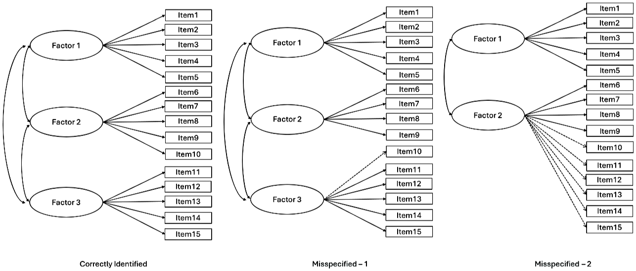
Model Specification.

Factor Loadings

Factor loadings influence the performance of model fit, with higher factor loadings generally leading to better model fit. All factor loadings set at .80 represented a high loading condition, and factor loadings set at .50 represented a moderate loading condition (DiStefano et al., 2018).

Sample Size

Sample size is a common factor to vary in simulation studies of CFA (Wolf et al., 2013). Two sample sizes were considered: N = 250 and N = 500, corresponding to sample size to number of items ratios of 17:1 and 33:1.

Sparse Data

The term “sparse” is somewhat subjective, as its definition can vary across studies. In this study, both the number of items and the degree of sparsity within each item were manipulated to represent different levels of sparsity, following the guidelines of prior research (DiStefano et al., 2021). Per factor, we considered the following three conditions: one item with sparse data, two items with sparse data, and four items with sparse data. Among these items with sparse data, we set up percentages of responses per category using different thresholds. Different distributions were considered, indicating the degree of sparse responses of each item. In one category with sparse responses, the initial percentages of 30%, 40%, 28%, and 2% were consolidated into 30%, 40%, and 30%. For two categories exhibiting sparse responses, the original distribution of 46%, 50%, 2%, and 2% was merged into 46% and 54% to eliminate sparseness. When three categories had sparse responses, the initial percentages of 94%, 2%, 2%, and 2% were combined into 94% and 6%. After sparse data were generated, sparse responses were recoded to generate collapsed data.

In sum, the simulation design included the following manipulated conditions: model specification (three levels), factor loadings (two levels), sample size (two levels), number of items with sparse responses (three levels), item response distributions (three levels), and data collapsing strategies (two levels), resulting in a total of 216 unique conditions. For each condition, 1,000 replications were conducted.

Data Analysis

First, model convergence rates were computed to show the percentages of completed replications for each simulation condition; percentages above .90 are generally considered acceptable (Gagné & Hancock, 2006; Moshagen & Musch, 2014). We then used multiple model fit indices to evaluate the performance of CFA models across simulation conditions: chi-square, RMSEA, CFI, TLI and SRMR. For chi-square statistics, when the model is correctly specified, researchers intend to control the Type I error rate (i.e., inappropriate rejection) at the nominal alpha level (i.e., .05). Conversely, when the model is misspecified, researchers expect it to be correctly rejected, reflecting statistical power. Statistical power is conventionally expected to reach the established threshold of .80 (Cohen, 1988).

For other fit indices, we referred to the following criteria: CFI ≥ .90, TLI ≥ .90, SRMR ≤ .10, and RMSEA ≤ .08 were considered to indicate adequate model fit; CFI ≥ .95, TLI ≥ .95, SRMR ≤ .08, and RMSEA ≤ .05 were considered to indicate good model fit (Hu & Bentler, 1999). In each replication of one condition, a model could be rejected or retained based on the comparison between the estimate and the cut-off value. Accumulating the model fit results across 1000 repetitions, model rejection rates were calculated based on the defined cut-off value for each condition. It was expected to retain the model when the model is misspecified at the level of .05, while we expect to reject the model when the model is correctly identified (80% or higher) in the long term. In each replication, model fit values were saved and then summarized across replications to indicate the fit stability using the mean and standard deviation.

Empirical Illustration

Scale

The revised version of the Ethics Position Questionnaire (EPQ-5; O’Boyle & Forsyth, 2021) is a shortened 10-item form of Forsyth’s (1980) original 20-item EPQ. Respondents rated their agreement with each statement on a five-point Likert-type scale: strongly agree, somewhat agree, neutral, somewhat disagree, and strongly disagree (5 to 1). The EPQ-5 consists of two subscales—Idealism (Items 1–5) and Relativism (Items 6–10; Table 1). Idealism measures concern for minimizing harm and maximizing benefits, while Relativism represents a focus on ethical flexibility and rejection of absolute moral principles. Higher Idealism scores indicate stricter ethical judgments, and higher Relativism scores indicate less adherence to universal moral rules. O’Boyle and Forsyth (2021) confirmed the two-factor structure, established measurement invariance across gender groups, and showed evidence of predictive and convergent validity through associations with related constructs.

Table 1.

Frequency Table of the Ethics Position Scale Items.

Items	Content	Response categories
Items	Content	5	4	3	2	1
1	A person should make certain that their actions never intentionally harm another even to a small degree.	57.6	25.7	10.9	3.1	2.7
2	The existence of potential harm to others is always wrong, irrespective of the benefits to be gained.	49.6	25.5	14.4	7.0	3.5
3	One should never psychologically or physically harm another person.	71.8	15.6	6.6	3.5	2.5
4	One should not perform an action that might in any way threaten the dignity and welfare of another individual.	68.7	18.7	7.2	3.1	2.3
5	If an action could harm an innocent other, then it should not be done.	68.7	18.9	7.8	2.5	2.1
6	What is ethical varies from one situation and society to another.	31.9	36.8	17.9	8.8	4.7
7	Moral standards should be seen as being individualistic; what one person considers to be moral may be judged to be immoral by another person.	21.6	32.1	25.5	15.6	5.3
8	Questions of what is ethical for everyone can never be resolved since what is moral or immoral is up to the individual.	14.6	30.5	25.5	22.4	7.0
9	Moral standards are simply personal rules that indicate how a person should behave and are not to be applied in making judgments of others.	17.1	26.3	24.5	23.7	8.4
10	Ethical considerations in interpersonal relations are so complex that individuals should be allowed to formulate their own individual codes.	15.2	28.4	30.4	19.1	7.0

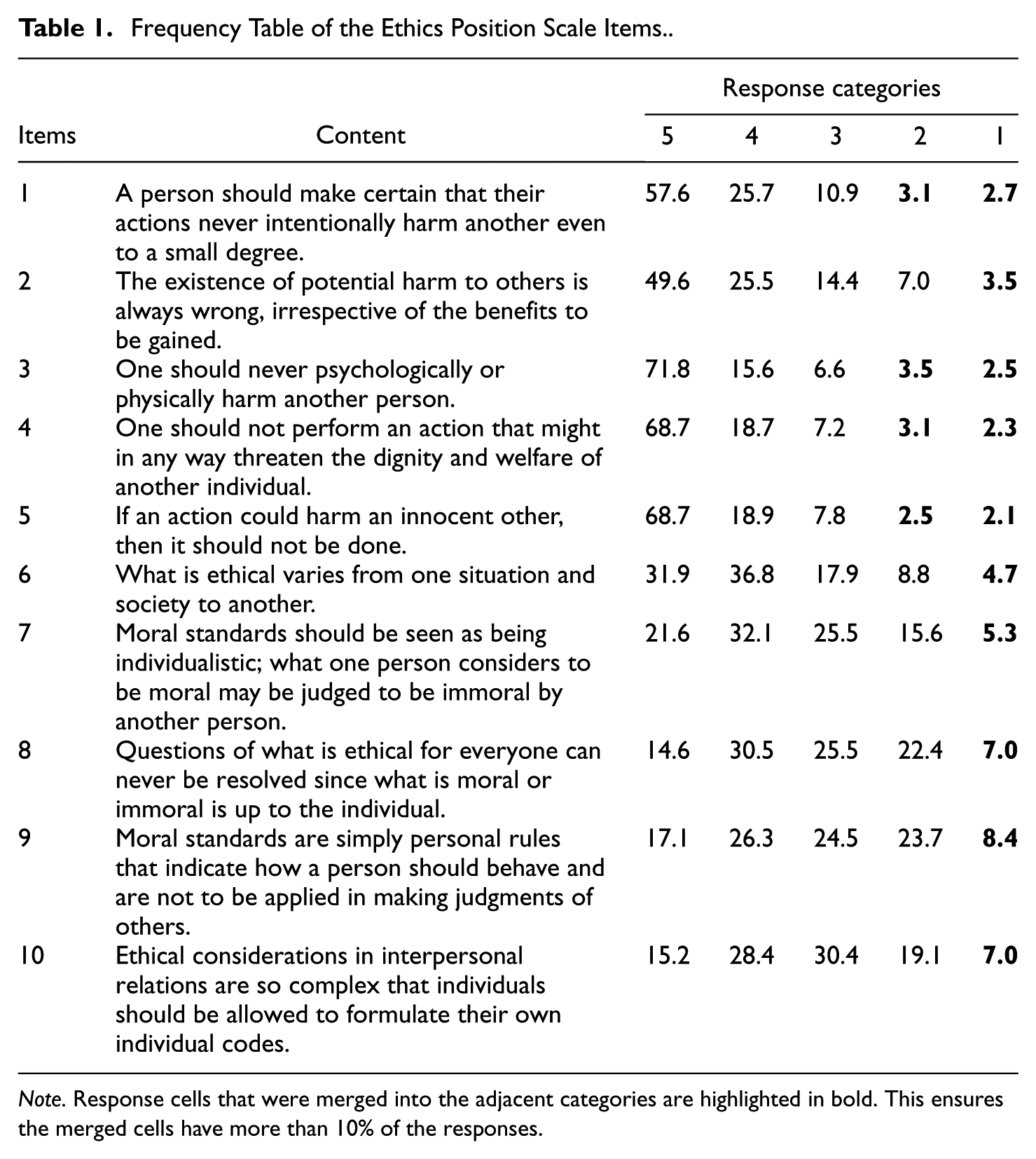
Note. Response cells that were merged into the adjacent categories are highlighted in bold. This ensures the merged cells have more than 10% of the responses.

Data Collection/Sample

Participants included students from diverse program areas and grade levels at an R1 university. Recruitment occurred through instructors of selected courses and via school email invitations or QR codes in the academic year of 2023 to 2024. The EPQ-5 was included as part of a larger survey study. A total of 514 students completed the survey, with 77.4% (n = 398) being undergraduates and 22.6% (n = 116) graduate students. Most participants were aged 18–24 (n = 431, 83.9%). The sample comprised 310 females (60.3%), 194 males (37.7%), and 10 respondents identifying as another gender (1.9%). In terms of race/ethnicity, 358 participants (69.6%) identified as White (non-Hispanic), 54 as African American (10.5%), 42 as Asian (8.2%), 32 as Hispanic (6.2%), and 28 as other races (5.4%).

Data manipulation

There was no missing data. Most sparse cells (<10%) occurred in Response Options 1 and 2, indicating the small chance of selecting disagree-related categories. We merged these cells with the next adjacent category/categories to mitigate sparse levels. The goal was to obtain a collapsed data file with all cells that were higher than 10%. For instance, Categories 1 and 2 were merged into Category 3 in Item 1. Consequently, two data sets were included—one before and one after collapsing—for comparative analysis following the same evaluation criteria described in the simulation phase. Finally, given that the theoretical framework of the scale was well-established in prior literature (O’Boyle & Forsyth, 2021), the two-factor model was treated as the correctly specified model. A minor misspecification was also introduced by loading Item 6 from Relativism to Idealism.

Results

Convergence Rates

Overall, convergence rates were high across the set of cells in the study design; low convergence rates were observed under certain conditions (e.g., sample size of 250, low loadings, and four items with sparse responses in three categories), indicating that results in these scenarios should be interpreted cautiously (Table 2). Notably, sparsity persisted even after collapsing when four items contained sparse responses. Collapsing sparse ordinal data significantly improved convergence rates in these conditions. For example, when the sample size was 250, factor loadings were moderate, and three response categories contained sparse data across four items, the convergence rate increased from .308 to .992 when the data were collapsed. Collapsing sparse data also increased convergence rates when the models were misspecified. In other words, collapsing sparse data may raise the likelihood of identifying an incorrect model.

Table 2.

Convergence Rates.

Model specification				One item			Two items			Four items
Model specification				1Cat	2Cat	3Cat	1Cat	2Cat	3Cat	1Cat	2Cat	3Cat
Correctly identified (N = 6, 6.94%)	High loadings	N = 250	Sparse	0.977	0.963	0.922	0.964	0.929	0.845	0.924	0.855	0.750
		N = 250	Collapse	1.000	1.000	0.975	1.000	1.000	0.946	1.000	1.000	0.970
		N = 500	Sparse	1.000	1.000	1.000	1.000	1.000	0.999	0.999	0.999	0.998
		N = 500	Collapse	1.000	1.000	1.000	1.000	1.000	0.999	1.000	1.000	1.000
	Low loadings	N = 250	Sparse	0.985	0.960	0.922	0.962	0.921	0.637	0.920	0.843	0.308
		N = 250	Collapse	1.000	1.000	1.000	1.000	1.000	1.000	1.000	1.000	0.992
		N = 500	Sparse	1.000	1.000	0.997	1.000	1.000	0.979	1.000	1.000	0.701
		N = 500	Collapse	1.000	1.000	1.000	1.000	1.000	1.000	1.000	1.000	1.000
M1 (N = 6, 8.33%)	High loadings	N = 250	Sparse	0.977	0.963	0.922	0.964	0.929	0.845	0.924	0.855	0.735
		N = 250	Collapse	1.000	1.000	0.975	1.000	1.000	0.946	1.000	1.000	0.970
		N = 500	Sparse	1.000	1.000	1.000	1.000	1.000	0.999	0.999	0.999	0.997
		N = 500	Collapse	1.000	1.000	1.000	1.000	1.000	0.999	1.000	1.000	1.000
	Low loadings	N = 250	Sparse	0.985	0.960	0.895	0.962	0.921	0.597	0.920	0.843	0.324
		N = 250	Collapse	1.000	1.000	1.000	1.000	1.000	1.000	1.000	1.000	0.977
		N = 500	Sparse	1.000	1.000	0.996	1.000	1.000	0.957	1.000	1.000	0.615
		N = 500	Collapse	1.000	1.000	1.000	1.000	1.000	1.000	1.000	1.000	0.996
M2 (N = 6, 8.33%)	High loadings	N = 250	Sparse	0.977	0.963	0.922	0.964	0.929	0.845	0.924	0.855	0.763
		N = 250	Collapse	1.000	1.000	0.975	1.000	1.000	0.946	1.000	1.000	0.970
		N = 500	Sparse	1.000	1.000	1.000	1.000	1.000	0.999	0.999	0.999	0.998
		N = 500	Collapse	1.000	1.000	1.000	1.000	1.000	0.999	1.000	1.000	1.000
	Low loadings	N = 250	Sparse	0.985	0.960	0.937	0.962	0.921	0.761	0.920	0.843	0.486
		N = 250	Collapse	1.000	1.000	1.000	1.000	1.000	1.000	1.000	1.000	0.996
		N = 500	Sparse	1.000	1.000	0.999	1.000	1.000	0.990	1.000	1.000	0.823
		N = 500	Collapse	1.000	1.000	1.000	1.000	1.000	1.000	1.000	1.000	1.000

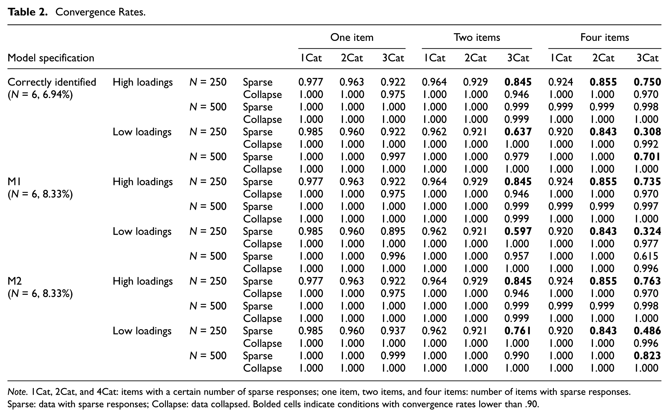
Note. 1Cat, 2Cat, and 4Cat: items with a certain number of sparse responses; one item, two items, and four items: number of items with sparse responses. Sparse: data with sparse responses; Collapse: data collapsed. Bolded cells indicate conditions with convergence rates lower than .90.

Model Rejection Rates

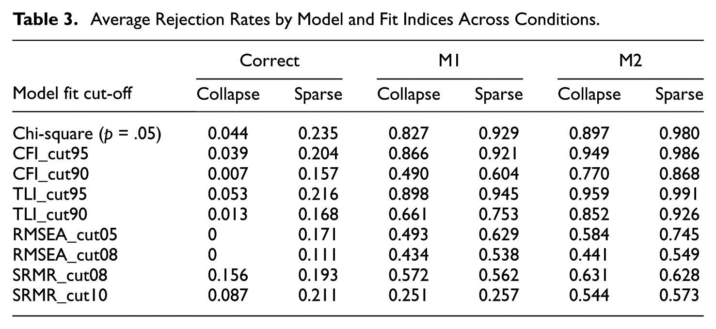
In the following sections, we summarized results for the fit indices of interest. To describe the patterns, we calculated the average model rejection rates by fit indices for each model (Table 3). Overall, average rejection rates were below .05 under the correctly specified model for collapsed responses, indicating that Type I error was generally controlled after collapsing. As expected, average rejection rates increased sharply under M1 (mild misspecification) and M2 (severe misspecification), with the highest rates observed for M2, especially with sparse responses. Sparse responses consistently yielded higher rejection rates than collapsed responses. Among the indices, CFI (.95), TLI (.95), and chi-square showed the strong ability to detect misspecification, while RMSEA (.05/.08) and SRMR (.08/.10) were more conservative, with lower rejection rates.

Table 3.

Average Rejection Rates by Model and Fit Indices Across Conditions.

Model fit cut-off	Correct		M1		M2
Model fit cut-off	Collapse	Sparse	Collapse	Sparse	Collapse	Sparse
Chi-square (p = .05)	0.044	0.235	0.827	0.929	0.897	0.980
CFI_cut95	0.039	0.204	0.866	0.921	0.949	0.986
CFI_cut90	0.007	0.157	0.490	0.604	0.770	0.868
TLI_cut95	0.053	0.216	0.898	0.945	0.959	0.991
TLI_cut90	0.013	0.168	0.661	0.753	0.852	0.926
RMSEA_cut05	0	0.171	0.493	0.629	0.584	0.745
RMSEA_cut08	0	0.111	0.434	0.538	0.441	0.549
SRMR_cut08	0.156	0.193	0.572	0.562	0.631	0.628
SRMR_cut10	0.087	0.211	0.251	0.257	0.544	0.573

Then, we presented line graphs of model rejection rates under simulation conditions. We organized the results by the model specification type (Figures 2 –4). In each figure, 72 model rejection rates were plotted (factor loadings * 2, sample size * 2, number of items with sparse responses * 3, item response distributions * 3, and data collapsing strategies * 2). The number of inflated model rejection rates was reported under each subfigure. Finally, the stability of fit indices was estimated using the boxplots. Full results across conditions and fit distribution are available in the Supplemental Materials.

Figure 2.

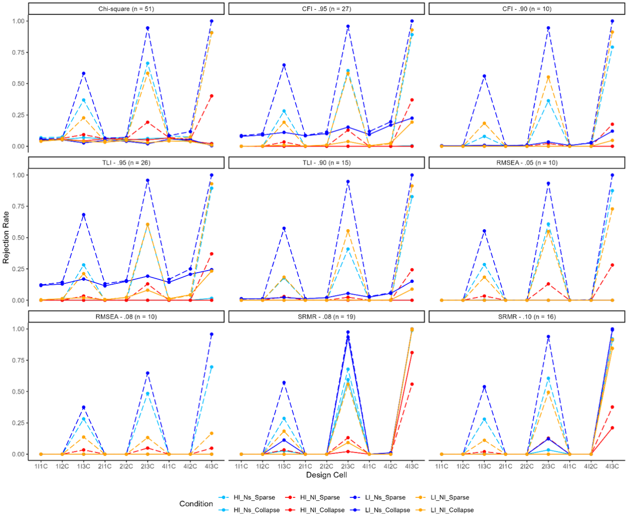
Model Rejection Rates Under Correctly Identified Models.

Figure 3.

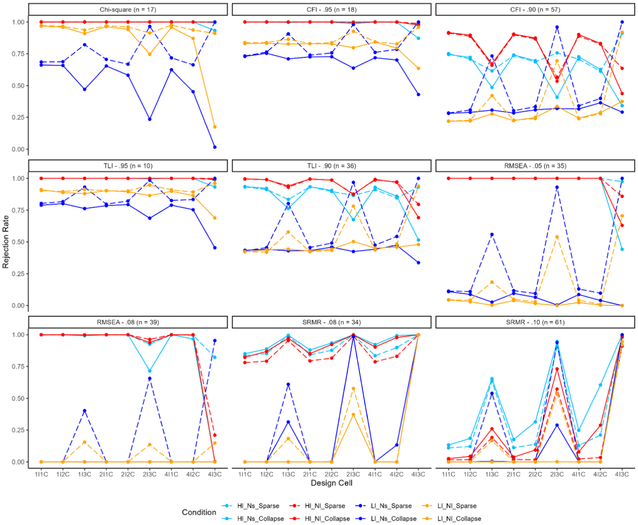
Model Rejection Rates Under Misspecified Model 1.

Figure 4.

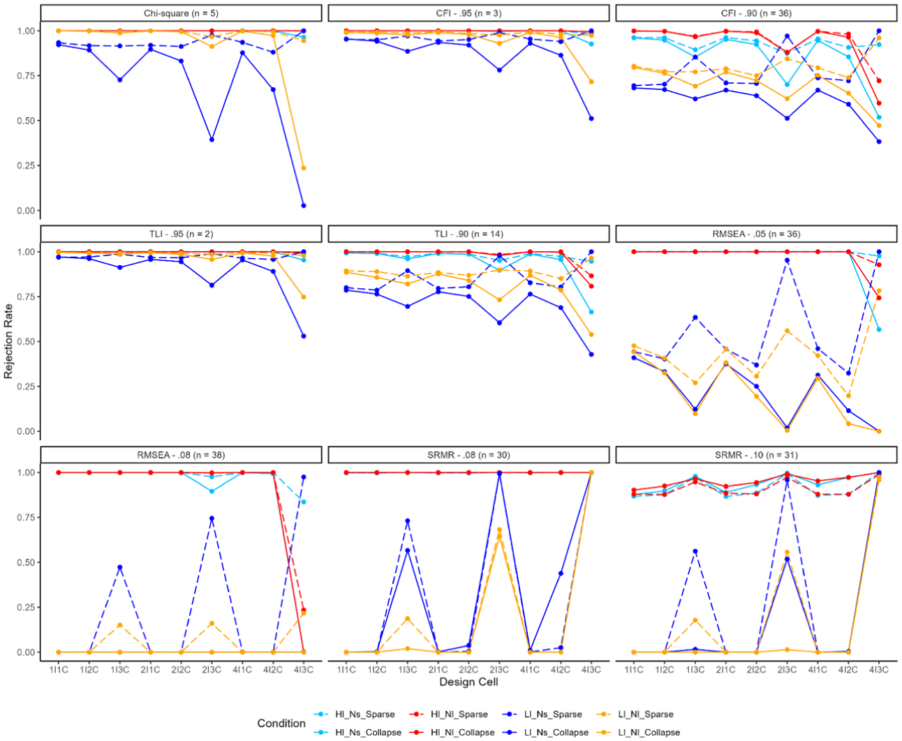
Model Rejection Rates Under Misspecified Model 2.

Model Rejection Under the Correctly Specified Model

Model rejections were examined for the correctly specified model (Figure 2). Collapsing data (solid lines) generally reduced model rejection rates while holding other conditions constant. Due to the varying patterns observed across different fit indices, the results were discussed separately. Inflated model rejection rates above .05 were commonly observed in conditions with sparse responses for chi-square statistics (51 out of 72 conditions). The number of response categories with sparse responses had a greater impact on model rejection rates than the number of items with sparse data. Low factor loadings and small sample sizes were linked with inflated model rejection rates. Collapsing responses effectively controlled model rejection rates (i.e., Type I error) under these conditions (average rejection rates from .235 to .044).

For CFI, the inflated model rejection rates were observed in 10 cells when the cut-off value was .90 and 27 cells when the cut-off value was .95 under all 72 conditions. Similar patterns were observed for TLI. When using a cut-off value of .95, 26 out of 72 cells demonstrated inflated model rejection rates, particularly in cases with low-factor loadings and a sample size of 250. In addition, 15 out of 72 cells exhibited model rejection rates exceeding .05, mainly under conditions with three sparse categories for a cut-off value of .90. Collapsing responses resulted in model rejection rates below .05 in most conditions when using the two cut-off values for both TLI and CFI, except for conditions with a small sample size of 250, low factor loadings of .5, and a cut-off value of .95. This aligned the average model rejection rates for both indices.

Finally, inflated model rejection rates existed in conditions with three sparse categories, and patterns were similar between the two cut-off values for RMSEA (10 out of 72 cells). Collapsing responses effectively controlled the model rejection rates to 0, and varying the cut-off values did not significantly impact the model rejection rates. Similarly, for SRMR, inflated model rejection rates occurred when there were three response categories with sparse responses under both cut-off values (N = 19 or 16). However, when combined with four items exhibiting sparse responses, SRMR displayed extremely high model rejection rates, and collapsing responses failed to mitigate the issue (Figure 2). Across all fit indices, conditions with high-factor loadings and small sample sizes yielded the highest model rejection rates at all levels of sparsity.

Model Rejection Under the Mild Misspecified Model (M1)

When models are misspecified, higher model rejection rates are desirable, as it reflects the fit indices’ effectiveness in identifying and rejecting poorly fitting models. Model rejection rates under the mild misspecified model (i.e., one item misloading on a different factor) were plotted in Figure 3, and the number of low model rejections below .80 was noted above each subfigure. First, low model rejection rates (<.80) were observed in approximately 10 to 20 out of 72 conditions (e.g., sample size of 250, low-factor loadings) for chi-square statistics, CFI (.95), and TLI (.95). When the cut-off value was .90, similar variations were observed for CFI and TLI. Low model rejection rates were more prevalent with a lower cut-off value. For instance, model rejection rates of CFI were low in most conditions (57 out of 72) with low loadings and/or low sample size (i.e., 250).

RMSEA and SRMR exhibited unique patterns compared to other fit indices. For RMSEA, low loadings had a major influence on model rejection rates across all conditions, and approximately half of the conditions displayed low model rejection rates under both cut-off values (35 or 39 out of 72 cells). SRMR was good at rejecting the model when the sparse levels were extremely high (i.e., four items and three responses) before and after collapsing, while SRMR cannot appropriately reject the model (i.e., low model rejection rates) in most other conditions, especially with a cut-off value of .10 (61 out of 72 cells).

Unfortunately, collapsing responses further lowered model rejection rates under certain conditions (Figure 3). For example, the rejection rate for RMSEA (cut-off = .05) decreased from .859 to .630 when the sample size was 500, factor loadings were .80, and four items with three sparse categories per factor were present. Similar patterns were observed for other fit indices. These results suggest that collapsing responses were not recommended, and that TLI was the most optimal index for maintaining acceptable model rejection rates (Figure 3).

Model Rejection Under the Severe Misspecified Model (M2)

Two factors were collapsed into one factor (Figure 1) in the severely specified model. Model rejection rates are presented in Figure 4, with the number of low model rejection rates (less than 0.80) noted below each subfigure. Collapsing responses reduced model rejection rates under these conditions. Model rejection was with minimal concern for chi-square statistics, CFI (.95), and TLI (.95) with frequencies ranging from 2 to 5. These fit indices can correctly reject the inappropriate model as long as no collapsing occurred. When the cut-off value was reduced to .90 for CFI, model rejection rates were significantly impacted by low factor loadings. In contrast, TLI performed better, maintaining model rejections within a reasonable range as long as responses were not collapsed. The results were aligned with the average model rejection rates (Table 3).

For RMSEA, low factor loadings had a substantial impact on model rejection across all conditions, with approximately half of the conditions showing low model rejection rates under both cut-off values (36 or 38 out of 72 cells). Similar patterns were observed for SRMR, except in conditions with severe sparse responses, where SRMR demonstrated high model rejection rates. While collapsing responses tended to reduce model rejection rates, the overall conclusion regarding high or low model rejection rates based on the cut-off value remained the same in most conditions.

Overall, collapsing responses reduced model rejection rates consistently, suggesting that it may lead to a higher likelihood of model acceptance under severely sparse conditions. The difference before and after collapsing was large in a few conditions with three categories of sparse responses (e.g., mild misspecified model, CFI: 90, sample size: 250, high loadings: .8, four items with sparse responses in three categories).

Stability of Fit Indices

The supplemental materials display the boxplots of CFI, TLI, RMSEA, and SRMR across all conditions. Overall, the estimates were stable, except for the conditions involving three categories with sparse responses. Collapsing responses led to an increase in RMSEA and SRMR and a decrease in CFI and TLI, increasing the stability of all four fit indices in such conditions. In addition, the correctly specified model produced more stable estimates compared to the misspecified models. Low factor loadings also contributed to decreased stability in TLI and CFI estimates.

Empirical Findings

Consistent with the simulation findings, when sparse responses were limited to a large number of items and a small number of categories (e.g., four items with one sparse response category), model decision (i.e., to retain or reject) was largely unaffected by data collapsing with minor variations (Table 4). However, model fit indices tended to improve under both correctly specified and misspecified models, aligning with the simulation results. In other words, data collapsing made it somewhat more likely for a model to be retained. For example, the CFI increased from .860 to .899, suggesting improved model fit following category collapsing. Finally, SRMR under the correctly specified model did not follow the same pattern as other fit indices, although the discrepancy was small (< .05).

Table 4.

Model Fit Indices of the Empirical Example.

Model fit	Correct		Misspecification
Model fit	Sparse	Collapse	Sparse	Collapse
Chi-square	112.714*	80.621*	1,021.566*	614.586*
RMSEA	.067	.064	.238	.182
CFI	.989	.992	.860	.899
TLI	.985	.989	.815	.866
SRMR	.042	.046	.116	.112

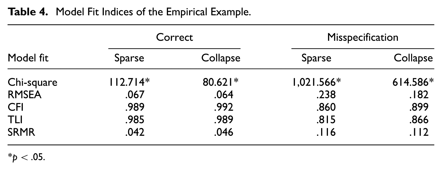
p < .05.

Discussion

The current study investigated the impact of infrequent collapsing to sparse ordinal data in CFA. Few prior studies have explored this issue, particularly under conditions involving model misspecification and its effect on rejection rates across various model fit indices. Data were simulated to vary sample size, factor loadings, sparseness levels, and model specification. In general, collapsing responses reduced the stability of fit estimates and model rejection rates when the variation was obvious in severely sparse conditions. Therefore, applied researchers must carefully weigh the benefits and risks of collapsing in practice.

First, the number of items exhibiting sparseness and item distribution of sparse items matter when considering collapsing responses for a scale (DiStefano et al., 2021). When there were one or two items with sparse responses on a factor and one or two sparse categories on these items, CFA models yielded relatively high convergence rates, decent model rejection rates, and stable fit indices. Importantly, the number of sparse categories had a greater influence on the model performance than the number of items exhibiting sparsity. One explanation is that sparseness was not fully recovered even after collapsing when there were sparse responses in three categories (from 94%, 2%, 2%, and 2% to 94% and 6%). In these conditions, item skewness (i.e., non-normality) causes inflated Type I error rates and low statistical power. In the current study, such problems were more pronounced when the sample size was small (i.e., 250) and factor loadings were low (i.e., .50). In those conditions, collapsing responses had obvious effects on various model fit indices.

In general, collapsing responses highlighted the improvement in convergence rates and Type I error rates under the correctly specified model (DiStefano et al., 2021), thereby mitigating issues caused by sparse data. Chi-square statistics were sensitive to sample sizes, with inflated model rejection rates (i.e., Type I error rates) above .05 in many cells (N = 51 out of 72). This sensitivity means that, particularly in large samples, even minor discrepancies between the observed data and the model can result in significant chi-square values, causing researchers to inappropriately reject correctly specified models (Alavi et al., 2020; Li, 2016). Consequently, applied researchers often encounter significant chi-square results and may choose to focus on alternative fit indices when selecting the optimal model.

RMSEA demonstrated the best performance in controlling model rejections for the correctly identified model, and collapsing responses completely resolved the concern of inflated model rejection rates. While CFI and TLI exhibited inflated model rejection rates in certain conditions, the conditions were mostly relieved by collapsing responses. However, with a stringent cut-off value of .95, low factor loadings, and a sample size of 250, all relevant conditions had inflated model rejection rates even after collapsing. Finally, model rejection rates of SRMR were out of control when the sparse levels were high, aligning with the conclusion that the accuracy of SRMR in controlling model rejection rates can be compromised in the presence of non-normal data (Pavlov et al., 2021). While collapsing responses reduced model rejection rates, conditions with four sparse items in three response categories had extremely high model rejection rates indicating that researchers are likely to reject the correctly identified model for SRMR.

Meanwhile, the simulation findings also highlighted the trade-off of increased risk in investigating misspecified models. Collapsing response uniformly reduced model rejections. Comparing two model misspecifications, the fit indices demonstrated lower model rejection rates overall when the model was mildly misspecified with one item misloaded on a different factor. This aligns with prior studies concluding different abilities to identify different levels of misspecification in CFA (e.g., DiStefano et al., 2018). In other words, it was relatively difficult to reject inappropriate models when they were a minor misspecification (McIntosh, 2012). Overall, chi-square, CFI, and TLI were superior to addressing model rejections under misspecified models than RMSEA and SRMR; a cut-off value of .95 was recommended for CFI and TLI as the threshold to filter out most under-factored models (Clark & Bowles, 2018) without collapsing responses.

RMSEA showed low model rejection rates with about half of the conditions due to low factor loadings. This is consistent with findings that the recovery of low factor loadings is poor in misspecified models (Ximénez, 2006) and that RMSEA is less sensitive to different types of model misspecification (Savalei, 2012). In contrast to its poor performance in controlling model rejection rates in the correctly identified model, SRMR effectively rejected incorrect models in severely sparse conditions. However, SRMR is not recommended for use in other conditions. For instance, under mildly misspecified models, SRMR exhibited low model rejection rates in 61 out of 72 cells. Moreover, based on the cut-off value of .8, the model rejection decision did not vary significantly before and after collapsing for both RMSEA and SRMR indicating the low sensitivity in data collapsing.

Examining the two sets of cut-off values results revealed that CFI and TLI were sensitive to the chosen cut-off values in response to data collapsing. A stringent cut-off of .95 led to elevated model rejection rates, which suggests that one fixed cut-off value may not be enough in practice (Groskurth et al., 2024). In contrast, RMSEA was not influenced by the cut-off values, yielding consistent conclusions regardless of the threshold. SRMR showed only a mild sensitivity to cut-off values under the mildly misspecified model, where a stringent cut-off of .08 was associated with increased model rejection rates.

Recommendations for Researchers

In the scale design phase, researchers should anticipate potential sparse response patterns and consider the need for collapsing responses. A preliminary step is to compute frequencies of each item on a scale to investigate potential sparse responses in pilot studies. While there are no definitive guidelines for applied researchers to select the best model fit, collapsing sparse responses offers potential benefits but involves trade-offs that must be carefully evaluated. While it is well-known that researchers should be cautious about rejecting a correctly specified model based on chi-square statistics (Alavi et al., 2020) in larger samples, chi-square statistics remain valuable for model selection, particularly in rejecting severely misspecified models under most conditions.

Recent studies have emphasized the importance of reporting chi-square statistics alongside other fit indices to provide a comprehensive assessment of model performance (Zheng & Bentler, 2024). However, it is common to have disagreement among fit indices due to their variations in theories (Lai & Green, 2016); thus, it is necessary to refer to different indices for different occasions. Based on our study findings, we recommend the use of RMSEA to address model rejections under the correctly identified model, while TLI with a cut-off value of .95 is suggested to address model rejections under the misspecified models. When high levels of sparsity exist, with many items having sparse responses across most categories, SRMR can be a useful indicator for identifying inappropriate models.

The empirical results were aligned with the simulation results in the current study and prior literature (DiStefano et al., 2021). In general, if the number of sparse response categories is low, maintaining the original categorical structure may be preferable, since model conclusions are unlikely to change due to collapsing. In addition to model fit differences before and after collapsing, such changes can alter the underlying meaning of response options. Such modifications to the scale format may affect how scores are interpreted, making results from different versions of the scale not directly comparable (Cabooter et al., 2016). Researchers applying category collapsing during data cleaning should avoid comparison of different versions of the same scale with different response structures unless measurement invariance has been established.

Limitations and Future Research Directions

First, the simulation conditions tested in the current study were predetermined based on researchers’ judgments, and we recognized that the findings were not generalizable to other conditions that were not tested here. Future studies could expand upon this work by incorporating additional simulation conditions to examine whether similar conclusions are reached. For instance, the current study employed four response categories; however, prior research has shown that the RMSEA is sensitive to the number of response categories (Monroe & Cai, 2015), suggesting that this factor could be varied in future studies. The current study focuses on two types of misspecified models, leaving other conditions, such as over-factored models (Clark & Bowles, 2018), to be explored. In addition, the current study only investigated a limited approach to item-level sparseness. Future research should consider more comprehensive frameworks for defining sparseness, including the location of sparseness within the scale and the distributional characteristics across items (Rutkowski et al., 2019; Tsai et al., 2024).

Model estimation methods could impact the performance of model fit (DiStefano et al., 2021; Shi et al., 2019). Modeling with different estimation methods can provide complementary information for researchers. Thus, this can be addressed in future studies. The popularity of treating Likert-type scale data as continuous variables is common in practice. Future research should consider incorporating ML-based methods. Our study did not explore the usage of more advanced estimation methods, such as Bayesian estimation, which have been shown to perform well under conditions of sparse categorical data structures (e.g., Bainter, 2017; Liang & Yang, 2014). The techniques employed in this study were intentionally selected with applied researchers in mind, recognizing that practitioners may face challenges in navigating the complexities of advanced methods, such as determining appropriate prior probabilities for Bayesian analyses (DiStefano et al., 2021). Future simulation studies could benefit from incorporating such methods.

In addition, while this study focused on a typical factor model, other CFA models, such as higher-order factor models and bifactor models, are also widely used in applied research (Morgan et al., 2015). Their performance under data conditions remains unclear. Future research should investigate the performance related to data sparsity to extend the findings in the current study.

Traditional cut-off scores were utilized to evaluate model rejection rates across simulation conditions. While this is a well-accepted practice, we admitted the limitations of overgeneralizing cut-off scores, especially for ordinal data (Monroe & Cai, 2015). Future research could integrate the Direct Discrepancy Dynamic (DDD) Fit Index framework (McNeish & Wolf, 2024) to complement traditional fixed cut-offs when evaluating model performance under sparse data conditions. In short, the DDD approach generates fit thresholds empirically for each model and dataset, which could provide more accurate evaluations of model rejection.

Finally, missing data is a common issue in research (Mirzaei et al., 2022) and often complicates scale analysis. When combined with sparse data, these challenges can become even more difficult to manage. While the current study solely focused on sparse data, future research could address both issues simultaneously to better understand their combined impact on model performance, which will provide practical guidance for researchers handling complex data situations (Jeong & Lee, 2016).

In summary, this study underscores the impact of collapsing sparse response categories in Likert-type scale data on the model fit of CFA. The findings highlight that such data collapsing can reduce model rejections in both correctly specified and misspecified models, with varying responses observed across different fit indices. These insights provide valuable guidance for researchers navigating issues relevant to sparse data.

Supplemental Material

sj-docx-1-epm-10.1177_00131644251401097 – Supplemental material for Collapsing Sparse Responses in Likert-Type Scale Data: Advantages and Disadvantages for Model Fit in CFA

Supplemental material, sj-docx-1-epm-10.1177_00131644251401097 for Collapsing Sparse Responses in Likert-Type Scale Data: Advantages and Disadvantages for Model Fit in CFA by Jin Liu, Yu Bao, Christine DiStefano and Wei Jiang in Educational and Psychological Measurement

Footnotes

Declaration of Conflicting Interests

The authors declared no potential conflicts of interest with respect to the research, authorship, and/or publication of this article.

Funding

The authors received no financial support for the research, authorship, and/or publication of this article.

ORCID iDs

Jin Liu

Yu Bao

Christine DiStefano

Supplemental Material

Supplemental material for this article is available online.

References

Alavi

Visentin

D. C.

Thapa

D. K.

Hunt

G. E.

Watson

Cleary

(2020). Chi-square for model fit in confirmatory factor analysis. Journal of Advanced Nursing, 76(9), 2209–2211. https://doi.org/10.1111/jan.14399

Aybek

E. C.

Toraman

(2022). How many response categories are sufficient for Likert-type scales? An empirical study based on the Item Response Theory. International Journal of Assessment Tools in Education, 9(2), 534–547. https://doi.org/10.21449/ijate.1132931

Bainter

S. A.

(2017). Bayesian estimation for item factor analysis models with sparse categorical indicators. Multivariate Behavioral Research, 52(5), 593–615. https://doi.org/10.1080/00273171.2017.1342203

Bowden

Singh

Thompson

Gonzalez

Katz

Dahl

Prihoda

Chang

(2007). Development of the bipolar inventory of symptoms scale. Acta Psychiatrica Scandinavica, 116(3), 189–194. https://doi.org/10.1111/j.1600-0447.2006.00955.x

Brown

T. A.

(2015). Confirmatory factor analysis for applied research (2nd ed.). The Guilford Press.

Cabooter

Weijters

Geuens

Vermeir

(2016). Scale format effects on response option interpretation and use. Journal of Business Research, 69(7), 2574–2584. https://doi.org/10.1016/j.jbusres.2015.10.138

Chen

Curran

P. J.

Bollen

K. A.

Kirby

Paxton

(2008). An empirical evaluation of the use of fixed cutoff points in RMSEA test statistic in structural equation models. Sociological Methods & Research, 36(4), 462–494. https://doi.org/10.1177/0049124108314720

Clark

D. A.

Bowles

R. P.

(2018). Model fit and item factor analysis: Overfactoring, underfactoring, and a program to guide interpretation. Multivariate Behavioral Research, 53(4), 544–558. https://doi.org/10.1080/00273171.2018.1461058

Cohen

(1988). Statistical power for the behavioral sciences. Lawrence Erlbaum.

10.

Colvin

K. F.

Gorgun

(2020). Comparing interpretations of the Rosenberg Self-Esteem Scale with 4-, 5-, and 101-point scales. Practical Assessment, Research & Evaluation, 38(6), 762–766. https://doi.org/10.1177/0734282920915063

11.

Davis

C. G.

Thake

Vilhena

(2010). Social desirability biases in self-reported alcohol consumption and harms. Addictive Behaviors, 35(4), 302–311. https://doi.org/10.1016/j.addbeh.2009.11.001

12.

DiStefano

(2016). Examining fit with structural equation models. In Schweizer

DiStefano

(Eds.), Psychological assessment – science and practice: Principles and methods of test construction: Standards and recent advances (Vol.3, 120, pp. 166–193). Hogrefe Publishing.

13.

DiStefano

Liu

Jiang

Shi

(2018). Examination of the weighted root mean square residual: Evidence for trustworthiness? Structural Equation Modeling: A Multidisciplinary Journal, 25(3), 453–466. https://doi.org/10.1080/10705511.2017.1390394

14.

DiStefano

Morgan

G. B.

(2014). A comparison of diagonal weighted least squares robust estimation techniques for ordinal data. Structural Equation Modeling: A Multidisciplinary Journal, 21(3), 425–438. https://doi.org/10.1080/10705511.2014.915373

15.

DiStefano

Shi

Morgan

G. B.

(2021). Collapsing categories is often more advantageous than modeling sparse data: Investigations in the CFA framework. Structural Equation Modeling: A Multidisciplinary Journal, 28(2), 237–249. https://doi.org/10.1080/10705511.2020.1803073

16.

Eichhorn

(2022). Survey research and sampling. Sage.

17.

Finney

S. J.

DiStefano

(2013). Nonnormal and categorical data in structural equation modeling. In Hancock

G. R.

Mueller

R. O.

(Eds.), Structural equation modeling: A second course (2nd ed., pp. 439–492). IAP Information Age Publishing.

18.

Forsyth

D. R.

(1980). A taxonomy of ethical ideologies. Journal of Personality and Social Psychology, 39(1), 175. https://doi.org/10.1037//0022-3514.39.1.175

19.

Gagné

Hancock

G. R.

(2006). Measurement model quality, sample size, and solution propriety in confirmatory factor models. In Hancock

G. R.

Mueller

R. O.

(Eds.), Structural equation modeling: A second course (pp. 101–124). IAP Information Age Publishing.

20.

Goretzko

Siemund

Sterner

(2024). Evaluating model fit of measurement models in confirmatory factor analysis. Educational and Psychological Measurement, 84(1), 123–144. https://doi.org/10.1177/00131644231163813

21.

Grimbeek

Bryer

Beamish

D’Netto

. (2005, January). Use of data collapsing strategies to identify latent variables in CHP questionnaire data. In Bartlett

Bryer

Roebuck

(Eds.), Proceedings of 3rd international conference on cognition, language, and special education (pp. 125–139). Griffith Research Online.

22.

Groskurth

Bluemke

Lechner

C. M.

(2024). Why we need to abandon fixed cutoffs for goodness-of-fit indices: An extensive simulation and possible solutions. Behavior Research Methods, 56(4), 3891–3914. https://doi.org/10.3758/s13428-023-02193-3

23.

Horan

P. M.

DiStefano

Motl

R. W.

(2003). Wording effects in self-esteem scales: Methodological artifact or response style? Structural Equation Modeling, 10(3), 435–455. https://doi.org/10.1207/S15328007SEM1003_6

24.

L. T.

Bentler

P. M.

(1999). Cutoff criteria for fit indexes in covariance structure analysis: Conventional criteria versus new alternatives. Structural Equation Modeling: A Multidisciplinary Journal, 6(1), 1–55. https://doi.org/10.1080/10705519909540118

25.

Jeong

H. J.

Lee

W. C.

(2016). The level of collapse we are allowed: Comparison of different response scales in Safety Attitudes Questionnaire. Biometrics & Biostatistics International Journal, 4(4), 128–134. http://doi.org/10.15406/bbij.2016.04.00100

26.

Joshi

Kale

Chandel

Pal

(2015). Likert scale: Explored and explained. British Journal of Applied Science & Technology, 7(4), 396–403. https://doi.org/10.9734/bjast/2015/14975

27.

Kankaraš

Capecchi

(2024). Neither agree nor disagree: Use and misuse of the neutral response category in Likert-type scales. METRON, 83, 111–140. https://doi.org/10.1007/s40300-024-00276-5

28.

Kline

R. B.

(2011). Principles and practice of structural equation modeling (3rd ed.). The Guilford Press.

29.

Lai

Green

S. B.

(2016). The problem with having two watches: Assessment of fit when RMSEA and CFI disagree. Multivariate Behavioral Research, 51(2–3), 220–239. https://doi.org/10.1080/00273171.2015.1134306

30.

Lee

Paek

(2014). In search of the optimal number of response categories in a rating scale. Journal of Psychoeducational Assessment, 32(7), 663–673. https://doi.org/10.1177/0734282914522200

31.

C. H.

(2016). Confirmatory factor analysis with ordinal data: Comparing robust maximum likelihood and diagonally weighted least squares. Behavior Research Methods, 48(3), 936–949. https://doi.org/10.3758/s13428-015-0619-7

32.

Liang

Yang

(2014). An evaluation of WLSMV and Bayesian methods for confirmatory factor analysis with categorical indicators. International Journal of Quantitative Research in Education, 2(1), 17–38. https://doi.org/10.1504/ijqre.2014.060972

33.

Liu

Harbaugh

A. G.

Harring

J. R.

Hancock

G. R.

(2017). The effect of extreme response and non-extreme response styles on testing measurement invariance. Frontiers in Psychology, 8, 726. https://doi.org/10.3389/fpsyg.2017.00726

34.

Lozano

L. M.

García-Cueto

Muñiz

(2008). Effect of the number of response categories on the reliability and validity of rating scales. Methodology, 4(2), 73–79. https://doi.org/10.1027/1614-2241.4.2.73

35.

MacCallum

R. C.

Browne

M. W.

Sugawara

H. M.

(1996). Power analysis and determination of sample size for covariance structure modeling. Psychological Methods, 1(2), 130–149. https://doi.org/10.1037/1082-989x.1.2.130

36.

Matell

M. S.

Jacoby

(1971). Is there an optimal number of alternatives for Likert scale items? Study 1: Reliability and validity. Educational and Psychological Measurement, 31, 657–674. https://doi.org/10.1177/001316447103100307

37.

Maydeu-Olivares

Fairchild

A. J.

Hall

A. G.

(2017). Goodness of fit in item factor analysis: Effect of the number of response alternatives. Structural Equation Modeling: A Multidisciplinary Journal, 24(4), 495–505. https://doi.org/10.1080/10705511.2017.1289816

38.

McIntosh

C. N.

(2012). Improving the evaluation of model fit in confirmatory factor analysis: A commentary on Gundy, C. M., Fayers, P.M., Groenvold, M., Petersen, M. Aa., Scott, N.W., Sprangers, M.A.J., Velikov, G., Aaronson, N.K. (2011). Comparing higher-order models for the EORTC QLQ-C30. Quality of Life Research. doi:10.1007/s11136-011-0082-6. Quality of Life Research, 21(9), 1619–1621. https://doi.org/10.1007/s11136-011-0084-4

39.

McNeish

Wolf

M. G.

(2024). Direct discrepancy dynamic fit index cutoffs for arbitrary covariance structure models. Structural Equation Modeling: A Multidisciplinary Journal, 31(5), 835–862. https://doi.org/10.1080/10705511.2024.2308005

40.

Mirzaei

Carter

S. R.

Patanwala

A. E.

Schneider

C. R.

(2022). Missing data in surveys: Key concepts, approaches, and applications. Research in Social and Administrative Pharmacy, 18(2), 2308–2316. https://doi.org/10.1016/j.sapharm.2021.03.009

41.

Monroe

Cai

(2015). Evaluating structural equation models for categorical outcomes: A new test statistic and a practical challenge of interpretation. Multivariate Behavioral Research, 50(6), 569–583. https://doi.org/10.1080/00273171.2015.1032398

42.

Morgan

G. B.

Hodge

K. J.

Wells

K. E.

Watkins

M. W.

(2015). Are fit indices biased in favor of bi-factor models in cognitive ability research? A comparison of fit in correlated factors, higher-order, and bi-factor models via Monte Carlo simulations. Journal of Intelligence, 3(1), 2–20. https://doi.org/10.3390/jintelligence3010002

43.

Moshagen

Musch

(2014). Sample size requirements of the robust weighted least squares estimator. Methodology, 10(2), 60–70. https://doi.org/10.1027/1614-2241/a000068

44.

Muthén

L. K.

Muthén

B. O.

(2017). Mplus user’s guide (8th ed.). Muthén & Muthén.

45.

Nemoto

Beglar

(2014). Likert-scale questionnaires. In Sonda

Krause

(Eds.), JALT 2013 conference proceedings (pp. 1–8). JALT.

46.

Oaster

T. R. F.

(1989). Number of alternatives per choice point and stability of Likert-type scales. Perceptual and Motor Skills, 68, 549–550.

47.

O’Boyle

E. H.

Forsyth

D. R.

(2021). Individual differences in ethics positions: The EPQ-5. PLOS ONE, 16(6), e0251989. https://doi.org/10.1371/journal.pone.0251989

48.

Pavlov

Maydeu-Olivares

Shi

(2021). Using the standardized root mean squared residual (SRMR) to assess exact fit in structural equation models. Educational and Psychological Measurement, 81(1), 110–130. https://doi.org/10.1177/0013164420926231

49.

Preston

C. C.

Colman

A. M.

(2000). Optimal number of response categories in rating scales: Reliability, validity, discriminating power, and respondent preferences. Acta Psychologica, 104(1), 1–15. https://doi.org/10.1016/s0001-6918(99)00050-5

50.

Revilla

M. A.

Saris

W. E.

Krosnick

J. A.

(2014). Choosing the number of categories in agree–disagree scales. Sociological Methods & Research, 43(1), 73–97. https://doi.org/10.1177/0049124113509605

51.

Rhemtulla

Brosseau-Liard

P. É.

Savalei

(2012). When can categorical variables be treated as continuous? A comparison of robust continuous and categorical SEM estimation methods under suboptimal conditions. Psychological Methods, 17(3), 354–373. https://doi.org/10.1037/a0029315

52.

Rutkowski

Svetina

Liaw

Y.-L.

(2019). Collapsing categorical variables and measurement invariance. Structural Equation Modeling, 26(5), 790–802. https://doi.org/10.1080/10705511.2018.1547640

53.

Savalei

(2011). What to do about zero frequency cells when estimating polychoric correlations. Structural Equation Modeling, 18(2), 253–273. https://doi.org/10.1080/10705511.2011.557339

54.

Savalei

(2012). The relationship between root mean square error of approximation and model misspecification in confirmatory factor analysis models. Educational and Psychological Measurement, 72(6), 910–932. https://doi.org/10.1177/001316441245256

55.

Shi

Lee

Maydeu-Olivares

(2019). Understanding the model size effect on SEM fit indices. Educational and Psychological Measurement, 79(2), 310–334. https://doi.org/10.1177/0013164418783520

56.

Shi

Maydeu-Olivares

(2020). The effect of estimation methods on SEM fit indices. Educational and Psychological Measurement, 80(3), 421–445. https://doi.org/10.1177/0013164419885164

57.

Sullivan

G. M.

Artino

A. R.

(2013). Analyzing and interpreting data from Likert-type scales. Journal of Graduate Medical Education, 5(4), 541–542. https://doi.org/10.4300/jgme-5-4-18

58.

Tsai

C.-L.

Wind

Estrada

(2024). Exploring the effects of collapsing rating scale categories in polytomous item response theory analyses: An illustration and simulation study. Measurement: Interdisciplinary Research and Perspectives, 23(1), 66–89. https://doi.org/10.1080/15366367.2023.2288791

59.

Wang

Liu

DiStefano

Pan

Gao

Tang

(2021). Utilizing deep learning and oversampling methods to identify children’s emotional and behavioral risk. Journal of Psychoeducational Assessment, 39(2), 227–241. https://doi.org/10.1177/0734282920950370

60.

Winrow

A. R.

Reitmaier-Koehler

Winrow

B. P.

(2015). Social desirability bias in relation to academic cheating behaviors of nursing students. Journal of Nursing Education and Practice, 5(8), 121–128. https://doi.org/10.5430/jnep.v5n8p121

61.

Wolf

E. J.

Harrington

K. M.

Clark

S. L.

Miller

M. W.

(2013). Sample size requirements for structural equation models: An evaluation of power, bias, and solution propriety. Educational and Psychological Measurement, 73(6), 913–934. https://doi.org/10.1177/0013164413495237

62.

Xia

Yang

(2019). RMSEA, CFI, and TLI in structural equation modeling with ordered categorical data: The story they tell depends on the estimation methods. Behavior Research Methods, 51(1), 409–428. https://doi.org/10.3758/s13428-018-1055-2

63.

Ximénez

(2006). A Monte Carlo study of recovery of weak factor loadings in confirmatory factor analysis. Structural Equation Modeling, 13(4), 587–614. https://doi.org/10.1207/s15328007sem1304_5

64.

Yang

T. R.

Weng

L. J.

(2024). Revisiting Savalei’s (2011) research on remediating zero-frequency cells in estimating polychoric correlations: A data distribution perspective. Structural Equation Modeling, 31(1), 81–96. https://doi.org/10.1080/10705511.2023.2220919

65.

Zhao

Zheng

Zhao

Compton

B. J.

Zhang

Fang

Heyman

G. D.

Lee

(2023). Cheating among elementary school children: A machine learning approach. Child Development, 94(4), 922–940. https://doi.org/10.1111/cdev.13910

66.

Zheng

B. Q.

Bentler

P. M.

(2024). Enhancing model fit evaluation in SEM: Practical tips for optimizing chi-square tests. Structural Equation Modeling: A Multidisciplinary Journal. Advance online publication. https://doi.org/10.1080/10705511.2024.2354802

Supplementary Material

Please find the following supplemental material available below.

For Open Access articles published under a Creative Commons License, all supplemental material carries the same license as the article it is associated with.

For non-Open Access articles published, all supplemental material carries a non-exclusive license, and permission requests for re-use of supplemental material or any part of supplemental material shall be sent directly to the copyright owner as specified in the copyright notice associated with the article.

0.00 MB

0.44 MB