
Abstract
The problem of local item dependencies (LIDs) is very common in personality and attitude measures, particularly in those that measure narrow-bandwidth dimensions. At the structural level, these dependencies can be modeled by using extended factor analytic (FA) solutions that include correlated residuals. However, the effects that LIDs have on the scores based on these extended solutions have received little attention so far. Here, we propose an approach to simple sum scores, designed to assess the impact of LIDs on the accuracy and effectiveness of the scores derived from extended FA solutions with correlated residuals. The proposal is structured at three levels—(a) total score, (b) bivariate-doublet, and (c) item-by-item deletion—and considers two types of FA models: the standard linear model and the nonlinear model for ordered-categorical item responses. The current proposal is implemented in SINRELEF.LD, an R package available through CRAN. The usefulness of the proposal for item analysis is illustrated with the data of 928 participants who completed the Family Involvement Questionnaire-High School Version (FIQ-HS). The results show not only the distortion that the doublets cause in the omega reliability estimate when local independency is assumed but also the loss of information/efficiency due to the local dependencies.
Keywords
Throughout its long history, the problem of related specificities among the items that form a scale has been largely addressed by three different frameworks. First, since the 1920s, Classical Test Theory (CTT) has considered the problem mainly at the score level and focused on how it affects the bias in the reliability estimate (Guilford, 1936; Kelley, 1924; Sireci et al., 1991). Second, factor analysis (FA) refers to the problem as “correlated residuals” or “doublets” (Mulaik, 2010; Thurstone, 1947) and is mainly concerned with the structural distortions that these related specificities can produce in the FA solution (Ferrando et al., 2024; Mulaik, 2010). Finally, Item Response Theory (IRT) takes a broader focus and considers potential bias in (a) the item parameter estimates, (b) the score estimates, and (c) the measures of accuracy and information (Chen & Thissen, 1997; Sireci et al., 1991; Wang & Wilson, 2005; Yen, 1993). Psychometric considerations aside, substantive aspects should also be taken into account when addressing the problem because the causes, forms, and impact of the local item dependencies (LIDs) are generally different in cognitive and noncognitive measurement (Bandalos, 2021; DeMars, 2020; Yen, 1993). Cognitive measures assess cognitive abilities or proficiencies such as reasoning, attention, memory, language, and so on. Some of these measures limit the response time, and if it is insufficient, the items at the end of the test may be locally dependent (e.g., Yen, 1993). Locally dependent items may also be caused by practice (e.g., Yen, 1993). In addition, in some measures of this type, bundles or testlets of items are interconnected (and so, locally dependent) by design (e.g., when a set of questions is derived from a single common stimulus). In noncognitive measures (personality questionnaires, belief or attitude measures, and so on), however, time limitations and practice are much less relevant, the testlet design is uncommon, and the local dependence usually comes from other sources such as the ones discussed below.
Given the extent of the aforementioned problem, we shall first delimit the framework, focus, and potential applicability of what we propose here. At the psychometric level, we shall use results and principles from the three frameworks mentioned earlier: CTT, FA, and IRT. However, we shall be using FA as the general overarching model (e.g., McDonald, 1985). Furthermore, we shall (a) discuss only unidimensional measures, (b) focus mainly on the scoring stage, and (c) base the proposal on the simple sum scores. At the substantive level, our proposal is expected to be particularly suitable for analyzing personality and attitude measures. Finally, as far as terminology is concerned, we shall use the terms “correlated residuals,”“correlated specificities,”“doublets,” and “LIDs” indistinctly, although we are aware that the last term is more common than the others (probabilistic dependence vs. linear dependence; see, e.g., McDonald, 1982 or Yen, 1993).
We shall now provide (a) a brief justification for the choice of sum scores and (b) a discussion of the problem of LIDs in noncognitive domains. As for the first issue, in theory, the “best” option for scoring in scales derived from a unidimensional FA solution is factor score estimates (or predictors) that use all the information available in the estimated structural solution (e.g., Beauducel & Leue, 2013; Comrey & Lee, 1992; Ferrando & Lorenzo-Seva, 2021). So, provided that the FA solution on which they are based is appropriate and strong, the sum scores can be viewed as sub-optimal proxies for the factor score estimates, and the use of these scores unavoidably entails a loss of accuracy and information (Raykov et al., 2015). On the other hand, however, and in the scenario we are considering, the simple sum scores have interesting and nonnegligible properties. To start with, they are possibly the most widely used scoring procedure in psychometric applications (e.g., Raykov & Marcoulides, 2011) because they are easy to compute, interpret, and relate to previous studies (e.g., Grice & Harris, 1998; Widaman & Revelle, 2023). They can also provide more stable results under cross-validation (Grice & Harris, 1998; Wainer, 1976). With particular reference to the present proposal, and as shown below, the sum scores do not add additional biases to the trait estimates when there are correlated residuals (see also Yen, 1993). So, overall, we believe that what we propose here is of clear practical interest.
Turning now to the second issue, LIDs mainly occur in noncognitive measures for the following reasons: (a) repeated presentation of the same items, (b) similarities in content or wording, (c) similarities in the evoked situation, and (d) context effects (Bandalos, 2021; DeMars, 2020; Edwards et al., 2018; Ferrando & Morales-Vives, 2023). These four reasons suggest that the expected sign of the residual correlation will be positive (i.e., the respondent will tend to answer the pair of items in the same way, beyond the influence of the common factor that underlies them both). Residual correlations might also be negative, and in fact, this is what tends to occur in scales that contain items that are positively and negatively worded or keyed (Viladrich et al., 2017). In our view, however, these negative correlations are caused more by the systematic factors that have not been accounted for in the solution (e.g., method effects or acquiescence) than by “true” correlated specificities (Marsh, 1996; Viladrich et al., 2017). We should point out that production of correlated residuals by unmodeled factors is a scenario we shall not consider in this article (see S. B. Green & Hershberger, 2000).
Aims and Contributions
In this article, we propose an approach for assessing the accuracy and effectiveness of item and test scores obtained from unidimensional scales that contain local dependencies. The approach has three score levels: (a) total test, (b) bivariate-doublet, and (c) single item. It consists of a series of indices based on the two most general indices of measurement accuracy in psychometrics: reliability and information (e.g., Mellenbergh, 1996; Nicewander, 1993). The interpretation of both indices is discussed below in detail. As an initial summary, however, information is a signal/noise index that has no upper bound and is more suited to detecting changes due to local dependences at higher levels of accuracy, whereas reliability is a unitless measure with a unit upper bound that has a clearer interpretation. So, both measures complement each other very well for the purposes of the proposal. Finally, all the proposed indices are developed for calibration scenarios that use one of the following two FA models (e.g., McDonald, 1985): the linear model, in which the item scores are treated as (approximately) continuous, and the nonlinear underlying variables approach (UVA) FA in which they are treated as ordered categorical.
We believe that this study has contributed some results of theoretical interest, particularly in the case of UVA-FA. However, we consider that its main contributions are practical and instrumental. To appraise the practical relevance of what we propose here, however, some background considerations are in order. As further discussed below, a structural FA solution that includes correlated residuals can be routinely fitted at present. Furthermore, if this solution is reasonably correct, the biases in the loading and error item estimates that invariably occur when the related specificities are left unmodeled can be avoided (Ferrando et al., 2023). So, the correlated-residuals solution will provide an appropriate view of the quality of the individual items as measures of the construct (Mulaik, 2010). At the same time, however, this solution is more parameterized, complex, and potentially unstable than a classical FA solution with a diagonal residual matrix (Bandalos, 2021; MacCallum et al., 1992).
Consider now the estimation of individual scores using the structural solution that has been fitted. The presence of local dependencies will generally lead to item and test scores that are less accurate and informative even when they are based on a correct structural solution with correlated residuals. Furthermore, it seems that no procedure for making a detailed assessment of the extent of score accuracy and effectiveness lost due to local dependencies, such as the one we discuss here, has been proposed to date. So, we expect our proposal to be particularly useful in item analysis, as it will allow practitioners to (a) make a detailed assessment of the extent of accuracy and effectiveness lost due to local dependencies and (b) decide which items are to be kept to optimize the solution-complexity vs information-loss trade-off.
As for the contributions at the instrumental level, all the indices and procedures proposed in this article have been implemented in a noncommercial program that is described below and freely available to interested readers.
Indices Based on Linear FA Solutions
Consider a scale of j = 1 … n items, intended to measure a single trait or common factor θ, whose scores behave according to the unidimensional (Spearman) linear FA model. For a randomly selected respondent i that belongs to the population in which the FA solution holds, the basic FA equation for the item scores in scalar form is:

where X ij is the observed item score, µ j is an intercept term, λ j is the item loading, θ i is the trait level of the respondent, ψ j is the item residual standard deviation, and ε ij is a latent residual or error score. Both the common factor and the residual scores are in standard scale (zero mean and unit variance) and are assumed to be uncorrelated with each other. The items in Equation 1 are allowed to have different structural parameter values (intercepts, loadings, and residual variances) and are commonly known as congeneric (Jöreskog, 1971; Mellenbergh, 1996). To avoid unnecessary complexities, we shall assume that the items are all keyed in the same direction of θ and that all the loadings in Equation 1 are positive.
For subsequent developments, the vector-matrix notation should also be used. So, let

where

where

In psychometric applications, a structural model of type given in Equation 4 is usually fitted using a two-stage (calibration and scoring), random-regressor approach (McDonald, 1982). In the calibration stage, the structural parameters (intercepts, loadings, and residual variances) are estimated, and the goodness-of-model data fit is assessed. If the fit is acceptable and the solution is strong and stable, the structural estimates are taken as fixed and known and used as a basis for obtaining individual scores. At present, procedures are also available for calibrating the extended model (Equation 3), which includes the residual correlations as additional parameters. Some of them require the salient correlated residuals to be specified a priori (e.g., Exploratory Structural Equation Modelling; Asparouhov & Muthén, 2023, or efast; van Kesteren & Kievit, 2021), while in others, the salient doublets are obtained analytically (Ferrando et al., 2023). In all cases, we assume that a strong and well-fitting solution of type given in Equation 3 has been attained, and we shall focus only on the properties of the sum scores derived from it.
Let X be the simple (unit weight) sum score. According to Equation 1, we have
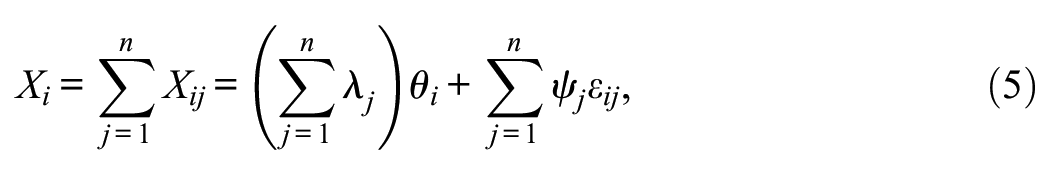
with conditional expectation and variance given by

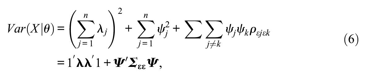
where
If Lord’s (1980) definition of the score information function is used, the information contributed by the sum score X as implied by the model in Equation 1 is found to be:
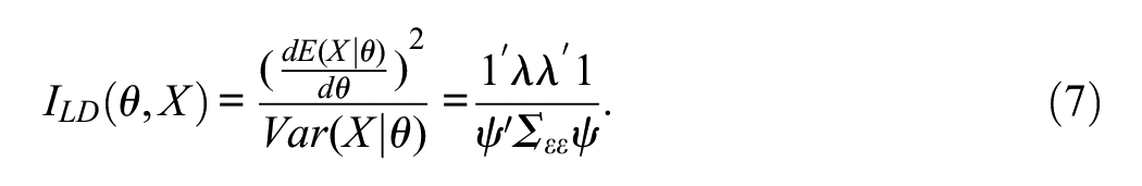
If the sum score is used to estimate the “true”θ level, then the measure (Equation 7) will be inversely proportional to the squared standard error of measurement and, therefore, to the width of the confidence interval (CI) for estimating θ from the sum score (Lord, 1980). However, as discussed below, the information measure (Equation 7) has a wider range of interpretations.
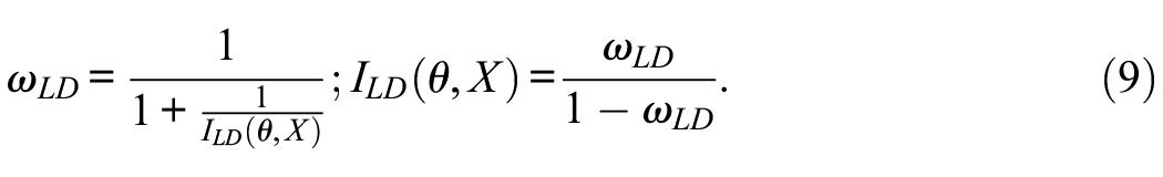
The squared correlation between the sum score and θ as implied by the model in Equation 1 is
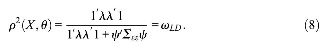
Equation (8) is an expression of the omega reliability coefficient (McDonald, 1985) when correlated residuals exist (Bollen, 1989; Raykov, 2001), which we shall denote here as ωLD. By comparing Equation 7 to Equation 8, the relations between reliability and information under this model are readily found to be
See, for example, the work of Nicewander (1993) for related results. In IRT models in which the score accuracy is expected to vary as a function of θ, reliability and information are alternative and complementary measures of score accuracy (Mellenbergh, 1996; Nicewander, 1993). However, in the linear FA model we are discussing here, neither the reliability nor the information depends on θ. So, their conditional and marginal expressions coincide, and each of them is a one-to-one function of the other. In principle, this relation highlights the alternative interpretations of the measure (Equation 7) we advanced earlier.
Essentially, the information measure in Equations 7 and 9 is a signal/noise ratio (Cronbach & Gleser, 1964) that goes from 0 to infinity, which indicates how many times the common variance of the trait levels in the population is larger than the error variance. Alternatively, Wright (1996) interpreted this type of measure as a “separation ratio” that assesses the extent to which respondents can be effectively differentiated on the basis (in our case) of their sum scores.
Since the reliability and information measures in Equation 9 are one-to-one functions of each other, they might be considered to be redundant. However, as we show below, they each provide an interpretation that complements the other (e.g., Ferrando et al., 2019). In particular, as we shall see, the key point is that the information measure has no upper bound. Therefore, it is far more informative at higher levels of accuracy than a reliability coefficient that is constrained by a unit upper bound (Ferrando et al., 2019; Nicewander, 1993).
Let us now predict the amount of information and reliability that can be attained if the items that are calibrated are locally independent. These predictions are readily obtained by using an identity matrix instead of
Simulation studies that assess the impact of correlated residuals on internal-consistency reliability estimates generally find that these estimates are positively biased, as expected (e.g., Bell et al., 2024; S. B. Green & Hershberger, 2000; Gu et al., 2013). However, in our view, the amount of bias in the accuracy and effectiveness estimates is greater than the reliability-based results suggest. As an example, we shall consider a small simulation dataset we used that was based on a 10-item scale and contained two strong doublets. The correct omega value and the predicted omega under local independence were ω LD = 0.85 and ω LI = 0.90, a difference which seems to be nontrivial but not very large. In terms of information, however, and for the reason discussed earlier, things are different: I LD and I LI were 5.67 and 9, respectively, a considerable difference.
Consider now the ratio
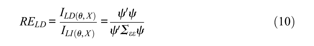
Equation (10) is a relative efficiency measure in the sense discussed by Lord (1980). In our case, it quantifies the change (generally loss) in information that is due to the local dependencies among items. Continuing with our small example provided above, the RE LD is 0.63 which means that the information in the dataset that contains two doublets is only 63% of the information that could be attained if all the items were locally independent.
So far, we have dealt with indices concerned with the first, total score level. We shall now move on to focus on the bivariate level, for which our proposal is simply to use the relative efficiency measure (Equation 10) with each pair of items identified as salient doublets. At this level, Equation 10 reduces, in scalar form, to
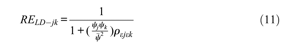
where
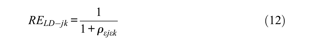
This simplified result enables us to provide some rough initial guidelines. Thus, if the residual correlation is unity, then the doublet relative efficiency is 0.50, which means that the information contributed by the pair is the same as that contributed by a single item. In turn, this result suggests that one of the members can be safely omitted without any loss in accuracy. In contrast, values closer to 1 involve very little or no redundancy, so it is worthwhile to maintain both items even though they have some degree of local dependency.
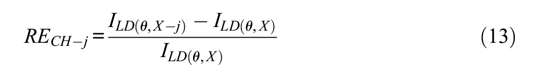
We turn finally to assessment at the single-item level. The standard measure used in this type of assessment is some estimate of the score reliability (generally alpha) if the item were to be deleted (Raykov, 2008; Raykov & Marcoulides, 2011). For a start, what we propose here is to use ω LD to estimate the reliability of the deletion and then complement this index with a relative measure of information change (generally information loss) if the item is deleted. Using the widespread -j terminology, the measure we propose is:
As discussed in the study by Raykov (2008) and Raykov and Marcoulides (2011), blind use of the “reliability estimates if the item is deleted” is not the best choice for “cleaning” a measure and arriving at a final version with the best-possible properties. We agree with this and consider that practitioners have to use these indices critically and make informed choices based on the model-implied properties of the solution. Thus, in the case of a type given in Equation 4 standard solution that fits well, the most likely candidates for deletion are the items with the weakest signal/noise ratio (i.e., low loadings and/or high error variances). In the extended model (Equation 3), however, things become more complex: The candidates are now items which (a) have low signal/noise ratios and/or (b) share a fair amount of specificity with other items in the set and so contribute very little information beyond that provided by the other items (Ferrando & Morales-Vives, 2023). As shown below, the combined use of the indices we propose above when based on informed judgments is particularly effective for item selection.
Indices Based on Nonlinear UVA-FA Solutions
The principles of the UVA (e.g., B. Muthén, 1984) can be directly applied to the type of solution considered here. First, for each item, it is assumed that there is an underlying, continuous-unbounded “strength” latent variable that generates the observed item categorical score. Second, the UVs are related to θ according to the model in Equations 1–3. The UVs are further assumed to be normally distributed with zero mean and unit variance, and the distribution of the residuals εs is also assumed to be multivariate normal with correlation matrix
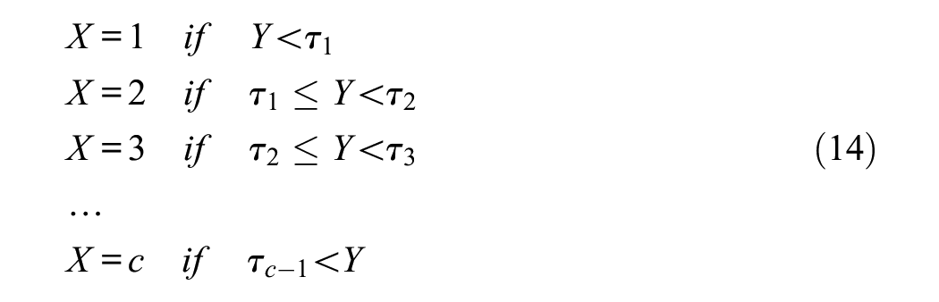
For a response format with c categories, the observed responses are scored with integer values 1, 2 …c. The process that produces the observed categorical scores from the UVs is assumed to be a step function governed by c-1 arbitrary thresholds (τ)
At this point, we should mention the scaling of the structural solution (Equation 3). Because the UV scores are standardized, the inter-item covariance matrix,
The indices we proposed above for the linear case were all obtained from the structural estimates of a solution of the type given in Equation 3. So, it would be straightforward to obtain now their categorical counterparts from the corresponding UVA structural estimates, and in fact, related indices of this type have been proposed as “ordinal” versions of the linear indices (e.g., Zumbo et al., 2007). This type of index, however, reflects the properties not of the sum scores but of the hypothetical sum scores that would be obtained as the sum of the UVs if they were available (see, e.g., Viladrich et al., 2017). We believe that ordinal indices of this type have some interest as upper bounds, but we prefer to derive our indices for the observed sum scores (see Yang & Green, 2015 for a related proposal).
To derive the UVA counterparts of the indices we proposed for the linear model, we shall use the ωLD coefficient as a basis and derive the UVA version of this index by following two requirements. First, it must be defined as the squared correlation between the observed sum scores and θ, as it was in the linear case. Second, it must be obtained from the structural estimates of the UVA solution (i.e., not empirical but model-implied). Thus, the starting expression we wish to estimate is:
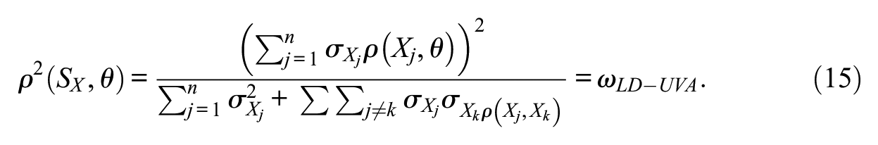
The required model-implied quantities in Equation 14 are obtained as follows. First, the UVA model-implied item means and variances are:

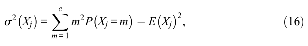
where the Ps are the corresponding areas under the standard normal curve delimited by the thresholds in Equation 13.
The model-implied correlation between each UV and θ (i.e., ρ[Yj,θ]) is indeed the standardized loading λ j and also the polyserial correlation between the manifest item score X j and θ (see Ferrando & Lorenzo-Seva, 2021). Now, the ρ(Xj,θ) correlation in the numerator of Equation 14 is the corresponding point-polyserial correlation. By using the relation between both coefficients (e.g., Olsson et al., 1982, Equation 12), we obtain:
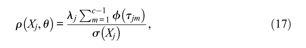
where ϕ is the density of the standard normal distribution. Finally, the model-implied correlation term in the denominator of Equation 14 is obtained as follows. The correlation between the UVs Y j and Y k is (see Equation 3)

And it is also the polychoric correlation between X j and X k . The corresponding product-moment correlation in the denominator of Equation 14 is obtained as
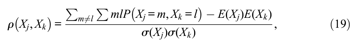
where the Ps are now the threshold-delimited areas in the c×c contingency table obtained using the standard bivariate normal distribution with the correlation value given by Equation 17.
Unlike what occurs in the linear model, in the present model, both the reliability and the information generally vary as a function of θ. Therefore, the reliability coefficient proposed in Equation 14 can be viewed as an estimate (presumably quite close) of the marginal reliability that would be obtained by averaging the conditional score reliabilities across all levels of θ (B. F. Green et al., 1984). The corresponding marginal or average information, denoted here as ILD-UVA, is then obtained by using the relations (e.g., Nicewander, 1993)
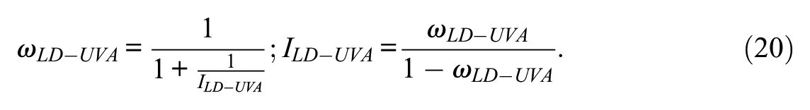
These relations can be interpreted as the inverse of the average squared standard errors of measurement if the sum scores are used for estimating θ and if the UVA solution is correct.
The predicted marginal reliability and information if the items were locally independent will be denoted as ωLI-UVA and ILI-UVA. They are obtained in the same way as ωLD-UVA and ILD-UVA but with all the residual correlations in Equation 17 set to zero. Once the four basic indices have been obtained, obtaining the remaining indices proposed in the previous section is straightforward. Thus, the relative efficiency ratio is obtained as
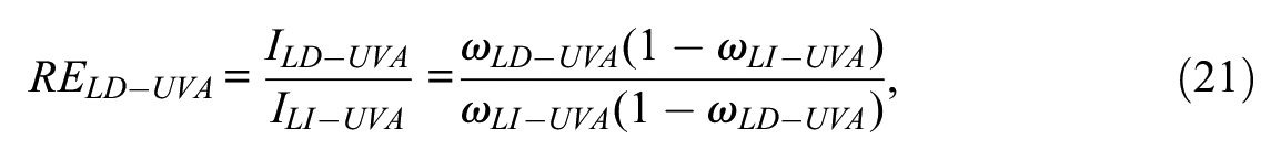
and can be computed at the total score level and at the bivariate-doublet level, as proposed earlier. Finally, the deletion indices on the item-by-item basis can be obtained from ωLD-UVA and ILD-UVA in the same way as explained earlier.
Taking Sampling Error Into Account: CIs
CIs for indices of the type proposed here can be obtained through a variety of procedures, which are both analytical and based on simulation/resampling (e.g., Padilla & Divers, 2016; Raykov & Marcoulides, 2011). Here, we shall propose a simple approach that takes into account the way in which we have implemented our general proposal. So, we expect users to (a) have fitted a structural FA solution with correlated residuals using a program of their choice and then to (b) use the appropriate outcomes to provide the required item structural estimates (i.e., loadings, residual variances/standard deviations, residual correlations, and, in the UVA case, thresholds) as input for obtaining the measures we propose here. We do not expect users to provide the standard errors of the calibration estimates in general, only the point estimates, which initially discourages the use of analytical methods. Furthermore, we assume that the calibration has been based on a reasonably large sample (fitting correlated-residual solutions in small samples is asking for trouble) and that the solution fits acceptably well and can be trusted to be essentially correct. Now, in these conditions, what we propose is to use simulation to obtain percentile CIs. In more detail, users are only asked to provide the structural point estimates together with the size of the sample in which they have been obtained. Next, this solution is taken to be correct and used to generate pseudo-samples or replicas of the same size as that specified by users. Finally, for all the indices of interest, the upper and lower limits of the 90% CIs are taken to be the 5th and the 95th percentile of the distribution across replicas (95% CIs can also be obtained at the request of the user).
The procedure proposed earlier is essentially a modified (not naïve) simulation procedure, expected to produce correct CIs if, as we assume, the null hypothesis that the generating FA solution is correct holds (e.g., Bollen & Stine, 1992). Admittedly, this is a very simple procedure, and further developments can be considered in the future. However, in all the preliminary tests we carried out, it worked very well. Thus, for the reliability estimates in particular, the CIs behaved as can be expected from the theory, and they became narrower as the sample size, number of items, and strength of the solution increased.
Implementation: The Program SINRELEF-LD
The proposal discussed so far has been implemented in an R package called SINRELEF.LD (Score Information, Reliability, & Relative Efficiency under Local Dependences). SINRELEF.LD has been developed in R Version 4.0.2 and runs with R versions more recent than 3.5.0. As input, it uses the calibration item estimates obtained from fitting extended unidimensional FA solutions, which include the existing local dependences. All the implemented procedures can be obtained from linear FA solutions in which the items are treated as approximately continuous or nonlinear solutions in which the item scores are treated as ordered categorical.
The R package includes only one main function, also called SINRELEF.LD, where users have to provide the required inputs to implement the aforementioned procedures.
The uploaded version contains a detailed user’s guide in addition to the documentation already embedded in the R package. Finally, the CRAN upload also has an example dataset that contains some of the data used in the empirical example below.
The SINRELEF.LD package can be downloaded from the CRAN repository at https://cran.r-project.org/web/packages/SINRELEF.LD/index.html.
Empirical Example
For the empirical example, we have used the data of the 928 participants in the study by Dueñas et al. (2022) on the Spanish adaptation of the Family Involvement Questionnaire-High School Version (FIQ-HS). This questionnaire assesses the degree of parental family involvement in the education of their sons and daughters. We have used here only the data on the 17 items of the Home-based activities subscale, which are rated on a 4-point Likert-type scale (rarely, sometimes, often, and always). This subscale includes items on parental activities outside school that promote learning, such as talking with teenage children about careers and schooling and helping them with homework. Previous analyses of the FIQ-HS suggested that the error terms of four pairs of items from this subscale were substantially correlated, which could be explained by the fact that the corresponding item stems either tapped similar content or were very similarly worded.
Based on the nonlinear UVA FA model, a unidimensional solution in which the four doublets referred to earlier were freely estimated was fitted to these data by using robust ULS estimation as implemented in Mplus 8.10 (L. K. Muthén & Muthén, 2017). Goodness-of-fit results were acceptable: RMSEA = 0.057, 90% CI [0.052, 0.063]; Comparative Fit Index (CFI) = 0.91; Goodness of Fit Index (GFI) = 0.95.
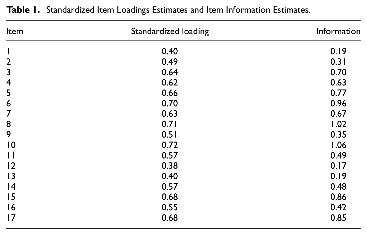
The first step was to inspect the quality of the individual items (reliability and information) when assessed separately. For each item, Table 1 shows the standardized loading estimates (which are item reliability indices) and the item information estimates (which are signal/noise indices as in Equation 9). Because the structural solution that includes the doublet fits well and is essentially correct, these estimates correctly indicate the “a priori” quality of the items. Note that Items 1, 12, and 13 have information values lower than 0.20. The loadings, which range from 0.38 to 0.40, are also the lowest. Therefore, these results suggest that the three items are the ones that function most poorly within the subscale. On the other hand, items 8 and 10 have very high information estimates, both above 1 (i.e., more signal than noise), and the highest loading estimates, both above 0.70.
Standardized Item Loadings Estimates and Item Information Estimates
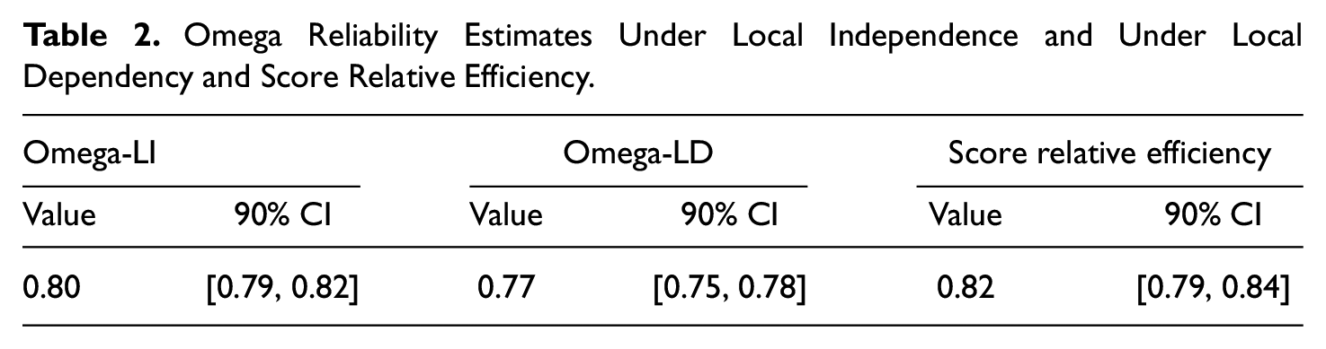
In the second step, the correct omega reliability estimate in which the local dependencies are taken into account (Omega-LD) and the “ceiling” estimate if the items were locally independent (Omega-LI) were obtained and compared (see Table 2). As expected, the value of Omega-LD is the lowest. And although both omega estimates are relatively similar, the CIs do not overlap, and the Omega-LD estimate does not include the 0.80 value commonly considered as a minimum threshold (e.g., Raykov & Marcoulides, 2011). In spite of this, at first glance, it may appear that the loss in reliability due to the related specificities is not large. However, the relative efficiency score in Table 2 suggests that there is an 18% loss of information/efficiency due to the local dependencies modeled in the scale. This is by no means a negligible loss.
Omega Reliability Estimates Under Local Independence and Under Local Dependency and Score Relative Efficiency
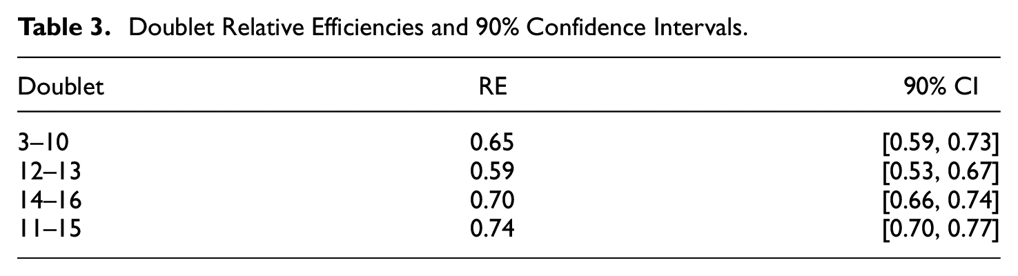
The third step focuses on the bivariate level and consists of inspecting the relative efficiencies of the four salient doublets. The estimates ranged between 0.59 and 0.74 (see Table 3). Because a value of 0.50 means that the pair provides the same information as a single item, values close to 0.50 indicate high redundancy, while values close to 1 indicate very little or no redundancy. In the absence of established cutoff points, we have decided to use 0.70 in this example because, at this value, each item still provides some information that the other item does not. Using this cutoff, we consider that two doublets are especially salient: the pairs 3–10 and 12–13, which are the ones we will discuss in the next step.
Doublet Relative Efficiencies and 90% Confidence Intervals
The fourth step focuses on the single-item level and involves deleting one item at a time and inspecting the results. Table 4 shows the Omega-LD reliability estimates after each item is deleted and the corresponding relative information change. These results may help to decide which items (if any) should be removed from the subscale. However, to grasp the full picture, it is also important to take into account the results obtained in the previous steps and jointly consider (a) the relative efficiency of the doublets (which depends on the magnitude of the doublet and also on the error variance of the items), (b) the signal/noise ratio of each individual item, and (c) the predicted information loss when the item is deleted. Thus, for example, the pair of items 12–13 has the lowest doublet relative efficiency, and both items also have very low information estimates when considered separately (see Table 1). The reason for this last result may be that they both assess content that is peripheral within the construct assessed by this subscale. While most items focus on home activities that are directly related to school or academic progress, these two focus on home activities themselves (Item 12: My teenager has chores to do at home; Item 13: I teach my teenager how to perform home-living skills [ex. laundry, dishes, car maintenance]). There is no doubt that chores at home help teenagers to learn to take responsibility and therefore they have educational value. But the fact that they are not specifically related to school activities makes them somewhat different from the other items. As both items are the same in this respect, and both contribute with low amounts of information, it is only to be expected that deleting one item or the other would not lead to substantially different results. As can be seen in Table 4, both the Omega-LD and the change in relative information are the same if Item 12 or Item 13 is removed. Therefore, in our opinion, there is no compelling rationale for choosing one or the other for deletion.
Omega Reliability Estimates Under Local Dependency After Deleting Each Item, and the Relative Information Change
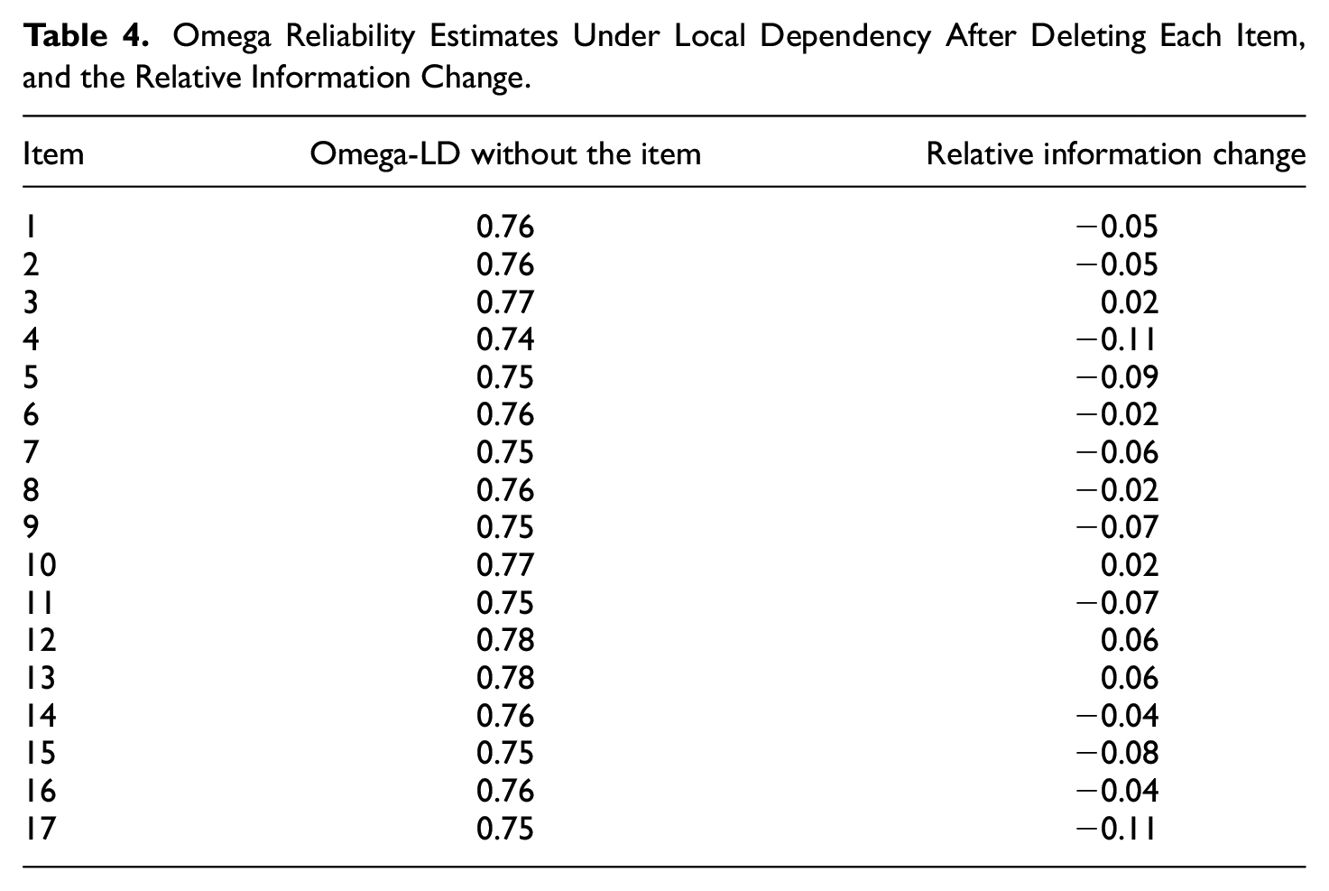
As far as the doublet 3-10 is concerned, the wording of the two items is almost the same (3. I make sure that my teenager has a way to get to school in the morning; 10. I make sure that my teenager has a way to get to home from school in the afternoon), but the estimated amount of information for Item 10 is considerably higher when it is analyzed separately (Table 1). It should be taken into account that this questionnaire assesses the implication of parents in the education of their teenage children. It may be easier for parents to see that their children get to school in the morning (e.g., by taking them on their way to work) than to see that they get home in the afternoon, which may be more difficult to organize and thus say more about their parental involvement. As can be seen in Table 4, removing Item 3 or 10 provides similar Omega-LD estimations and relative information changes, but we consider that it would be preferable to remove Item 3 because the relative efficiency of Item 10 is higher.
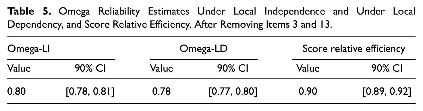
Taking all the above into account, we decided to remove one item from each doublet: Items 3 and 13. Table 5 shows the total score Omega-LD and the Omega-LI estimates, as well as the relative efficiency of the trimmed scale after both items had been removed. As before, the value of Omega-LD is lower than the value of Omega-LI, but now the CIs of these estimations do overlap, and the CI of Omega-LD includes the 0.80 value. The relative efficiency score is now considerably higher than before, having risen from 0.82 to 0.90. Therefore, the loss of information/efficiency due to the modeled local dependences in the scale is now only 10%. In other words, the removal of two items has reduced the redundancies in this subscale and resulted in the Omega-LD value being closer to the Omega-LI value, taking into account the overlapping CIs, and the loss of information/efficiency being reduced. The comparison of the results for the set of 17 items to those for the set of 15 items shows the distortion that the doublets cause in the Omega-LI coefficient and the loss of information/efficiency, which suggests that the Omega-LI coefficient should be interpreted with caution in the presence of doublets and redundant items.
Omega Reliability Estimates Under Local Independence and Under Local Dependency, and Score Relative Efficiency, After Removing Items 3 and 13
Discussion
Many noncognitive measurement instruments contain LIDs, especially when they measure narrow-bandwidth traits. One example is the Satisfaction with Life Scale by Diener et al. (1985), which assesses the narrow-bandwidth variable “satisfaction with life.” In other words, it assesses a highly specific variable, with very few differentiated facets, which, as Ferrando and Morales-Vives (2023) point out, makes the questionnaire redundant even though it is short. In principle, at the calibration or structural level, this problem can be addressed by fitting extended FA solutions that incorporate correlated residuals. If properly used, these solutions are expected to provide (a) correct goodness of model-data fit results, (b) unbiased estimates of the item parameters, and (c) additional information regarding the magnitude and strength of the local dependencies (Ferrando et al., 2024; Mulaik, 2010). The greater flexibility and advantages of an extended solution of this type, however, comes at a cost as it is less parsimonious and potentially more unstable and prone to capitalization on chance than a locally independent solution with a diagonal residual covariance matrix.
At the scoring level, the presence of LIDs in a unidimensional scale is not expected to produce bias (or rather, additional bias) in the derived raw scores when these scores are taken as estimates of the common factor measured (e.g., Yen, 1993). However, they will generally be less accurate and informative than they would be if the items were fully locally independent. So, if the accuracy and information that these scores provide are estimated by assuming full local independence, the reliability and information estimates will be “inflated,” and if there are many dependencies or they are strong, this inflation will be considerable (e.g., Sireci et al., 1991; Wainer & Thissen, 1996). Therefore, the consequences of this incorrect assessment may be far from trivial. To start with, in the stages of test development, the items selected to form the final version of the scale will not be optimal (redundant items will appear to be better than they really are). On the other hand, for existing scales, decisions on individual assessments or score comparisons could be incorrect, as the errors of measurement may be assumed to be smaller than they really are (see Wainer & Thissen, 1996 for a detailed discussion).
The starting point of the present proposal is to use the additional information provided by a structural solution with correlated residuals to correctly assess the “real” quality and accuracy of the scores. This assessment is based on both reliability and information estimates. We then go on to (a) assess the reliability and information that could be attained if the set of items under scrutiny were locally independent and (b) use the results of this assessment as a benchmark for deriving measures of relative efficiency and information loss. These relative measures are derived at three levels: total score, bivariate-doublet, and single-item deletion. Overall, we should point out that everything we propose has been derived for both linear and nonlinear solutions, so the proposal is quite comprehensive.
Admittedly, the assessment we propose will not lead to “complacent” results, as the quality and accuracy estimates are generally deflated, more so when based on information indicators. This result clearly clashes with the widespread practice of reporting score accuracy estimates that are as high as possible (Ferrando & Morales-Vives, 2023; Sabers et al., 1988). In the long term, however, what we propose is expected to result in best practices in both individual assessment and in item analysis and test development. As for the first goal, we believe it is important to correctly assess the accuracy of the scores derived from a scale, since this assessment will indicate the real possibilities of the scores when it comes, for example, to obtaining CIs or establishing cutoff points.
As far as scale development is concerned, the process of selecting the “best” set of items that will form the final version of a noncognitive measure requires trade-offs to attain different and sometimes opposing goals, such as test purpose, simplicity and robustness, brevity, score accuracy, content coverage, and validity. In this process, LIDs may be more or less desirable. So, the recommendation to avoid doublets at all costs mentioned earlier is clearly too simplistic, and our proposal aims to provide more elaborate recommendations. Thus, the doublet relative efficiency measure we propose enables practitioners to take informed decisions on whether to maintain the doublet or split it up given that the two items provide similar information. The empirical example we provide clearly illustrates that the proposal has possibilities.
Finally, one of the strengths of the present study is that all the procedures we propose are implemented as a resource in a free, noncommercial R package that includes a detailed user’s guide and part of the dataset used in the empirical example.
Turning now to limitations and further developments, we expect our proposal to be particularly useful in the specific scenario discussed here: that is, noncognitive measures (personality and attitude), which are analyzed using (linear and nonlinear) FA procedures, and sum scores used as estimates of the individual trait levels. However, other approaches have been proposed in the literature to deal with the issue of local dependencies, and the best-known among them is probably the Testlet Response Theory (TRT; Sireci et al., 1991; Wainer & Thissen, 1996; Wang & Wilson, 2005). Essentially, TRT is an IRT-based approach in which the excess of variation within a bundle of locally dependent items is captured by adding an extra parameter to the IRT model chosen. In the testlet scenario discussed at the beginning of this article in which (a) the testlets are part of the test design (so items can be univocally assigned to testlets), and (b) focus is not on sum scores but on latent trait estimates (generally Bayes estimates), TRT is a strong and powerful approach for calibrating items and for obtaining unbiased estimates of the individual trait levels and accompanying accuracy indicators. This scenario, however, is very different from the one considered here, in which (a) local dependencies are mostly due to faulty test design—and so far less structured—and items cannot be univocally allocated to particular doublets (it is quite usual for an item to appear in several doublets); and (b) one of the issues of interest is to decide which locally dependent items are to be kept and which deleted in order to optimize scale functioning and stability.
Let us now move on to the more specific limitations of what is proposed here. First, much more evidence is needed if we are to decide how to use the indices and to establish cutoffs and reference values. Also, thought needs to be given to developing more complex procedures for obtaining CIs around the proposed indices. In our view, the most immediate developments should focus on the accuracy of the scores derived from the nonlinear UVA solution. The measures we propose are marginal and can be regarded as indicators of the average reliability and information the scores provide across trait levels. So, conditional measures of reliability, information, and relative efficiency across different score levels (e.g., Sabers et al., 1988) would be a welcome complement to what has been proposed here.
Footnotes
Declaration of Conflicting Interests
The authors declared no potential conflicts of interest with respect to the research, authorship, and/or publication of this article.
Funding
The authors disclosed receipt of the following financial support for the research, authorship, and/or publication of this article: This work was supported by the Spanish Ministry of Science and Innovation under grant PID2020-112894GB-I00 and by the Catalan Ministry of Universities, Research and the Information Society under the grant 2021 SGR 00036. The funding source was not involved in any step of the research process, neither in the writing and publication process.