
Abstract
Coefficient omega indices are model-based composite reliability estimates that have become increasingly popular. A coefficient omega index estimates how reliably an observed composite score measures a target construct as represented by a factor in a factor-analysis model; as such, the accuracy of omega estimates is likely to depend on correct model specification. The current paper presents a simulation study to investigate the performance of omega-unidimensional (based on the parameters of a one-factor model) and omega-hierarchical (based on a bifactor model) under correct and incorrect model misspecification for high and low reliability composites and different scale lengths. Our results show that coefficient omega estimates are unbiased when calculated from the parameter estimates of a properly specified model. However, omega-unidimensional produced positively biased estimates when the population model was characterized by unmodeled error correlations or multidimensionality, whereas omega-hierarchical was only slightly biased when the population model was either a one-factor model with correlated errors or a higher-order model. These biases were higher when population reliability was lower and increased with scale length. Researchers should carefully evaluate the feasibility of a one-factor model before estimating and reporting omega-unidimensional.
Keywords
A reliability estimate known as coefficient omega represents the proportion of variance in a composite score (calculated by summing or averaging item scores) explained by a latent variable, or factor, that is common to all items comprising the composite (McDonald, 1999; Zinbarg et al., 2006). Omega estimates have become more popular, largely due to a sizable literature advocating for the use of omega for reliability estimation instead of coefficient alpha (e.g., Dunn et al., 2013; Graham, 2006; McNeish, 2018; Watkins, 2017). Although this literature describes the untenability of essential tau-equivalence and independent errors underlying coefficient alpha, another concern is researchers’ tendency to equate the classical test theory (CTT) true score with a construct score. As Borsboom (2005) and Borsboom & Mellenbergh (2002) have explained, the expected value definition of the CTT true score does not imply that true scores are determined by a single systematic source of variance (i.e., a single construct or latent variable; also see Bollen, 1989; Ellis, 2021). Consequently, although coefficient alpha may remain viable as an estimate of true score reliability (e.g., Raykov & Marcoulides, 2017; Savalei & Reise, 2019; Sijtsma & Pfadt, 2021), it is often an inadequate estimate of the extent to which an observed score is a reliable estimate of a particular construct score, especially for multidimensional composites (Green & Yang, 2015; Reise et al., 2010). Instead, as a reliability estimate based on the common factor model, a coefficient omega index can directly represent the proportion of observed score variance due to a single factor intended to represent a well-defined construct, over and above nuisance variance sources due to extraneous factors or error covariance. For this reason, McDonald (1999) and Zinbarg et al. (2006) claimed that omega is useful as a “construct validity coefficient” in addition to providing reliability information.
It is extremely common for researchers to attempt to estimate the reliability of a composite’s total score under the implied assumption that there is a single construct that all items in the composite have in common (i.e., there is a factor that influences all items; see Flake et al., 2017); a coefficient omega index is meant to do just that. Yet, the term coefficient omega does not refer to a single, specific reliability index. Instead, coefficient omega broadly refers to a set of model-based indices which differ according to the measurement model fitted to the items and how the target construct—the construct that the composite is intended to measure—is represented as a latent variable within that model. In the current paper, we examine the estimates of different omega parameters that are each intended to represent the reliability of a composite score as a measure of a target construct that influences all items; this target construct may be represented by the only factor in a one-factor model, the general factor in a bifactor model, or the higher-order factor in a higher-order model. The methodological literature cited herein commonly defines omega indices with respect to the parameters of these models; consequently, any investigation of the finite-sample properties of omega estimates must draw on these population model structures. Adapting terms from previous sources (e.g., McDonald, 1999; Zinbarg et al., 2006), Flora (2020) refers to these versions of coefficient omega as ωu (i.e., omega-unidimensional), ω H (i.e., omega-hierarchical), and ω ho (omega-higher-order), respectively; we define population parameters for these versions of omega below. Coefficient omega indices not addressed in the current paper include omega-total (representing the proportion of composite variance explained by all factors in the measurement model; Revelle & Zinbarg, 2009) and omega-subscale (also referred to as omega hierarchical subscale, representing the proportion of subscale variance explained by the corresponding specific factor of a bifactor model; Rodriguez et al., 2016).
Coefficient Omega Definitions
First, define xij as the observed score on item j for individual test taker i. Then, the test total score (or composite score) Xi for individual i is simply the sum of the item scores,
Omega-Unidimensional
In its original form, coefficient omega (McDonald, 1999) is a reliability estimate based on the CTT congeneric model (also see Jöreskog, 1971). The congeneric model for the item scores can be expressed as a one-factor model with

where

where
A CFA approach to the estimation of ωu allows the specification of non-zero covariances among the item errors, which in turn impacts the model-implied
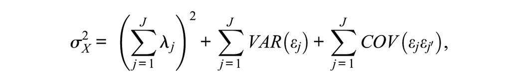
if VAR(f) = 1 as above. If the error covariances are fixed to 0, as is often the case, then the model-implied composite score variance reduces to

which is a common formula for
Furthermore, composite unidimensionality is a strong assumption for ωu. If a one-factor model is not the true data-generating model for the item scores, then fitting a one-factor model to sample data will likely produce ωu estimates that are inaccurate representations of composite reliability with respect to the measurement of a factor that influences all items despite the presence of population-level multidimensionality (hence the motivation for ωH, defined below). In the current study, we investigate the effect of misspecifying a one-factor model for a multidimensional composite, as well as the effect of ignoring true error covariances when estimating ωu with a one-factor model.
Kelley and Pornprasertmanit (2016) suggest that ωu estimates are robust to model misspecification when
Omega-Hierarchical
Tests designed to measure a single target construct often have a multidimensional structure. This multidimensionality is often intentional, as when a test is designed to produce subscale scores in addition to a total score. In other situations, the breadth of the construct definition or aspects of item formats (e.g., wording effects) can produce unintended multidimensionality, even if a general target construct that influences all items is still present. In these situations, the one-factor model is unlikely to explain the item-level data adequately, implying that ωu is an inappropriate measure of how reliably the total score from a multidimensional test measures the target construct.
A bifactor measurement model is often advocated for representing multidimensionality within composite intended to measure a single, general construct (e.g., Rodriguez et al., 2016; Zinbarg et al., 2006). The bifactor model for item score xij can be written as

where gi is the score for individual i on a general factor g that influences all items in the composite and ski is the score on the specific factor k that influences item j. Whereas the general factor loadings λjg are freely estimated for all J items in the composite, each specific factor (also known as a group factor) influences only a subset of items such that factor loadings λjk for specific factor k are freely estimated for a predetermined subset of items (e.g., items within a proposed subscale) and fixed to 0 for all other items. For model identification, the general and specific factors are orthogonal (Yung et al., 1999) and the variance of each factor is fixed to 1.
A version of coefficient omega known as omega-hierarchical, or ωH, is a function of the parameters of a bifactor model fitted to the items comprising a composite and represents the proportion of composite score variance that can be attributed to the general factor (Rodriguez et al., 2016; Zinbarg et al., 2006):

Thus, the formula for ωH is nearly the same as that for ωu, except now the numerator is a function of the general factor loadings. Furthermore, the denominator again represents the composite score total variance which can be estimated from either the model-implied total variance or the observed variance of X. The bifactor model-implied total variance is a function of the general factor loadings, specific factor loadings, and the item error variances (and potential error covariances).
Given our earlier comment that omega-unidimensional (ωu) is likely to be an inaccurate measure of reliability with respect to the measurement of a single factor influencing all items in a multidimensional composite or a unidimensional composite characterized by (ignored) error covariance, the current study also investigates the accuracy of omega-hierarchical (ωH) estimates when the data-generating population model is a bifactor model (correct model specification for ωH), a one-factor model with population-level error covariances (a misspecified model for ωH), or a higher-order model (another misspecified model for ωH); despite differing factor structures, each of these population models is still characterized by having a factor that influences all items. Next, we define omega-higher-order to obtain a correct population omega for the higher-order factor structure against which to compare ωH estimates obtained by fitting a misspecified bifactor model to data from a higher-order population model.
Omega-Higher Order
Although ωH is often recommended as a reliability estimate for the measurement of a target construct influencing all items in a multidimensional composite (e.g., Green & Yang, 2015; Reise et al., 2013; Watkins, 2017), the bifactor model underlying ωH may not be the correct population model structure for a target construct influencing all items. Alternatively, researchers may hypothesize a higher-order factor structure such that a broad, overarching latent variable (a higher-order factor) causes individual differences in several more conceptually narrow lower-order factors, which in turn directly influence the observed item responses. This model can be expressed with

where fki is an individual’s score on lower-order factor k; each lower-order factor influences only a subset of items, such that factor loadings λjk for lower-order factor k are freely estimated for a subset of items (e.g., items within a proposed subscale) and fixed to 0 for all remaining items. Then, instead of allowing the lower-order factors to freely covary with each other, each is directly regressed on a higher-order factor:

where hi is the score on the higher-order factor, γk is the higher-order factor loading for the kth lower-order factor, and ζk is an error term. This higher-order model is identified if there are at least three lower-order factors (Rindskopf & Rose, 1988).
Omega-higher order, or ωho, is a function of the parameters of a higher-order model fitted to the items comprising a composite and represents the proportion of composite score variance that can be attributed to the higher-order factor. Because the associations between the higher-order factor and the observed item scores are mediated through the lower-order factors, ωho is a function of these indirect effects; each indirect effect of the higher-order factor on an item score is the product of the item’s lower-order factor loading and the corresponding higher-order factor loading (i.e., λjk*γk; Raykov & Zinbarg, 2011). Consequently,

with the numerator of ωho equaling the squared total of the indirect effects of the higher-order factor on the observed item scores and the denominator again representing the variance of the composite score. 3
Although the bifactor model and the higher-order model are formally related (see Yung et al., 1999), the bifactor model’s general factor and a higher-order factor have different interpretations: The bifactor general factor has direct effects on the item scores with the effects of the specific factors covaried out, whereas the higher-order factor has indirect effects on the item scores which act entirely through the lower-order factors. Yet, a higher-order factor and a bifactor model’s general factor are both latent variables that influence all items in a multidimensional composite and therefore estimates of ωH may provide reasonable approximations to ωho. Another aim of the current study is to assess this possibility.
The Current Study
The purpose of each version of coefficient omega presented above is to quantify the proportion of composite score variance due to a latent variable that influences all items comprising the composite, with ωu being a function of the parameters of a one-factor model, ωH based on the parameters of a bifactor model, and ωho based on the parameters of a higher-order model. In practice, the true measurement model for a set of items is unknowable, and researchers must rely on a variety of model fit statistics, comparisons of competing models, and previous evidence to support their hypothesized measurement model. Yet, researchers often estimate the reliability of a composite without first testing its dimensionality, which in turn can lead to misleading estimates using either coefficient alpha or ωu as researchers may often assume that the composite score is a measure of a target construct that influences all items (see Flake et al., 2017). This practice may be indirectly encouraged by recent resources that facilitate the calculation of ωu without the explicit estimation of a factor analysis model (Hancock & An, 2020; Hayes & Coutts, 2020; Kelley, 2022; Pfadt, van den Bergh, Sijtsma, Moshagen, & Wagenmakers, 2022); these implementations return omega estimates which are implicitly based on a one-factor model (estimates of ωu) with uncorrelated error terms, regardless of whether that model adequately represents the data.
Alternatively, other resources (Gignac, 2014; Green & Yang, 2015; Reise et al., 2013; Rodriguez et al., 2016; Watkins, 2017) advocate estimating the reliability of a multidimensional composite score with respect to the measurement of a general factor common to all items; that is, ωH, by fitting a bifactor model to item-level scores. Yet, other work has cautioned against the overuse of bifactor models (e.g., Bonifay et al., 2017; Markon, 2019; Reise et al., 2016). Simulations have shown that a bifactor model can produce as good or better fit statistics than the correct model when fit to data from unidimensional, two-factor, and higher-order populations (e.g., Maydeu-Olivares & Coffman, 2006; Morgan et al., 2015; Murray & Johnson, 2013); Bonifay and Cai (2017) found that even when data were generated to follow random patterns, the bifactor model had good fit to a high percentage of samples.
Therefore, it is possible that researchers will report an omega estimate based on an incorrect measurement model and consequently reach an inaccurate conclusion about composite reliability. That is, the true proportion of composite score variance due to a target construct that influences all items may be best defined by a one-factor model (with or without error correlations), a bifactor model, or higher-order model, whereas researchers may be likely to estimate this proportion using an omega estimate calculated from a misspecified model. As yet, the degree to which different coefficient omega statistics differ from the proportion of composite variance due to a target construct when the model is incorrectly specified is not fully known, as previous studies on this issue are limited. Therefore, the main purpose of the current study is to investigate the impact of major model misspecification on the accuracy of ωu and ωH estimates as measures of the proportion of composite score variance due to a factor influencing all items. In practice, however, it may be that major model misspecification would be detected by common model fit statistics (e.g., root mean square error of approximation [RMSEA], comparative fit index [CFI]), thus leading researchers to revise a hypothesized model (e.g., by freeing error correlation parameters) and then calculate a more accurate omega estimate from the parameter estimates of the revised model. Hence, a secondary purpose of the current study is to investigate the associations between the accuracy of omega estimates and popular model fit statistics.
Previous studies have found that omega estimates are generally unbiased under correct model specification (e.g., Yang & Green, 2010; Zinbarg et al., 2006). Zinbarg et al. (2006) simulated data from a higher-order population model and found that ωH produced relatively unbiased estimates of the proportion of variance explained by the higher-order factor, especially with higher values of population ωho and longer composites; however, this study did not include ωu estimates and used a very low number of replications. Yang and Green (2010) found that ignoring non-zero error covariances led to positively biased estimates of ωu, although the relative bias was only around 5% with six-item composites and decreased to approximately 2% with a 12-item composite. Yang and Green also simulated data from a bifactor model, but compared ωu estimates from a misspecified unidimensional model with a population analog of omega-total (i.e., the proportion of composite variance due to both general and specific factors) rather than ωH. In the current study, we are instead interested in comparing ωu estimates with population ωH to determine how well ωu estimates the proportion of variance explained by a single factor that is common to all items despite population-level multidimensionality.
To address the issues described above, the current paper presents a Monte Carlo simulation study of the finite sample properties of coefficient omega estimates of the proportion of composite score variance due to a single factor that influences all items as a function of correct and incorrect model specification. Specifically, this study investigated the following research questions:
Our study further considers the effects of the composite length (i.e., number of items), magnitude of population omega, and sample size. We expected that omega estimates calculated from a correctly specified measurement model would be unbiased, but that unmodeled complexity (i.e., incorrectly fitting a unidimensional model to a multidimensional test or incorrectly fixing all error covariances to zero) would introduce considerable bias for ωu estimates of the proportion of variance due to a factor common to all items. Furthermore, we expected that ωH estimates would provide reasonably accurate estimates of the proportion of variance due to a factor common to all items even when the true model is not a bifactor model (e.g., a higher-order factor model).
Method
To investigate our research questions about ωu and ωH estimates, a series of Monte Carlo simulations were run using the SimDesign package in R (Chalmers & Adkins, 2020; R Core Team, 2020); all simulation code is publicly posted at https://osf.io/k7jtz/. Sample data were drawn from multivariate normal distributions with covariance structures consistent with given population CFA models using the mvrnorm function of the MASS package (Venables & Ripley, 2002). Models were estimated using the maximum likelihood estimator in the lavaan package (Rosseel, 2012) and ωu and ωH were estimated using semTools (Jorgensen et al., 2020). The proportion of total score variance due to the factor common to all items, which we refer to as population reliability from here forward, was calculated for each population model and compared with sample omega estimates for 1,000 random samples for each cell of the study design. When non-converged or improper model solutions were obtained for a given cell of the study design, additional replications were drawn until the total number of converged replications with proper solutions equalled 1,000. In total, there were four population factor structures and both a high and low reliability model were generated for both long and short composites. Each factor model was estimated with three sample sizes, creating a total of (4 × 2 × 2 × 3) = 48 unique cells.
Study Conditions
Sample data were generated from four population models: a simple one-factor model with no correlated errors, a one-factor model with correlated errors, a bifactor model, and a higher-order model; path diagrams of these models are in Figures 1 through 4. All models were specified such that factor variances equaled 1.0; consequently, the population-level model-implied covariance structures were in the correlation metric. Samples generated from the simple one-factor model were fit only to the correct model across replications. For samples drawn from all other population models, a simple one-factor model, a correlated errors one-factor model, and a bifactor model were fit to the sample data. Therefore, data from the correlated one-factor and bifactor population models were fit to a correctly specified model as well as two incorrectly specified models, while data from the higher-order populations were fit only to incorrectly specified models.
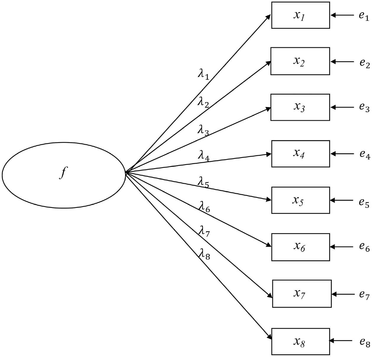
Simple One-Factor Population Model.
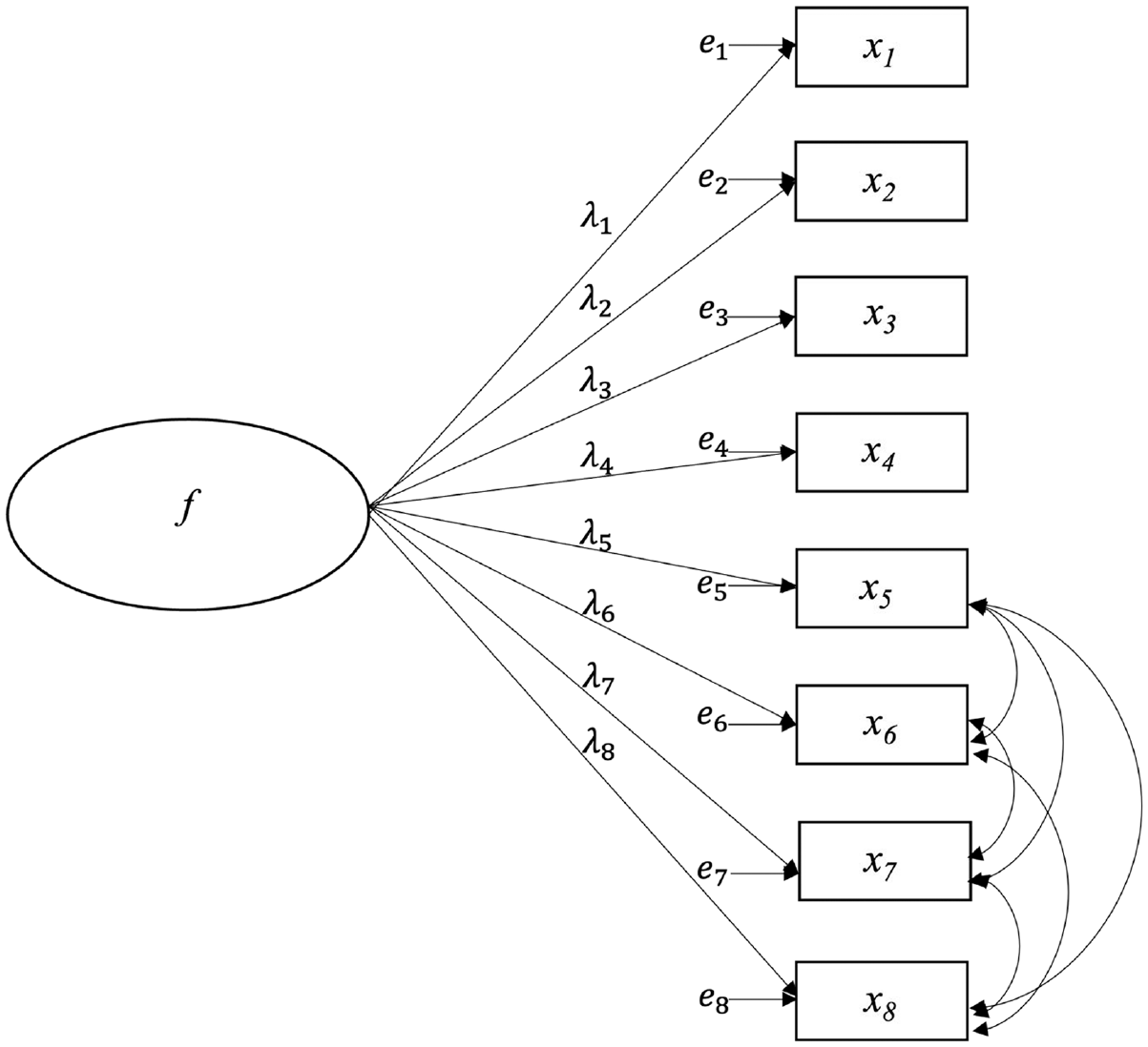
One-Factor Population Model With Correlated Errors.
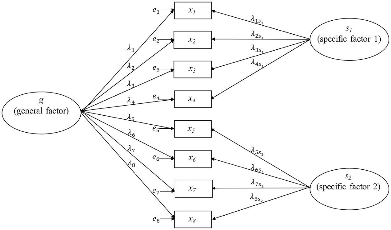
Bifactor Population Model.
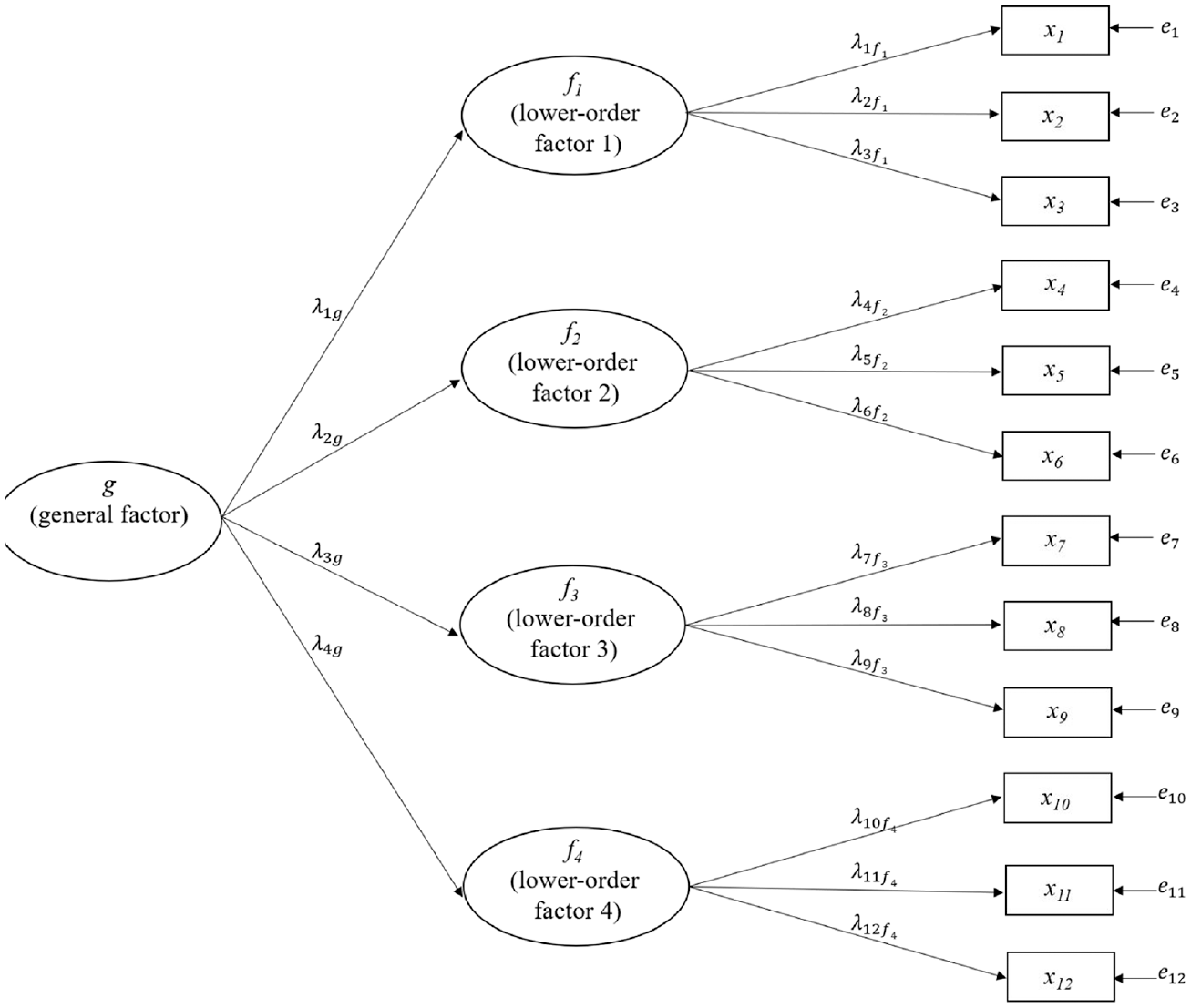
Higher-Order Population Model.
For each population model structure, there were two conditions of population reliability (i.e., population omega) determined as a function of factor loading parameters. The high-reliability condition set population reliability to .85 while population reliability was .60 in the low-reliability condition. Scale lengths were either short (8 items) or long (16 items) except for the higher-order model, where scale lengths were necessarily longer to ensure enough indicators per factor for model identification. For the higher-order population condition, the short scale was 12 items (three indicators per lower-order factor) and the long scale was 20 items (five indicators per lower-order factor). We chose these values of population reliability and composite length to be representative of situations commonly encountered in practice, as described by Flake et al. (2017). There were three sample size conditions: N = 100, selected to reflect what is often considered a small sample for the purpose of CFA; N = 250, a medium-sized, commonly observed sample size; and N = 1,000, which is typically considered a large sample for CFA.
Table 1 gives the factor loading parameter values for each model. Factor loadings for the correlated one-factor model ranged from .493 to .837 in the high-reliability conditions and from .493 to .624 in the low-reliability conditions. Half of the item errors for the correlated errors model were allowed to correlate (see Figure 2), as allowing all errors to freely correlate would have produced under-identified models. The error correlations were small to moderate in the high-reliability conditions (approximately .09–.31) and moderate to high in the low-reliability conditions (approximately .19–.52). In a typical bifactor model, every item loads onto both a general factor and a specific factor. However, preliminary simulations showed that bifactor models with two specific factors fitted to data from the one-factor, correlated errors model could not converge consistently. Therefore, only one specific factor capturing these error correlations was included along with the general factor when bifactor models were fitted to data from the one-factor, correlated errors model.
Population Factor Loadings and Error Covariances for Each True Model
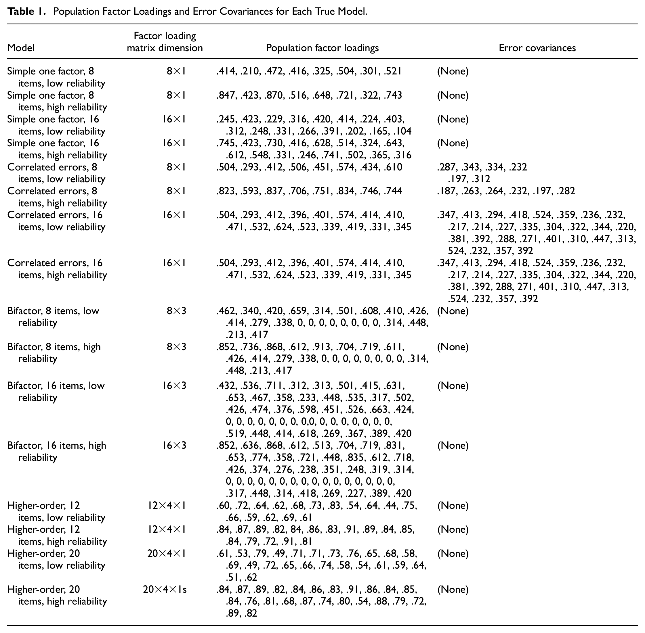
The bifactor population models were specified to include two specific factors pertaining to equal composite halves and a single general factor influencing all items (see Figure 3). The correlated errors model fit to sample data from a bifactor population model allowed all items within each half to correlate with one another, but not with items from the other half of the composite. See Table 1 for population factor loading values across the high- and low-reliability conditions.
Finally, the higher-order population model included a single higher-order factor and four lower-order factors; four is the smallest number of lower-order factors by which a higher-order model can be empirically distinguished from a correlated-factor model (Rindskopf & Rose, 1988). See Table 1 for population factor loading values.
Evaluation of Results
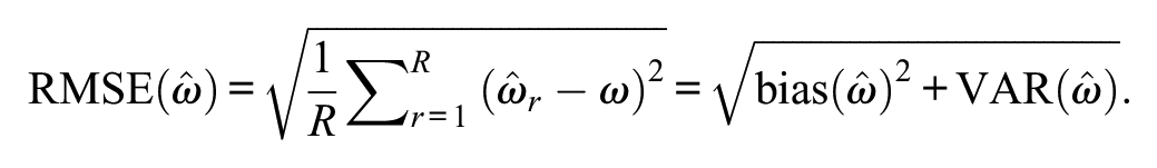
For each replication, ωu and ωH estimates (i.e.,

where R is the number of replications,
We also present side-by-side boxplots of omega estimates across conditions to convey the estimate distributions graphically.
Results
Convergence and Proper Solutions
Table 2 shows the proportions of replications that failed to converge to a proper solution per study condition. In general, estimation of bifactor models was most likely to produce convergence failures, regardless of population model, as bifactor models fitted to data from a bifactor population had the highest error rates. Non-convergence was mitigated by sample size, such that an increase in sample size produced fewer errors for all conditions. The fewest errors occurred when estimating one-factor models with no correlated errors, where only three replications failed to produce proper solutions, all from samples of N = 100.
Proportions of Replications That Failed to Converge With Proper Solutions Per Condition
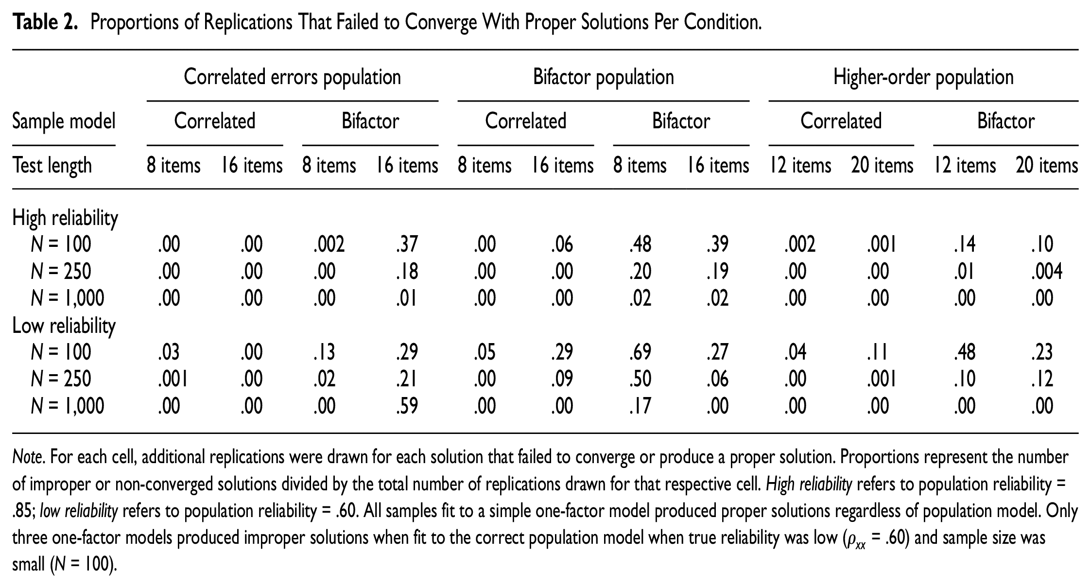
Note. For each cell, additional replications were drawn for each solution that failed to converge or produce a proper solution. Proportions represent the number of improper or non-converged solutions divided by the total number of replications drawn for that respective cell. High reliability refers to population reliability = .85; low reliability refers to population reliability = .60. All samples fit to a simple one-factor model produced proper solutions regardless of population model. Only three one-factor models produced improper solutions when fit to the correct population model when true reliability was low (
Simple One-Factor Population Model
Table 3 shows the mean bias and RMSE of
Mean Bias and RMSE of Omega-Unidimensional Estimates (
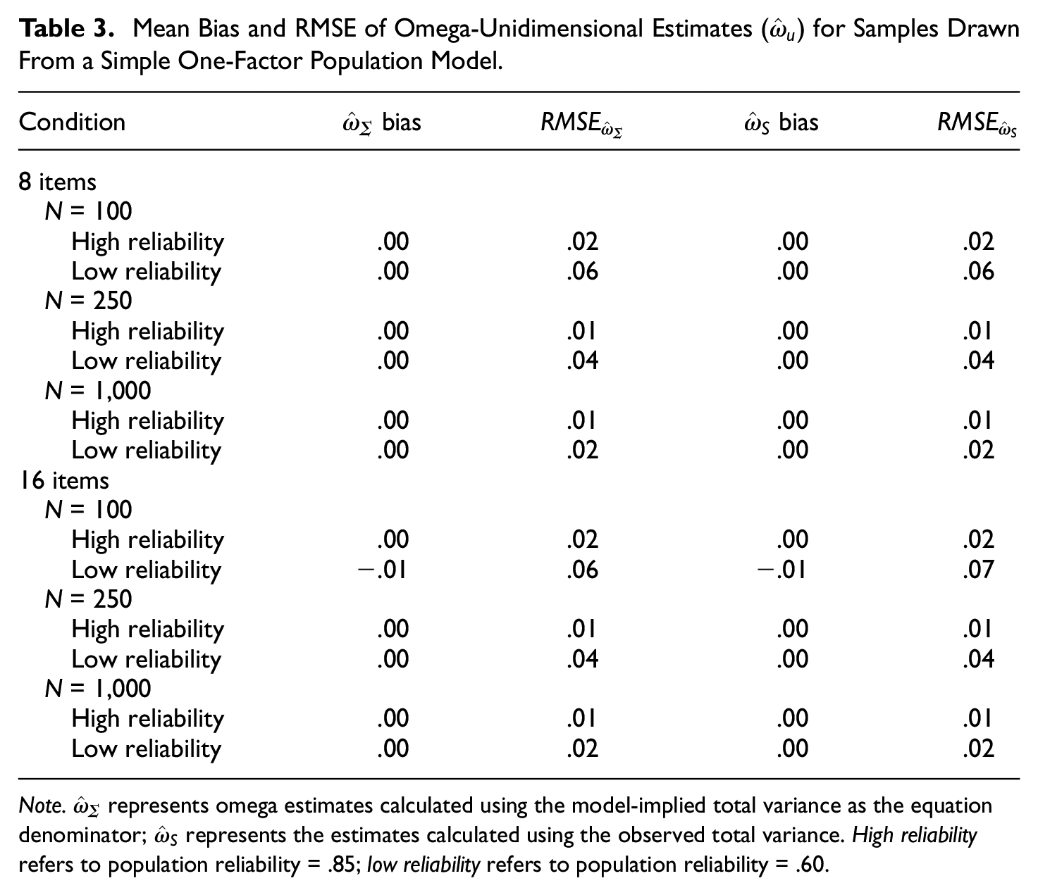
Note.
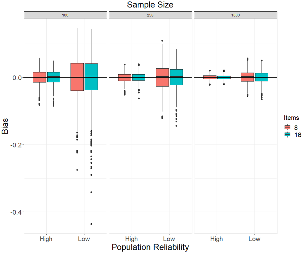
Boxplots of Bias of ωu Estimates (Using the Model-Implied Total Variance as Its Denominator) Obtained in the Population One-Factor Model (No Correlated Errors) Conditions.
One-Factor Population Model With Correlated Errors
The mean bias and RSME for omega estimates from a one-factor population model with correlated errors are shown in Table 4, and the distribution of bias with N = 250 is shown in Figure 6 (similar patterns were observed across sample sizes; see online supplement for figures with N = 100 and N = 1,000). Estimating the correct model yielded unbiased
Mean Bias and RMSE of Omega Estimates for Samples Drawn From a One-Factor Population Model With Correlated Errors
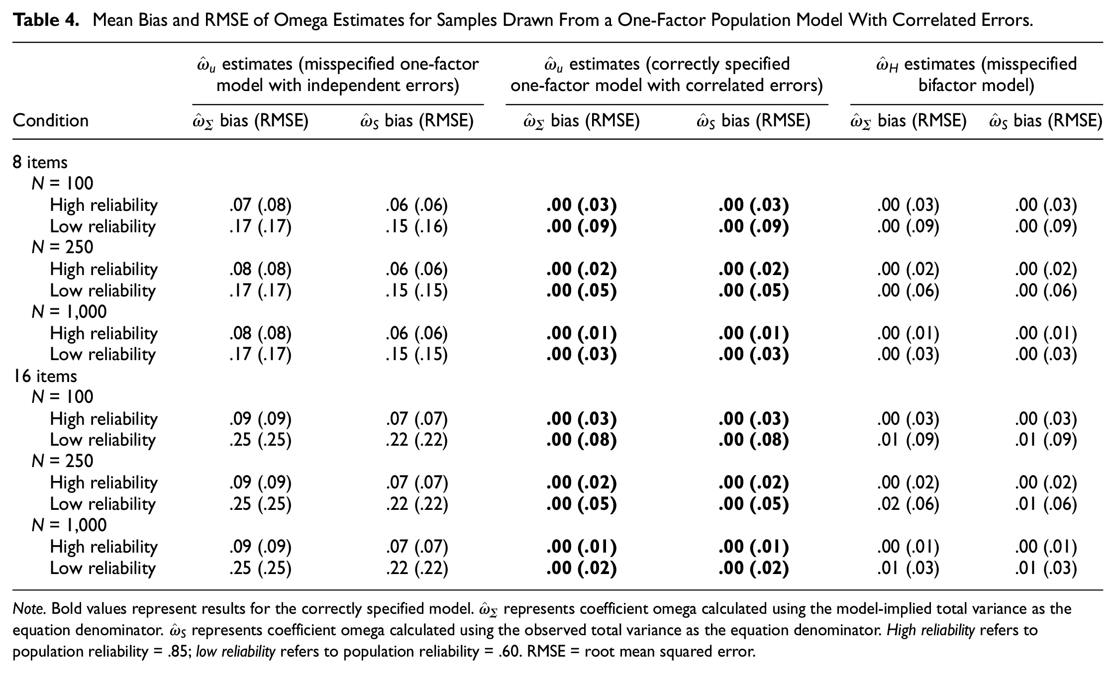
Note. Bold values represent results for the correctly specified model.
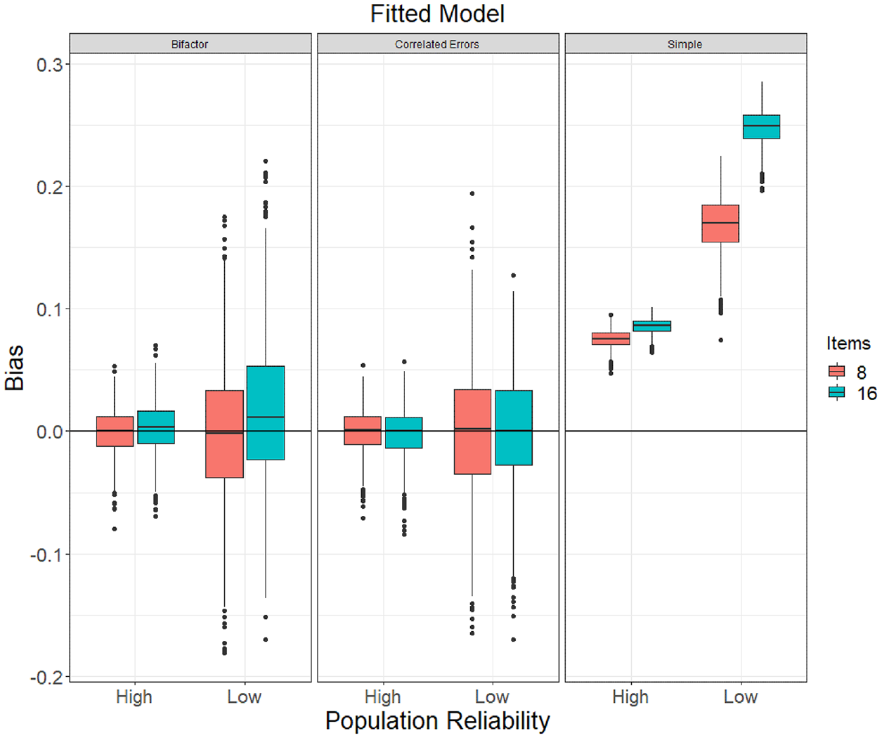
Boxplots of Bias of ω Estimates (Using the Model-Implied Total Variance as its Denominator) by Fitted Model Specification Obtained With Samples of N = 250 Drawn From the Population One-Factor Model, Correlated Error Conditions. Middle Panel Corresponds to the Correct Model Specification Condition. “Simple” Refers to a One-Factor Model With No Error Correlations.
The misspecified, simple one-factor model produced highly biased
Bifactor Population Model
Table 5 shows the mean bias and RMSE of omega estimates from a bifactor population model and Figure 7 shows the distributions of bias with N = 250 (see online supplement for figures with N = 100 and N = 1,000). A correctly specified bifactor model produced relatively unbiased
Mean Bias and RMSE of Omega Estimates for Samples Drawn From a Bifactor Population Model
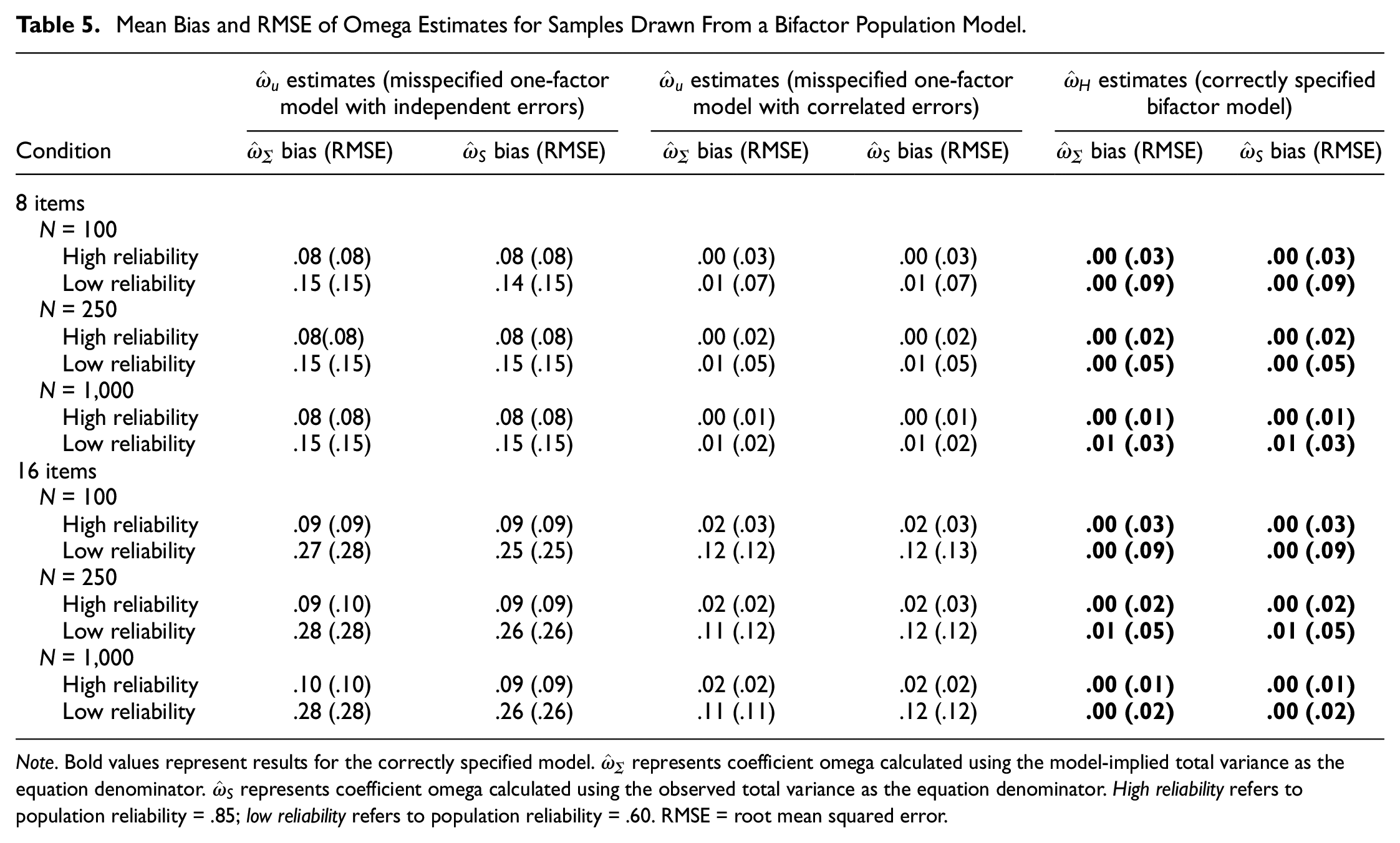
Note. Bold values represent results for the correctly specified model.
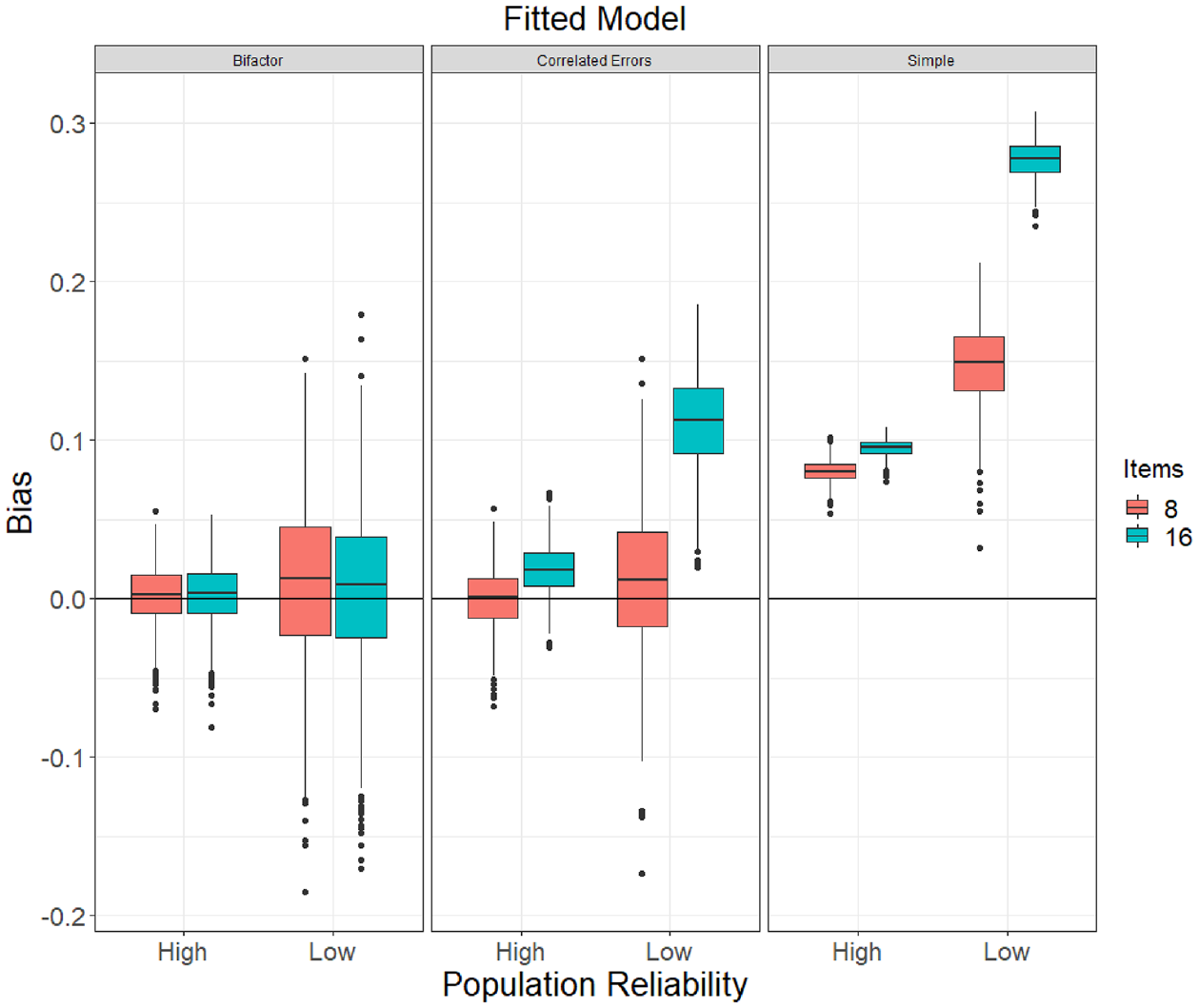
Boxplots of Bias of ω Estimates (Using the Model-Implied Total Variance as Its Denominator) by Fitted Model Specification Obtained With Samples of N = 250 Drawn From the Population Bifactor Model. Left Panel Corresponds to the Correct Model Specification Condition. “Simple” Refers to a One-Factor Model With No Error Correlations.
When
When
Higher-Order Population Model
The bias and RMSE of omega estimates obtained from the higher-order population model are in Table 6, and distributions of bias are shown in Figure 8 (see online supplement for figures with N = 100 and N = 1,000). When
Mean Bias and RMSE of Omega Estimates for Samples Drawn From a Higher-Order Factor Population Model
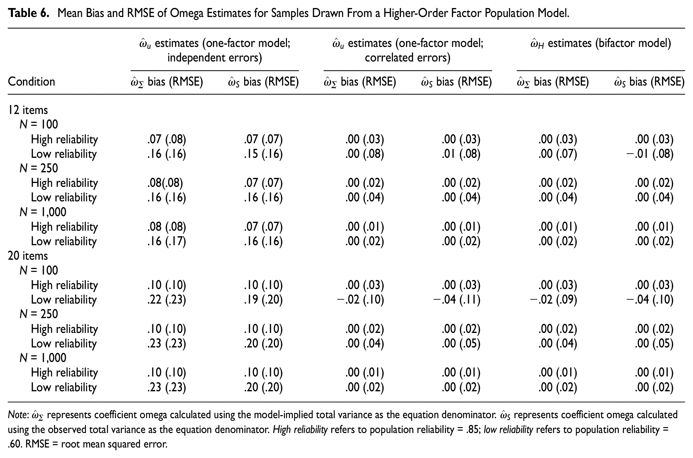
Note:
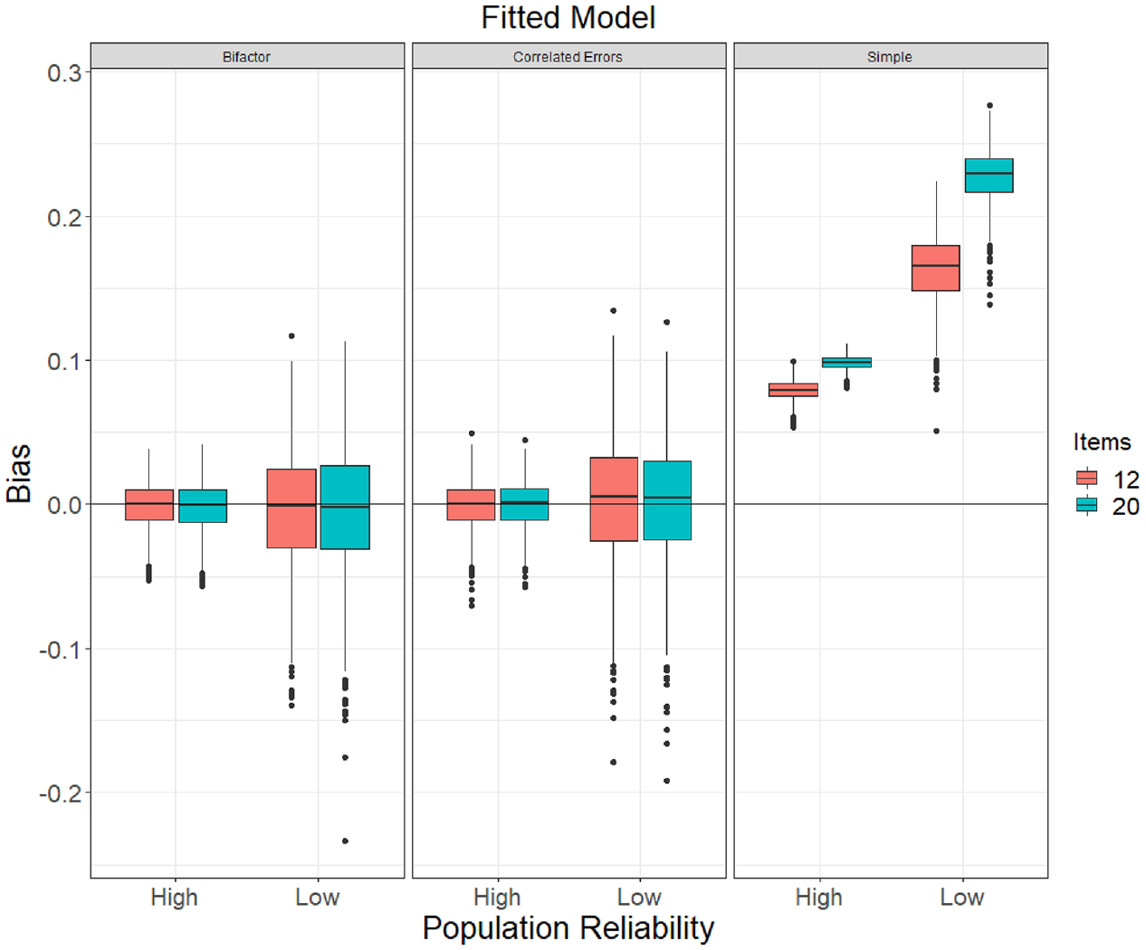
Boxplots of Bias of ω Estimates (Using the Model-Implied Total Variance as Its Denominator) by Fitted Model Specification Obtained With Samples of N = 250 Drawn From the Population Higher-Order Model. “Simple” Refers to a One-Factor Model With No Error Correlations.
Denominators of Coefficient Omega
For all conditions, omega estimates were calculated using both the model-implied total variance of the composite sum score and the observed sum score variance, as explained earlier. In general, there were only small differences in omega estimates between the two calculations. When models were correctly specified, mean bias and RMSE were nearly identical; when omega estimates were obtained from misspecified models, using the observed variance offered a very slight advantage over the model-implied variance, but differences in mean bias did not exceed .03 in any cell of the study and RMSE differences were negligible.
Relationship With Model Fit
We also investigated whether the accuracy of omega estimates corresponded to model fit using three major model fit statistics (RMSEA, CFI, and Tucker–Lewis index [TLI]). Because bias could be positive or negative, lower values did not necessarily indicate lower bias. Therefore, we assessed the relation between the absolute value of bias and model fit, but not direction of bias.
Table 7 shows rank-order correlations between descriptive model fit statistics and absolute values of bias of omega estimates within each population model. In general, results for the CFI and TLI were such that better model fit (higher fit index values) was associated with lower bias. Correlations with CFI and TLI were relatively weak (−.14 or weaker) when the fitted model was correctly specified, and strongest when simple one-factor models were incorrectly fitted to data drawn from more complex population model structures (from −.25 to −.74). Regarding RMSEA, the correlations generally indicated that better fit (lower values of RMSEA) was weakly associated with lower bias, except for strong, negative correlations between RMSEA and bias occurring when simple one-factor models were incorrectly fitted to data from other population structures. Scatterplots of RMSEA by bias revealed strong, non-monotonic patterns, indicating that these negative correlations occurred because of strong negative associations with RMSEA values ranging from approximately .12 and greater, whereas when RMSEA was in a range generally indicative of good to marginal fit (RMSEA < approximately .10), the association between RMSEA and bias was rather flat.
Spearman Correlations Between Bias and Model Fit Indices
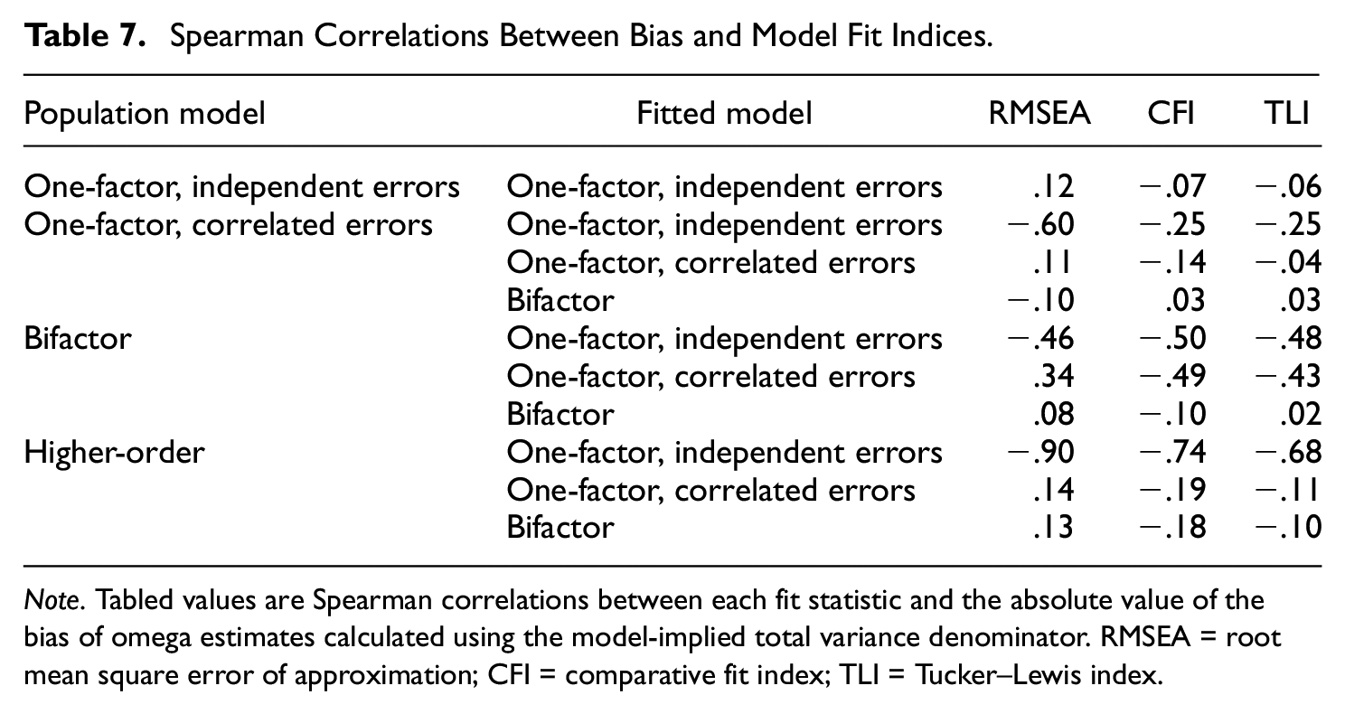
Note. Tabled values are Spearman correlations between each fit statistic and the absolute value of the bias of omega estimates calculated using the model-implied total variance denominator. RMSEA = root mean square error of approximation; CFI = comparative fit index; TLI = Tucker–Lewis index.
Discussion
Coefficient omega has become a popular composite reliability index, as multiple authors have suggested that omega estimates should be broadly preferred over coefficient alpha. Yet, coefficient omega does not refer to a single reliability estimate; instead, alternative versions of omega differ depending on the factor-analytic measurement model fitted to item scores (see Flora, 2020). Specifically, the current paper focuses on omega-unidimensional, ωu, which represents the proportion of total score variance due to the single factor of a one-factor model, and omega-hierarchical, ωH, which represents the proportion of total score variance due to the general factor of a bifactor model. Both ωu and ωH measure the proportion of composite score variance due to a single factor that influences all items; the primary aim of the current study was to determine whether ωu and ωH can provide unbiased estimates of this proportion when the underlying measurement model is misspecified. Our results are consistent with previous studies, which indicate that omega estimates are generally accurate under correct model specification and that misspecification leads to increased bias as population reliability decreases (e.g., Yang & Green, 2010; Zinbarg et al., 2006).
Performance of
u Estimates
Estimates of ωu calculated from a correctly specified one-factor model were unbiased on average, regardless of composite length (8 vs. 16 items) and population reliability (.60 vs .85), and showed good precision given an adequately large sample size (N≥ 250). However,
In our one-factor, correlated errors population condition, the error correlations were rather large, having been chosen to represent a situation where item wording effects, such as those obtained with negatively valanced item stems (i.e., items that would typically be reverse scored), are particularly strong. In many applied situations, however, error correlations among item scores are much weaker (e.g., .10 or less). When population error correlations are in this smaller range, the bias in
Our results support Yang and Green’s (2010) observation that failure to specify true correlated errors for a one-factor model will result in substantial bias for
In conclusion, researchers should report
Performance of
H Estimates
In addition, we assessed how well estimates of ωH, which is based on the parameters of a bifactor model, represent the proportion of composite variance due to a single factor common to all items under conditions of correct and incorrect model specification. Previous simulations have indicated that bifactor models may be overused and can produce good model fit statistics due to overfitting (e.g., Bonifay & Cai, 2017; Morgan et al., 2015). Yet, our results showed that while
The ability of
Observed Versus Model-Implied Variance
In that each version of coefficient omega considered herein is a measure of the proportion of composite score variance explained, another research question for the current study was whether there is any advantage to calculating omega estimates as a function of observed composite variance instead of the model-implied composite variance. Our results provided only modest support to the claim by Kelley and Pornprasertmanit (2016) that use of observed total variance is robust to misspecification in that estimates calculated using observed variance were only slightly less biased than estimates based on model-implied variance in the conditions with the most severe model misspecification; yet, Kelley and Pornprasertmanit only studied minor misspecification in their simulations. Bentler (2009) suggested that use of model-implied composite variance would lead to more efficient omega estimates, but our results do not support this proposal, instead showing that omega estimates based on the observed composite variance have comparable or slightly less variation (as shown by our RMSE values) than estimates computed with the model-implied variance.
Associations With Model Fit
Finally, we also examined the associations between common descriptive model fit statistics—RMSEA, CFI, and TLI—and the bias of omega statistics as estimates of the proportion of composite variance due to a factor influencing all items. If the bias of omega estimates is highly correlated with model fit, then in practice, a researcher may detect model misspecification by observing a high RMSEA or low CFI, revise the hypothesized model (e.g., by freeing error correlation parameters), and then calculate an appropriate omega estimate from the parameter estimates of the revised model and could thereby avoid calculating a highly biased omega estimate altogether. We did find modest correlations between model fit statistics and bias of omega estimates, suggesting some protection against model misspecification, especially when simple one-factor models were fitted to data drawn from more complex models. But there are situations in which misspecified models still fit sample data well, which could lead to researchers obtaining an omega estimate that overestimates how precisely a composite measures a factor common to all items. In addition to model fit statistics, researchers should employ theory, results of CFAs from previous studies, and model comparison (using statistics such as the Bayesian Information Criterion, BIC) to establish the optimal measurement model for a composite prior to calculating an omega estimate.
Implications for Applied Research
The current findings have important implications for researchers wishing to estimate composite reliability using coefficient omega. Here, we remind the reader that applied researchers are often interested in determining how reliably a composite measures a target construct, which can be represented by a factor in a factor-analysis model and does not necessarily correspond to the CTT true score (Borsboom, 2005). In the current study, we investigated how well different forms of coefficient omega estimate the proportion of total composite variance that is due to a factor that influences all items in a composite as a function of model misspecification. In other words, we investigated how well omega estimates the reliability of a composite as a measure of a common factor. The high bias of
Regarding software implementation, we used the reliability function of the semTools package in R to obtain all omega estimates in the current study. This function automates the calculation of omega from the estimates from a CFA model previously fitted using the lavaan package, and as such, the user is required to estimate a measurement model for the composite prior to calling the reliability function, which will subsequently return omega values giving the estimated proportion of composite variance explained by each factor in the CFA model. For this reason, we recommend the general use of semTools::reliability as demonstrated in the Flora (2020) tutorial, as users are forced to consider an appropriate CFA model before obtaining omega estimates. The ci.reliability function of the MBESS package (Kelley, 2022) calculates
A more encouraging result from our study is that
Alternatively, output of the omega function of the popular R package psych (Revelle, 2022) provides a statistic labeled “omega hierarchical” which is calculated by (a) fitting a EFA model (with three factors by default) to the item-level data, (b) rotating the factors obliquely and determining higher-order factor loadings from the inter-factor correlation matrix, (c) applying the Schmid-Leiman transformation to obtain an exploratory bifactor model, and finally (d) calculating an omega index as a function of the resulting general factor loadings. Thus, psych::omega is an attractive option for researchers who determine that a simple unidimensional model is not appropriate for their composite but are not able to specify a theoretically informed CFA model. Nevertheless, we caution that the omega-hierarchical statistic provided by psych::omega does not correspond to the
Limitations and Directions for Future Research
This study investigated the accuracy of omega estimates under a range of conditions; however, as with all simulation studies, there are omitted conditions which should be addressed by future studies. Although correct versus incorrect model specification was the primary independent variable of our design, this manipulation was constrained to selection of an incorrect model type (i.e., one-factor models with and without error correlations, bifactor model, or higher-order model). The effect of more minor misspecification—for example, failing to model cross-loadings or small correlated errors within a bifactor model—was not addressed. Further studies should verify and expand on these findings by examining different types and degrees of misspecification. In addition, although the current study involved generating data from a higher-order population model to compare
Next, we generated data from the multivariate normal distributions implied by our population model specifications. This procedure allowed us to examine the effects of model misspecification (as well as scale length and strength of population omega) without the confound of categorical versus continuous responses. In practice, many composites are comprised of binary or ordered, categorical item response variables which are best modeled with a categorical variable methodology, such as by fitting CFA models to polychoric correlations. In these situations, estimates of coefficient omega should be adapted to enable the CFA model’s estimates to be properly scaled into the composite’s observed total score metric (see Flora, 2020; Green & Yang, 2009b; Yang & Green, 2010). Therefore, important expansions on the current findings will be to investigate the performance of omega estimates for both continuous and categorical item–response variables under additional conditions of misspecification.
Conclusion
Numerous authors have advocated for the regular use of coefficient omega to estimate composite reliability in place of more traditional indices such as coefficient alpha, despite that there is relatively little simulation evidence about the finite sample properties of different forms of coefficient omega. Many of these recommendations focus on omega-unidimensional and pay little heed to its dependence on the adequacy of a one-factor model for item-level data; similarly, omega-hierarchical is based on the parameters of a bifactor model, but it has been shown that misspecified bifactor models often fit item-level data well. The current paper presents a simulation study indicating that omega-unidimensional and omega-hierarchical provide unbiased estimates of the reliability of a composite with respect to the measurement of a target construct when the fitted factor model is correctly specified. However, under misspecification, omega-unidimensional provided strongly biased estimates of the reliability of a composite as a measure of a factor common to all items and should therefore only be used in the case of a single-factor congeneric model, with care taken to account for potential error correlations among items. Omega-hierarchical, however, provided relatively unbiased estimates of composite reliability with respect to a general factor influencing all items, even when the population model was a higher-order model or a one-factor model with correlated errors. Researchers who wish to use estimate reliability using omega should therefore take care to ensure adequate sample size (N≥ 250) and carefully factor analyze their results to select the best model, based not only on fit indices but also on theory and previous evidence.
Footnotes
Declaration of Conflicting Interests
The authors declared no potential conflicts of interest with respect to the research, authorship, and/or publication of this article.
Funding
The authors received no financial support for the research, authorship, and/or publication of this article.