Sage Journals: Discover world-class research

Abstract

A recurring question regarding Likert items is whether the discrete steps that this response format allows represent constant increments along the underlying continuum. This question appears unsolvable because Likert responses carry no direct information to this effect. Yet, any item administered in Likert format can identically be administered with a continuous response format such as a visual analog scale (VAS) in which respondents mark a position along a continuous line. Then, the operating characteristics of the item would manifest under both VAS and Likert formats, although perhaps differently as captured by the continuous response model (CRM) and the graded response model (GRM) in item response theory. This article shows that CRM and GRM item parameters hold a formal relation that is mediated by the form in which the continuous dimension is partitioned into intervals to render the discrete Likert responses. Then, CRM and GRM characterizations of the items in a test administered with VAS and Likert formats allow estimating the boundaries of the partition that renders Likert responses for each item and, thus, the distance between consecutive steps. The validity of this approach is first documented via simulation studies. Subsequently, the same approach is used on public data from three personality scales with 12, eight, and six items, respectively. The results indicate the expected correspondence between VAS and Likert responses and reveal unequal distances between successive pairs of Likert steps that also vary greatly across items. Implications for the scoring of Likert items are discussed.

Keywords

Likert scales visual analog scales item response theory continuous response model graded response model

Most psychometric tests and questionnaires are currently administered with a Likert format in which respondents mark their position along a discrete range with somewhere between four and seven levels of gradation. Depending on the item content, this gradation may represent levels of agreement with a statement, levels of severity of some symptom, or temporal frequency of occurrence of that symptom. Such response levels are regarded as ordinal steps along a presumed continuous dimension and the Likert format is generally preferred over a simpler yes–no format that forces respondents to express only all–or–none positions. Thus, switching from just two (i.e., yes–no) to more response alternatives per item is regarded as allowing for finer granularity that, in turn, might result in more precise measures or more ability to discriminate respondents from one another (see, for example, Alan & Kabasakal, 2020; Donnellan & Rakhshani, 2023; Maydeu-Olivares et al., 2009; Müssig et al., 2022; Shi et al., 2021). In the limit, a continuous response format can be implemented via a visual analog scale (VAS) on which respondents mark any position along a continuous line, limited only by the resolution with which the mark can be made and subsequently read off. This should provide the largest possible precision on the assumption that respondents can actually use this response format consistently and in full, which does not seem to be the case (see, for example, Furukawa et al., 2021; Gideon et al., 2017; Krosnick, 1991; Preston & Colman, 2000).

Digital technology allows administering tests with VAS or Likert formats equally easily (see, for example, Kinley, 2022; Reips & Funke, 2008) and some studies have investigated the classical psychometric properties (i.e., reliability, validity, factor structure, etc.) of the same tests administered under each response format (see, for example, Kuhlmann et al., 2017; Preston & Colman, 2000; Simms et al., 2019). Generally, these studies have not found any evidence that a potentially limited ability of respondents to use the VAS format in full has deleterious effects on those properties but, at the same time, the continuous VAS format does not seem to improve those properties beyond what a discrete Likert format provides.

Then, in principle, psychometric instruments administered with Likert or VAS formats might be considered equivalent as regards their global properties, but it is not immediately obvious that this is the result of analogous response processes on the part of the respondents. Justification for a VAS format arises from consideration that respondents may feel that their position lies somewhere between any two consecutive discrete landmarks in a Likert scale. Then, because the VAS format allows respondents to express their position with higher resolution, a seemingly reasonable surmise is that a Likert response is simply a quantization of the corresponding VAS response. Thus, one may surmise (a) that the VAS continuum is partitioned into a discrete number of exhaustive and mutually exclusive intervals and (b) that the Likert response is that associated with the interval on which the VAS response would had fallen. Analyzing VAS and Likert data produced by a sample of respondents in consecutive administrations of the same test with each format would reveal whether or not this is the case and it could additionally illustrate how the VAS continuum is partitioned, with direct attention to the issue of whether or not the partition involves intervals of the same width within and across items.

Several studies have addressed in various forms the question of whether the steps in a Likert format involve jumps of the same magnitude. For instance, Knutsson et al. (2010) had respondents indicate the perceived magnitude with which they felt that typical category labels on a Likert item express severity of symptoms, frequency of symptoms, or level of agreement. Their results indicated that progressive grading via labels does not map onto constant increases in perceived magnitude. Toland et al. (2021) administered a four-item instrument with the VAS format and subsequently discretized the responses into 10, five, or four discrete categories by partitioning the VAS continuum into intervals of equal size. They argued that if the equal-interval assumption held for the VAS scale, analysis of the discretized responses via polytomous item response theory (IRT) models would render category location parameters that are equispaced. Their results indicated otherwise and they rejected the equal-interval assumption. An analogous approach based on checking for equidistant category threshold parameters in polytomous IRT accounts of Likert data was used by Sideridis et al. (2023) and they concluded that their results ruled out the equal-interval assumption.

The work described in this article addressed this question differently and using publicly available data collected by Kuhlmann et al. (2017) in a study involving dual administration of three personality scales, once with a VAS format and once with a 5-point Likert format. IRT allows obtaining separate characterizations for Likert data via the graded response model (GRM; Samejima, 1969) and for VAS data under the continuous response model (CRM; Samejima, 1973). A comparison of both IRT characterizations reveals the similarities and differences between VAS and Likert response processes, including a quantitative description of how Likert responses may arise from partitioning the VAS continuum into a number of intervals whose boundaries are implicitly indicated by GRM and CRM item parameter estimates. Estimates of these boundaries allow a direct test of the equal-interval assumption.

Theoretical justification for the specific form of our analysis is given in the next section, which shows that CRM item parameters can be transformed into equivalent GRM item parameters under arbitrary assumptions about the discretization process by which continuous (VAS) responses map onto discrete (Likert) responses. This theoretical analysis also indicates how CRM and GRM item parameter estimates should be used to estimate the boundaries of the discretization intervals by which VAS responses are mapped onto Likert responses on each individual item. A simulation study then checks out the accuracy with which these relations hold in finite samples, also looking at the corresponding item and test information functions and at the accuracy of estimation of respondents’ trait levels under each response format. Finally, an analogous analysis conducted on Kuhlmann et al.’s (2017) data reveals characteristics that are compatible with the theoretical and simulation results presented earlier, indicating that VAS and Likert response processes share common features that are not immediately apparent in a simple comparison of raw VAS and Likert data. Estimates of discretization boundaries varied greatly across items and they did not support the equal-interval assumption. In addition, this analysis did not find any sign that a VAS format actually improves the accuracy with which respondents’ trait levels can be estimated. Implications of these results for empirical practice are finally discussed, with emphasis on the limited advisability of the VAS response format as a replacement for the conventional Likert response format.

Formal Relation Between CRM and GRM

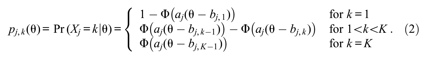
In Samejima’s (1969) normal-ogive graded response model (NO-GRM) for a Likert item with K ordered response categories, the probability $p_{j, k}^{*}$ of observing a response beyond category k (1 ≤k≤K− 1) on item j increases with trait level θ according to

p_{j, k}^{*} (θ) = \Pr (X_{j} > k | θ) = Φ (a_{j} (θ - b_{j, k})),

(1)

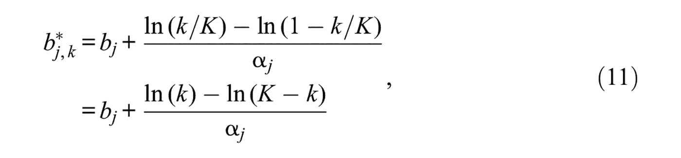
where a_j is the item discrimination parameter, b_j,k is the threshold parameter between categories k and k+ 1, and Φ is the unit-normal cumulative distribution function. Thus, a K-category item is described by K parameters with values varying across items. By subtraction, the category response function (CRF) describing the probability p_j,k of observing a response in category k (1 ≤k≤K) on item j varies with trait level θ according to

p_{j, k} (θ) = \Pr (X_{j} = k | θ) = {\begin{matrix} 1 - Φ (a_{j} (θ - b_{j, 1})) & for k = 1 \\ Φ (a_{j} (θ - b_{j, k - 1})) - Φ (a_{j} (θ - b_{j, k})) & for 1 < k < K \\ Φ (a_{j} (θ - b_{j, K - 1})) & for k = K \end{matrix} .

(2)

Note that the (discrete) response X_ij∈ {1, 2, . . ., K} to item j by the ith respondent with trait level θ_i is a multinomial random variable with parameters (1, p_j,₁(θ_i), p_j,₂(θ_i), . . ., p_j,K(θ_i)).

Samejima (1973, 2005) defined the CRM to be the limiting case of the NO-GRM as the number of categories approaches infinity. Then, the expression in Equation 2 invariably yields p_j,k(θ) = 0 because the response Y_j to item j is a continuous random variable bounded, without loss of generality, in [0, 1]. The CRM posits that Y_j has the conditional distribution (see, for example, Ferrando, 2002; Wang & Zeng, 1998; Zopluoglu, 2013):

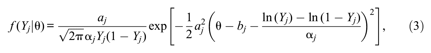
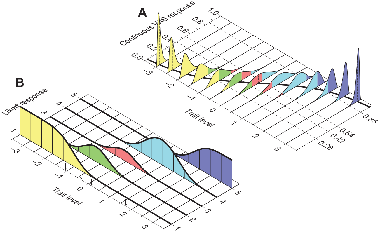
f (Y_{j} | θ) = \frac{a_{j}}{\sqrt{2 π} α_{j} Y_{j} (1 - Y_{j})} \exp [- \frac{1}{2} a_{j}^{2} {(θ - b_{j} - \frac{\ln (Y_{j}) - \ln (1 - Y_{j})}{α_{j}})}^{2}],

(3)

where a_j, b_j, and α_j are item parameters. Despite the putative infinite number of response categories, an item is described under the CRM with fewer parameters than those necessary to describe the same item administered in Likert format with K > 3 response categories. The reason is immediately obvious by inspection of Figure 1, which shows the conditional distributions in Equation 3 at trait levels ranging from −3 to 3 in steps of 0.5 for an item with a = 2, b = 0, and α = 1 (Figure 1A) and an item with a = 4, b = 0.5, and α = 1.8 (Figure 1B). The red sigmoid on the bottom plane depicts the expected item score, that is, how the expected value of Y, E(Y|θ), varies with θ. Item parameter b is the value of θ at which E(Y|θ) = 0.5. On the other hand, item parameters a and α jointly determine the slope of this sigmoidal curve and how the variance of the conditional distribution of Y varies with θ.

Figure 1.

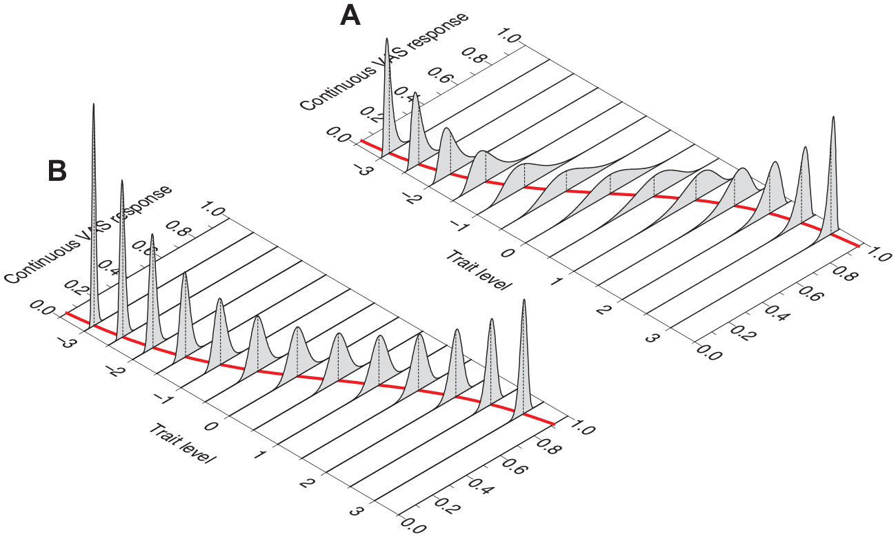
Conditional Distribution of the Continuous VAS Response Y at Several Trait Levels θ (From −3 to 3 in Steps of 0.5). The Red Sigmoid on the Bottom Plane Describes the Expected Item Score as a Function of θ, that is, How the Expected Value of Y Varies with Trait Level. (A) Item Parameters are a = 2, b = 0, and α = 1. (B) Item Parameters are a = 4, b = 0.5, and α = 1.8

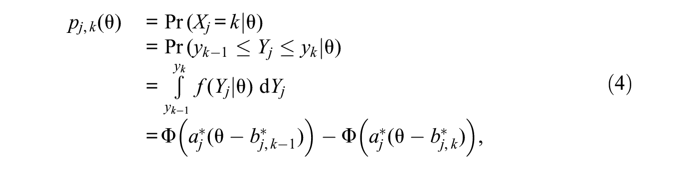
Although NO-GRM and CRM parameterizations appear incommensurate at first glance, a simple relation between them can be formally derived under the assumption that Likert responses arise by quantization of the continuous response dimension. This assumption is often made when VAS responses are discretized into K categories for analysis or for comparison with actual Likert responses (see, for example, Flynn et al., 2004; Toland et al., 2021; van Laerhoven et al., 2004; Vickers, 1999). This approach to discretization partitions the bounded VAS continuum into K exhaustive and mutually exclusive intervals of the same width, with the original VAS response Y placed into the applicable interval to render the Likert response X. More generally, consider a partition of the interval [0, 1] into K regions with arbitrary boundaries y₁, y₂, . . ., y_K₋₁ subject to the order constraint y₀ < y₁ < y₂ < . . . < y_K₋₁ < y_K, with y₀ = 0 and y_K = 1. Then, for 1 ≤k≤K,

\begin{matrix} p_{j, k} (θ) = \Pr (X_{j} = k | θ) \\ = \Pr (y_{k - 1} \leq Y_{j} \leq y_{k} | θ) \\ = \int_{y_{k - 1}}^{y_{k}} f (Y_{j} | θ) d Y_{j} \\ = Φ (a_{j}^{*} (θ - b_{j, k - 1}^{*})) - Φ (a_{j}^{*} (θ - b_{j, k}^{*})), \end{matrix}

(4)

with

a_{j}^{*} = a_{j},

(5)

b_{j, k}^{*} = b_{j} + \frac{\ln (y_{k}) - \ln (1 - y_{k})}{α_{j}} .

(6)

Note that $b_{j, 0}^{*}$ in Equation 6 goes to −∞ and, thus, the right-hand side of Equation 4 reduces to $1 - Φ (a_{j}^{*} (θ - b_{j, 1}^{*}))$ for k = 1; analogously, $b_{j, K}^{*}$ in Equation 6 goes to ∞ and the right-hand side of Equation 4 reduces to $Φ (a_{j}^{*} (θ - b_{j, K - 1}^{*}))$ for k = K. Thus, Equation 4 matches Equation 2, which is the CRF for category k in the NO-GRM for a K-category Likert item. Discretization of continuous responses for an item with CRM parameters a_j, b_j, and α _j thus results in discrete responses conforming to an NO-GRM characterization with item parameters $a_{j}^{*}$ and $b_{j, k}^{*}$ from Equations 5 and 6, for 1 ≤k≤K− 1. This process is illustrated in Figure 2 for a five-category discretization of the item in Figure 1A using boundaries (y₁, y₂, y₃, y₄) = (0.26, 0.42, 0.54, 0.85).

Figure 2.

Transformation of Continuous VAS Responses Into Discrete Likert Responses Over K = 5 Categories for the Item in Figure 1A, With CRM Parameters a = 2, b = 0, and α = 1. Dashed Lines at (y₁, y₂, y₃, y₄) = (0.26, 0.42, 0.54, 0.85) in Panel (A) Indicate How the Continuous VAS Dimension is Partitioned into K = 5 Exhaustive and Mutually Exclusive Intervals. By Equation 4, the Probability of a Response Falling in Each Interval at any Given Trait Level is Given by the Area Under the Corresponding Conditional Distribution of Y Within the Corresponding Interval, Indicated with a Different Color for Each Interval. Panel (B) Plots These Probabilities as a Function of Trait Level, Yielding the Item CRFs Under the NO-GRM. Small Vertical Arrows Along the Trait Level Axis Indicate the Resultant NO-GRM Threshold Parameters via Equation 6, Namely, $(b_{j, 1}^{*}, b_{j, 2}^{*}, b_{j, 3}^{*}, b_{j, 4}^{*}) = (- 1.046, - 0.323, 0.160, 1.735)$

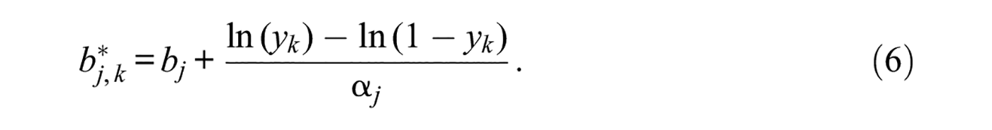
Three aspects of this formal equivalence are worth pointing out. First, the number and locations of the boundaries y_k do not affect the validity of Equation 4 although variations in these locations affect the resultant $b_{j, k}^{*}$ and, thus, the shapes that the CRFs under the NO-GRM characterization can describe for the exact same CRM item. Second, boundary locations may vary across items and, then, they are more appropriately denoted y_j,k. Importantly, the location of these boundaries can be estimated by rearranging Equation 6, that is,

y_{j, k} = \frac{1}{1 + \exp [α_{j} (b_{j} - b_{j, k})]},

(7)

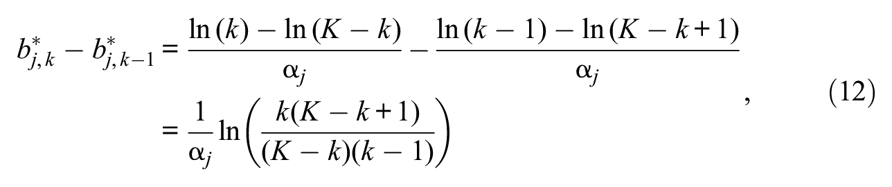
for 1 ≤k≤K− 1. Note that $b_{j, k}^{*}$ in Equation 6 has been replaced with b_j,k in Equation 7 to emphasize the fact that practical use of Equation 7 involves CRM and NO-GRM item parameters independently estimated from VAS and Likert data, respectively, provided by the same sample of respondents. Finally, discretization boundaries for any given item might also vary across respondents, but these variations are much harder to model and virtually impossible to estimate. Strictly speaking, discretization boundaries whose locations vary across respondents are tantamount to item parameters that vary across respondents.

The formal relation in Equation 4 allows expressing the operational characteristics of the same item under both the CRM and the NO-GRM. This, in turn, permits a theoretical comparison of the potential of the two response formats in practical applications, particularly as regards the accuracy of estimation of respondents’ trait levels. In IRT, this is captured by the item information function (IIF). Under the CRM, Samejima (1973) showed that

{IIF}_{j}^{CRM} (θ) = a_{j},

(8)

that is, the IIF is constant and independent of θ. In contrast, the IIF under the NO-GRM is

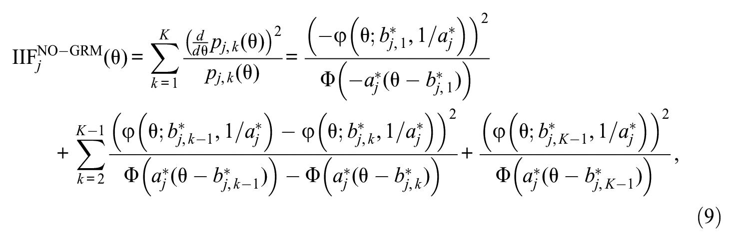
\begin{array}{l} {IIF}_{j}^{NO-GRM} (θ) = \sum_{k = 1}^{K} \frac{{(\frac{d}{d θ} p_{j, k} (θ))}^{2}}{p_{j, k} (θ)} \\ = \frac{{(- φ (θ; b_{j, 1}^{*}, 1 / a_{j}^{*}))}^{2}}{Φ (- a_{j}^{*} (θ - b_{j, 1}^{*}))} + \sum_{k = 2}^{K - 1} \frac{{(φ (θ; b_{j, k - 1}^{*}, 1 / a_{j}^{*}) - φ (θ; b_{j, k}^{*}, 1 / a_{j}^{*}))}^{2}}{Φ (a_{j}^{*} (θ - b_{j, k - 1}^{*})) - Φ (a_{j}^{*} (θ - b_{j, k}^{*}))} + \frac{{(φ (θ; b_{j, K - 1}^{*}, 1 / a_{j}^{*}))}^{2}}{Φ (a_{j}^{*} (θ - b_{j, K - 1}^{*}))}, \end{array}

(9)

with item parameters from Equations 5 and 6, and where $φ (θ; μ, σ)$ denotes the probability density function of a normally-distributed random variable with mean μ and standard deviation σ. Figure 3 shows the IIFs for the two CRM items in Figure 1 and their corresponding NO-GRM versions obtained with discretization boundaries (y₁, y₂, y₃, y₄) = (0.26, 0.42, 0.54, 0.85) (red curves) or with a uniform partition into intervals of identical width via (y₁, y₂, y₃, y₄) = (0.2, 0.4, 0.6, 0.8) (blue curves). At least for these two sample items, the Likert response format seems superior in the central range of trait levels and the continuous response format only seems superior at extreme trait levels. These differences may have important implications for trait estimation that will be assessed in subsequent sections of this article. On the other hand, equispaced boundary locations for discretization of the response continuum results in Likert items with symmetric IIFs centered on the value of the CRM parameter b.

Figure 3.

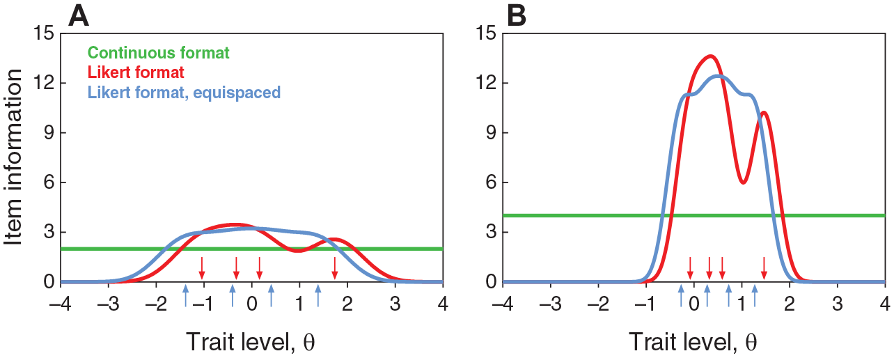
Item Information Functions for the Items in Figures 1A (Left Panel) and 1B (Right Panel) Under the Continuous Response Format (Green Horizontal Lines), the Likert Response Format After Discretization With (y₁, y₂, y₃, y₄) = (0.26, 0.42, 0.54, 0.85) (Red Curves), and the Likert Response Format After Discretization With (y₁, y₂, y₃, y₄) = (0.2, 0.4, 0.6, 0.8). Colored Arrows Along the Horizontal Axis in Each Panel Indicate the Location of the NO-GRM Category Threshold Parameters $b_{j, k}^{*}$ That Result From Each Type of Discretization of Each Item

Simulation Study

This proof-of-concept simulation assesses the feasibility of a quest for common processes underlying VAS responding and Likert responding in finite samples. Initial data sets were generated by simulating continuous responses to CRM items; Likert responses were created either by discretization of continuous responses with arbitrary boundaries or by independent simulation of responses to equivalent NO-GRM items. Estimates of item parameters and respondents’ trait levels were obtained from CRM and NO-GRM data sets and compared according to the theoretical relations presented earlier. Results are presented in detail for the main (and representative) simulation run; results for other runs are summarized at the end of this section.

Data Generation

The simulation run described here in detail involved a 15-item test and 10,000 respondents. True trait levels were randomly drawn from a unit-normal distribution. For direct comparison with estimates of trait levels (see below) the resultant values were rescaled to zero mean and unit standard deviation. True CRM item parameters were randomly drawn from uniform distributions in the range [1.5, 2.5] for a, [−1.2, 1.2] for b, and [1, 2] for α. This strategy intentionally avoids Shojima’s (2005) decision to keep in a simulation the ratio of a to α at unity for each item and the average b across items at zero.

Continuous responses Y_ij in the range [0, 1] were generated by randomly drawing deviates from the conditional distributions in Equation 3, using the ith respondent’s trait level and the jth item parameters for each Y_ij. For this purpose, normal deviates z_ij with mean $α_{j} (θ_{i} - b_{j})$ and standard deviation $α_{j} / a_{j}$ were first obtained, subsequently converted into Y_ij via

Y_{ij} = \frac{\exp (z_{ij})}{1 + \exp (z_{ij})},

(10)

and finally rounded to three decimal places.

Likert responses X_ij were obtained in two ways. The first one was by discretization of the continuous responses just generated, using boundaries (y₁, y₂, y₃, y₄) = (0.2, 0.4, 0.6, 0.8). Likert responses obtained in this way are completely determined by continuous responses. A separate strategy disengaged Likert from continuous responses as follows. First, matching NO-GRM item parameters were obtained from true CRM item parameters via Equations 5 and 6. Then, NO-GRM Likert responses were generated with X_ij as a realization of a multinomial random variable with the distribution in Equation 2, using the same respondents’ trait levels that had been used for the generation of continuous responses.

Other simulation runs were analogous and involved different numbers of items, different numbers of respondents, and different discretization boundaries that were fixed for all items or that varied randomly across items.

Parameter Estimation

CRM parameters were estimated from VAS data with the R package EstCRM (Zopluoglu, 2012) using default options. This package returns item parameter estimates plus estimates of respondents’ trait levels scaled to have zero mean and unit standard deviation. Maximum-likelihood estimates of NO-GRM parameters from Likert data were obtained with custom software written to estimate item parameters under this model and to return estimates of respondents’ trait levels scaled to have zero mean and unit standard deviation.

Results

CRM Data

Figure 4 shows scatter plots of estimated against true CRM item and respondent parameters from the simulation involving 15 items and 10,000 respondents. All data points lie almost on the diagonal identity line in each panel, particularly for item parameters (Figure 4A, 4B, and 4C), and reporting measures of agreement (e.g., root mean square error (RMSE)) seems unnecessary. Of particular interest is the fact that trait estimates are no less accurate at extreme true trait levels than they are at centrally located true trait levels (Figure 4D). Simulation runs in which the numbers of respondents were smaller resulted in less accurate item parameter estimates; simulation runs in which the numbers of items were smaller resulted in less accurate estimates of trait levels.

Figure 4.

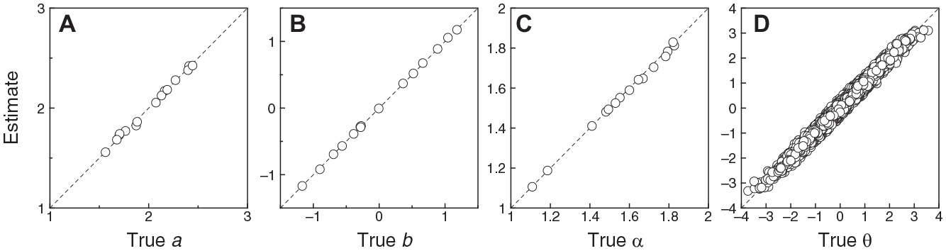
Scatter Plots of Estimated CRM Parameters Against True CRM Parameters for Continuous Data in the Simulation Involving 15 Items and 10,000 Respondents. Each Symbol in Panels (A)–(C) Stands for an Individual Item. Each Symbol in Panel (D) Stands for an Individual Respondent. A Diagonal Identity Line is Plotted for Reference in Each Panel

Deterministic NO-GRM Data

Deterministic conversion of continuous data into Likert data only results in a lower resolution of responses without altering the outcome of the random process by which each continuous response had been generated. In other words, this transformation of continuous data mimics what respondents would do if they reported the continuous response analyzed earlier alongside the interval k into which it falls when discretization boundaries are (y₁, y₂, y₃, y₄) = (0.2, 0.4, 0.6, 0.8).

NO-GRM item parameter and trait level estimates obtained from discretized data are shown in Figure 5 against their counterparts. For item parameters, the counterparts are the NO-GRM item parameters $a_{j}^{*}$ and $b_{j, k}^{*}$ predicted by Equations 5 and 6 from the original CRM parameters; for respondent parameters, the counterparts are the true trait levels that were used to generate the original continuous responses. Item discrimination parameters (Figure 5A) appear to be estimated properly except for a scale factor whereas category threshold parameters (Figure 5B) are estimated at their predicted values. A comparison of Figures 4D and 5C reveals that trait levels at both ends of the continuum are estimated with substantially less precision from discretized data (Figure 5C) than they were from continuous data (Figure 4D). This is easily understandable because respondents with very low (alternatively, very high) trait levels will likely attain the lowest (alternatively, highest) possible score on the Likert version of the test and, then, their trait level estimates will be identical irrespective of differences in their true trait levels. In contrast, the granularity of the continuous response format allows these respondents to obtain different VAS scores that render different trait level estimates for them.

Figure 5.

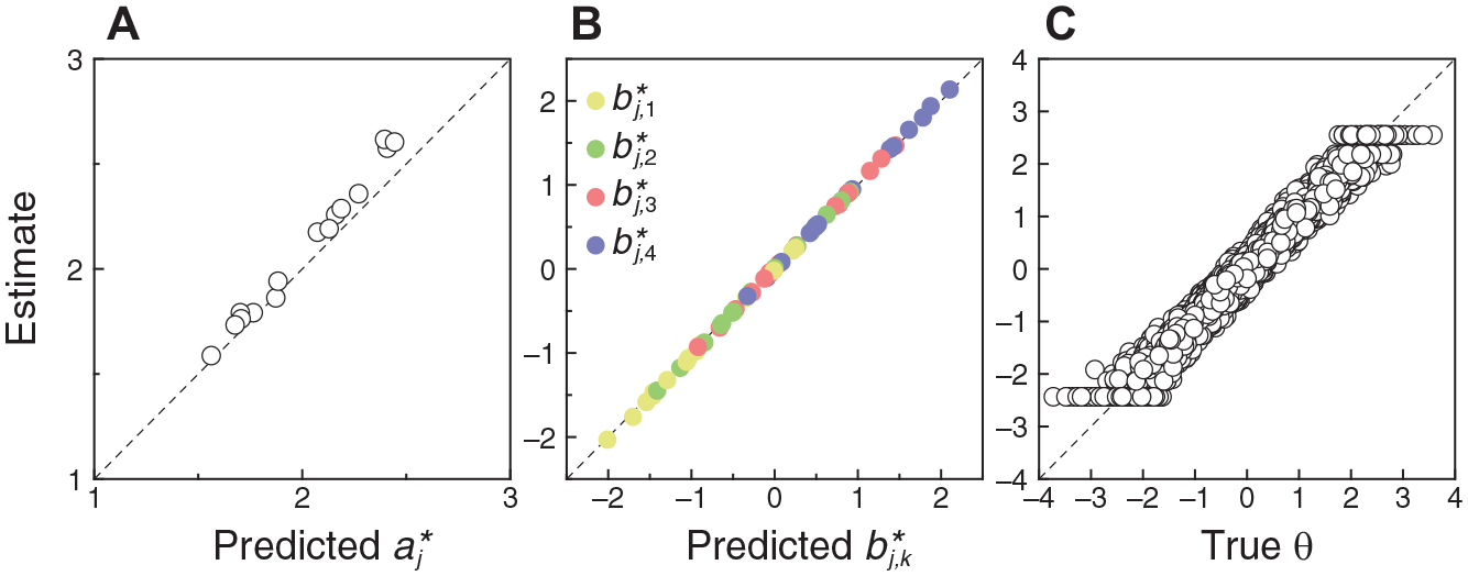
Scatter Plots of Estimated NO-GRM Parameters Against Predicted or True Parameters for Deterministic NO-GRM Data Obtained by Discretization of Continuous Data With (y₁, y₂, y₃, y₄) = (0.2, 0.4, 0.6, 0.8) in the Simulation Involving 15 Items and 10,000 Respondents. Predicted Item Parameters Along the Horizontal Axis in Panels (A) and (B) are Transformations (via Equations 5 and 6) of the CRM Item Parameters with Which the Original Continuous Data Had Been Generated. True Trait Levels Along the Horizontal Axis in Panel (C) are Also Those Used to Generate the Original Continuous data. A Diagonal Identity Line is Plotted for Reference in Each Panel

Yet, it is not immediately obvious why true trait levels in the central range are no more accurately estimated from discretized data (Figure 5C) than they were from continuous data (Figure 4D). As shown in Figure 3, the IIFs of Likert items are higher in the central range than the IIFs of their continuous counterparts. This should hold analogously for the 15 items on this test and it should show in the test information function (TIF), which is the sum of the IIFs. Then, within the central range of trait levels, the standard error of estimation (SE), defined as the inverse of the square root of the TIF, should also be lower in the discrete case and, accordingly, trait estimates should be more accurate. Figure 6 shows the TIF and the SE for the continuous and discretized versions of this 15-item test. The TIF and SE for the continuous version (green horizontal lines) is computed from estimated CRM item parameters and they are indistinguishable from those computed from true parameters, given the estimation accuracy displayed in Figure 4A. The TIF and SE for the discretized version differ slightly when computed from estimated NO-GRM item parameters (red curves) or from true (i.e., predicted from true CRM item parameters via Equations 5 and 6) item parameters (blue curves), owing to the slight mismatch displayed in Figure 5A. Then, despite the clear superiority of the Likert version of the test as regards the TIF in the central range of trait levels (Figure 6A), the actual advantage in terms of expected estimation accuracy in the central range is virtually negligible (Figure 6B).

Figure 6.

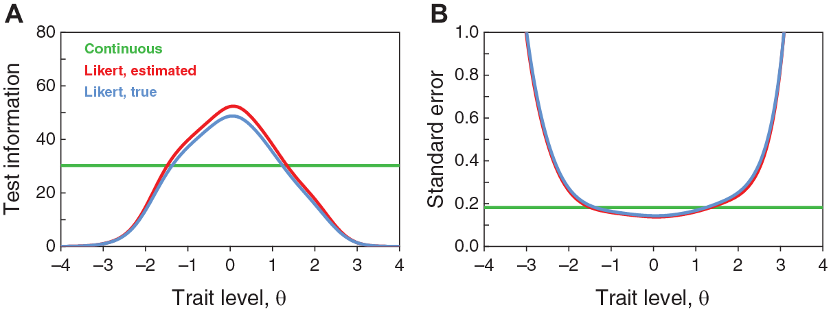
Test Information Functions (A) and Standard Error of Estimation (B) for the Continuous Version of the Test (Green Horizontal Lines) and for the Discretized Version of the Test Using Either Estimated NO-GRM Item Parameters (Red Curves) or True Item Parameters Predicted From True CRM Item Parameters Via Equations 5 and 6 (Blue Curves)

Disengaged NO-GRM Data

Disengaging Likert responses from continuous responses requires replacing the discretized data analyzed in the preceding section with actual Likert data generated by the NO-GRM response process for the same respondents on items whose true parameter values are derived by Equations 5 and 6 from those of their CRM counterparts. To illustrate the differences in approach and to appreciate their potential implications, Figure 7 shows the correspondence between continuous responses and Likert responses obtained in either form. By discretization (Figure 7A), Likert responses are deterministically placed in the category pertaining to the interval on which the original continuous response had fallen. By independent simulation of Likert responses to an item whose NO-GRM parameters are derived via Equations 5 and 6 from the CRM item parameters that produced the continuous data (Figure 7B), continuous responses that had fallen into any given interval may nevertheless be associated with Likert responses in any other category, contingent on the parameters of the NO-GRM item.

Figure 7.

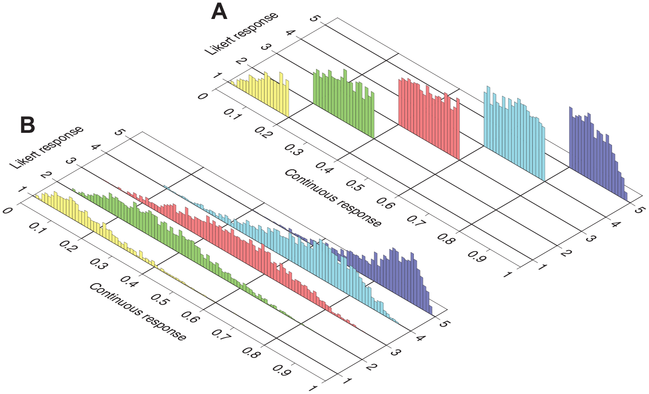
Correspondence Between Continuous Data and Likert Data Obtained in Two Ways. The Height of Each Individual Bar is Proportional to the Number of Respondents (Out of 10,000 in this Simulation) in Each Bin (0.01 Units in Width) Along the Continuous Dimension in Each Likert Category. (A) Likert Data Obtained by Discretizing Continuous Data with Boundaries (y₁, y₂, y₃, y₄) = (0.2, 0.4, 0.6, 0.8), Whose Locations are Immediately Obvious in the Location of the Data. (B) Likert Data Generated by Simulating Discrete Responses to an Item Whose NO-GRM Parameters are Determined From CRM Parameters via Equations 5 and 6 with Boundaries (y₁, y₂, y₃, y₄) = (0.2, 0.4, 0.6, 0.8), Whose Locations are Not Immediately Apparent in the Location of the Data. Continuous Responses are the Same in Both Panels and Pertain to Item 4 in the Simulation. True CRM Item Parameters are a₄ = 3.316, b₄ = −0.288, and α₄ = 1.186; Matching NO-GRM Item Parameters for the Generation of Discrete Data in Panel (B) are $a_{4}^{*}$ = 3.316 and $(b_{4, 1}^{*}, b_{4, 2}^{*}, b_{4, 3}^{*}, b_{4, 4}^{*}) = (- 1.457, - 0.630, 0.054, 0.881)$ . Note that Category Threshold Parameters are Not Equispaced Despite the Equispacing of Discretization Boundaries

In the isolated analysis of disengaged NO-GRM data thus generated, the differences illustrated in Figure 7 in relation to continuous data should be inconsequential. After all, Likert responses are simulated under the NO-GRM for items with known parameters (irrespective of the origin of these parameters) and, then, a comparison of estimated and true item parameters and respondents’ trait levels should indicate typical estimation accuracy for NO-GRM data. Figure 8 shows that this is the case and, in fact, data in each panel of Figure 8 are identical within sampling error to those in the corresponding panel of Figure 5. This is unsurprising on consideration that (a) data in Figure 5 conform to the model in Equation 4 (for discretization of continuous responses) whereas data in Figure 8 conform to the model in Equation 2 (for direct generation of Likert responses) but (b) both models are formally identical and the simulation produced data from matched sets of true parameters. Then, the (minor) differences between results in Figures 5 and 8 only reflect sampling variability. In addition, the slight overestimation of item discrimination parameters that was observed in Figure 5A is clearly not a consequence of discretization of continuous responses, given that it is identically observed in Figure 8A where no discretization was involved. Misestimation of discrimination parameters is ubiquitous in simulations involving graded responses to Likert items (see, for example, García-Pérez, 2017; García-Pérez et al., 2010; Kieftenbeld & Natesan, 2012).

Figure 8.

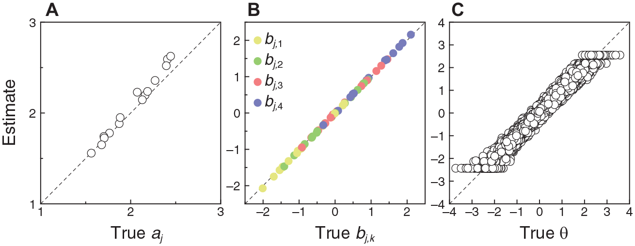
Scatter Plots of Estimated NO-GRM Parameters Against True Parameters for NO-GRM Data Obtained by Independent Simulation of Likert Responses Under the Model of Equation 2, With True Item Parameters Determined via Equations 5 and 6 by the CRM Item Parameters Used to Simulate Continuous Responses, Which Are Not Otherwise Involved Here. Graphical Conventions as in Figure 5

The importance of this simulation strategy is that it allows investigating the possibility of identifying the boundaries y_j,k that are responsible for the characteristics of continuous and Likert data obtained independently, that is, when data are collected from the same sample of respondents and the same set of items separately with VAS and Likert formats. This type of design has been used in a number of studies (e.g., Bolognese et al., 2003; Celenza & Rogers, 2011; Davey et al., 2007; Dourado et al., 2021; Downie et al., 1978; Flynn et al., 2004; Hilbert et al., 2016; Kan, 2009; Kuhlmann et al., 2017; van Laerhoven et al., 2004), although VAS and Likert responses were collected from different samples of respondents in some of them. If a scatter plot of real Likert responses against real continuous responses from the same sample of respondents had the characteristics of Figure 7A, the commonality of response processes as well as the location of the boundaries y_j,k would be immediately obvious. Yet, the few cases in which such plots have been produced reveal instead features similar to those in Figure 7B (see, for example, figure 2 in Celenza & Rogers, 2011; figure 6 in Dourado et al., 2021; figure 3 in Downie et al., 1978; figure 3 in Hilbert et al., 2016), raising the question as to whether the response processes are actually compatible. In a sense, Figure 7B proves that scatter plots with these characteristics are indeed compatible with common item characteristics, which were actually used in the generation of those data. Yet, there is no clear sign in Figure 7B as to what are the boundaries y_j,k sustaining the compatibility, although they can easily be estimated as discussed earlier.

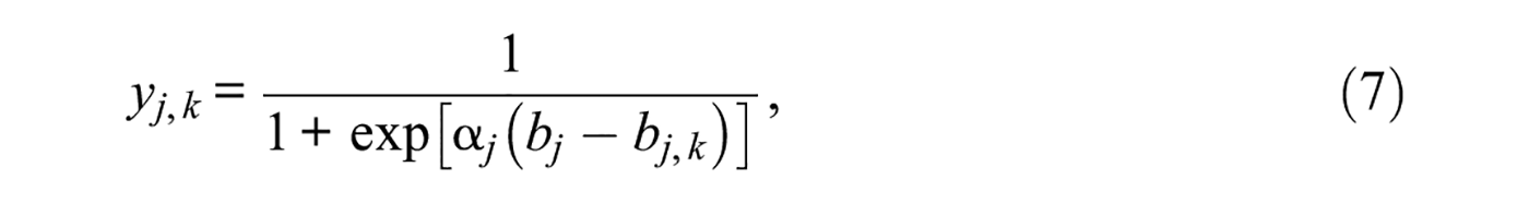
The conditions of this simulation ensure the validity of Equation 6 for true parameter values used in this simulation, but one would also expect this equation to be valid for parameter values estimated from data. The same holds regarding the validity of rearrangement of Equation 6 into Equation 7. Not surprisingly, Figure 9A shows that these relations hold for simulated data: Estimates of discretization boundaries obtained via Equation 7 are in good agreement with the true boundaries (y₁, y₂, y₃, y₄) = (0.2, 0.4, 0.6, 0.8) used to generate the data, which were identical for all items in this simulation. Boundary locations varied randomly across items in other simulation runs and these relations held identically. To illustrate, Figure 9B shows results from an analogous simulation involving 5,000 respondents and also 15 items but now with discretization boundaries that varied across items. To give a flavor of how estimation deteriorates with even fewer data, Figure 9C shows results from a simulation in which 300 respondents took 8 items with discretization boundaries that also varied across items. Despite the substantially smaller number of items and respondents in the latter case, estimated CRM and NO-GRM item parameters still allow acceptable recovery of discretization boundaries for each item via Equation 7.

Figure 9.

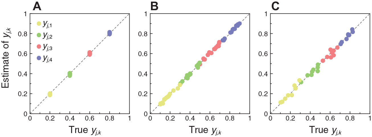
Scatter Plots of Estimated Discretization Boundaries (via Equation 7) Against True Discretization Boundaries y_j,k. The analyses involve simulated data with Likert responses disengaged from continuous responses. (A) Simulation for 10,000 Respondents and 15 Items Sharing Discretization boundaries (y_j,1, y_j,2, y_j,3, y_j,4) = (0.2, 0.4, 0.6, 0.8). (B) Simulation for 5,000 Respondents and 15 Items With Randomly Varying Discretization Boundaries. (C) Simulation for 300 Respondents and 8 Items With Randomly Varying Discretization Boundaries

In sum, Equation 7 is useful to estimate discretization boundaries for each individual item when continuous and Likert responses are both collected for the same set of items in a within-subjects design.

Other Simulation Runs

The simulation whose results have been presented in detail was accompanied by other runs involving the exact same steps for the generation of continuous responses and deterministic versus disengaged generation of Likert responses. These alternative runs differed only as regards the number of respondents (5,000, 1,000, 600, and 300), the number of items (12 and 8), and the locations of discretization boundaries, which could be identical for all items or vary randomly across them. In the latter case, the random location of discretization boundary y_j,k (with 1 ≤k≤K− 1) on the K-category item j was drawn from a uniform distribution on the interval $[\frac{2 k - 1}{2 K}, \frac{2 k + 1}{2 K}]$ .

The results were analogous in all cases except for the accuracy of parameter estimates, which naturally deteriorated as the size of the data sets (i.e., number of respondents and number of items) decreased. For the record, Section 1 of the Supplementary Material provides full graphical results (analogous to those in Figures 4 –8 here) for the most extreme case involving 300 respondents, eight items, and discretization boundaries that vary randomly across items. Note that the recovery of discretization boundaries in this case is already illustrated here in Figure 9C.

Analysis of Empirical Data From Kuhlmann et al. (2017)

Description and Analysis of the Data

Kuhlmann et al. (2017) investigated measurement equivalence of VAS and Likert formats in a within-subjects design involving 879 respondents who took three personality scales under both formats: A Conscientiousness (C) scale with 12 items, an Excitement Seeking (ES) scale with eight items, and a Narcissism (N) scale with six items. Respondents included student attendants to a seminar who were additionally instructed to recruit a minimum of 20 other respondents from the general population in exchange for course credit. There is no reason to think that this recruitment procedure may provide peculiar data in comparison to what other recruitment procedures could have produced. Data for each personality scale were collected on a 5-point Likert scale and on a 101-unit VAS scale, with the order of administration of VAS and Likert response formats counterbalanced across respondents. An unrelated, filler scale involving a free response format was administered to separate the first and second administrations of the personality scales. Kuhlmann et al.’s main research question was stated as “what we gain from implementing VASs as the response format, in comparison to Likert-type response scales” (p. 2175) and their analyses under classical test theory revealed nearly identical psychometric properties of each scale under both response formats as regards means and standard deviations of score distributions, internal consistencies (Cronbach’s alphas) intercorrelations among personality scales, and correlations with age and gender. In other words, no meaningful advantage was associated with the presumably richer VAS response format, at least in terms of the psychometric characteristics of the resultant instrument.

Kuhlmann et al.’s (2017) data are publicly available at https://osf.io/gvqjs and we subjected them to CRM and NO-GRM analyses with our alternative purpose of estimating IRT item parameters and discretization boundaries for each item in each scale. Pre-processing of the data first consisted of removing respondents who had not answered all of the items in both formats on the scale under analysis. This removal left 590, 594, and 599 respondents for the analysis of the C, ES, and N data, respectively. These three separate samples share 570 respondents who answered all items on all scales in both formats. VAS and Likert responses were inverted for items worded in reverse (Items 3, 6, 9, and 11 on the C scale and Items 2 and 4 on the ES scale), and VAS responses were finally rescaled from the original range [1, 101] to the range [0, 1].

CRM and NO-GRM item parameters and respondents’ trait levels were independently estimated for each scale from the corresponding VAS and Likert data, using the software described above for estimation from simulated data. Item parameter estimates for each scale under each IRT model are tabulated in Section 2 of the Supplementary Material. In addition, sum scores were obtained for each respondent in each version of each scale by adding up the Likert scores on each item (each rescaled from the original range [1, 5] to the range [0, 4]) and by adding up the VAS scores that had already been placed in the range [0, 1] for each item.

Results

Comparison of VAS and Likert Data and Their IRT Descriptions

This section starts describing some of the surface-level features of the raw data for which Kuhlmann et al. (2017) had already presented results. These features are displayed here in graphical form to highlight aspects that are relevant to the forthcoming IRT analyses and the check of consistency of the processes underlying VAS and Likert responding.

Figure 10 shows histograms of VAS responses from respondents who marked each Likert category on each item on the ES scale. Analogous plots for all scales are provided in Section 3 of the Supplementary Material. Note that these plots are similar to that in Figure 7B, that is, Likert responses occurred in categories that are not consistent with the interval on which the (independent) VAS response had fallen. Note also that Items 2 and 4 (which were reverse-worded) seem peculiar in that a few respondents gave opposite responses under VAS and Likert formats, that is, responses near one end of the VAS scale and responses near the other end of the Likert scale. This feature was also present in data from the four reverse-worded items on the C scale (Items 3, 6, 9, and 11; see Section 3 of the Supplementary Material). It is not clear whether this is saying something about the (in)convenience of using reverse-worded items alongside other items that are not reverse-worded, but this outcome certainly adds fuel to the controversy over the use of reverse wording (see, for example, García-Fernández et al., 2022; Józsa & Morgan, 2017; Kam, 2023; Suárez-Álvarez et al., 2018; Swain et al., 2008; Vigil-Colet et al., 2020).

Figure 10.

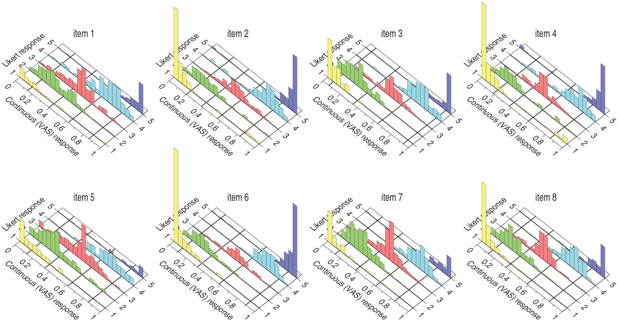
Correspondence Between VAS and Likert Responses for Each Item on the ES Scale. Graphical conventions as in Figure 7. Bin width along the VAS dimension is 0.05 units. Estimated Discretization Boundaries for Each Item Are Indicated by the Lines on the Bottom Plane That Run Along the Likert Dimension at the Corresponding y_j,k Locations Along the VAS Dimension

For a global look at the relation between VAS and Likert scores, Figure 11 shows scatter plots of Likert sum scores against VAS sum scores. The relation is moderately tight along the diagonal line in all scales, although the high values of Pearson correlation seem to overstate the agreement. There are also no signs of nonlinear regimes in these relations. The correlation given in each panel of Figure 11 is nearly identical to the corresponding correlation reported by Kuhlmann et al. (2017) in their table 2. The minute differences are surely due to the different numbers of respondents included for the computations in each case (i.e., respondents who did not omit any item on the two versions of the corresponding scale here versus presumably all respondents in the case of Kuhlmann et al.).

Figure 11.

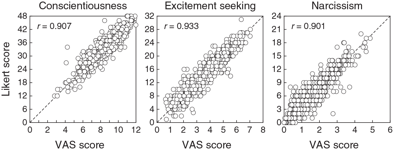
Scatter Plots of Likert Sum Scores Against VAS Sum Scores on Each Scale. Pearson Correlations for Data in Each Panel are Given in the Insets

Turning now to the accuracy of IRT estimates of trait levels and their relation to sum scores, Figure 12 first shows the estimated TIFs and SEs for each of the three scales using CRM and NO-GRM parameter estimates. In contrast to Figure 6 for simulated items with other true parameter values, the VAS format certainly appears to have more potential than the Likert format on all scales throughout the entire range of trait levels, not just at the extremes. Yet, these differences also seem to be largely inconsequential. To illustrate, Figure 13 shows, for each scale, scatter plots of CRM against NO-GRM estimates of trait levels (Figure 13A), VAS sum scores against CRM estimates of trait levels (Figure 13B), and Likert sum scores against NO-GRM estimates of trait levels (Figure 13C). Red curves in Figures 13B and 13C are the test characteristic functions (TCFs) that describe expected test score (given the estimated item parameters) as a function of trait level. Note in Figure 13A that the relation between estimated trait levels under each response format agrees with the corresponding relation between VAS and Likert sum scores (see Figure 11) and the correlations are similarly high. On the other hand, VAS sum scores and CRM estimates of trait levels follow the relation indicated by the TCF for each scale (Figure 13B) and the same holds for Likert sum scores and NO-GRM estimates of trait levels (Figure 13C). Note that the vertical spread around the TCF is smaller in the latter case. The range spanned by the vertical axis in each panel is four times broader in Figure 13C than it is in Figure 13B, but the common size of the vertical axes in these plots reveals that the normalized dispersion of Likert sum scores is smaller than that of VAS sum scores.

Figure 12.

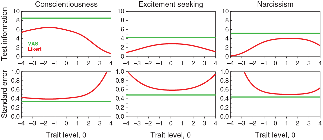
Test Information Functions (Top Row) and Standard Error of Estimation (Bottom Row) for Each Scale (Columns) Under the VAS Format of Administration (Green Lines) and the Likert Format (Red Curves)

Figure 13.

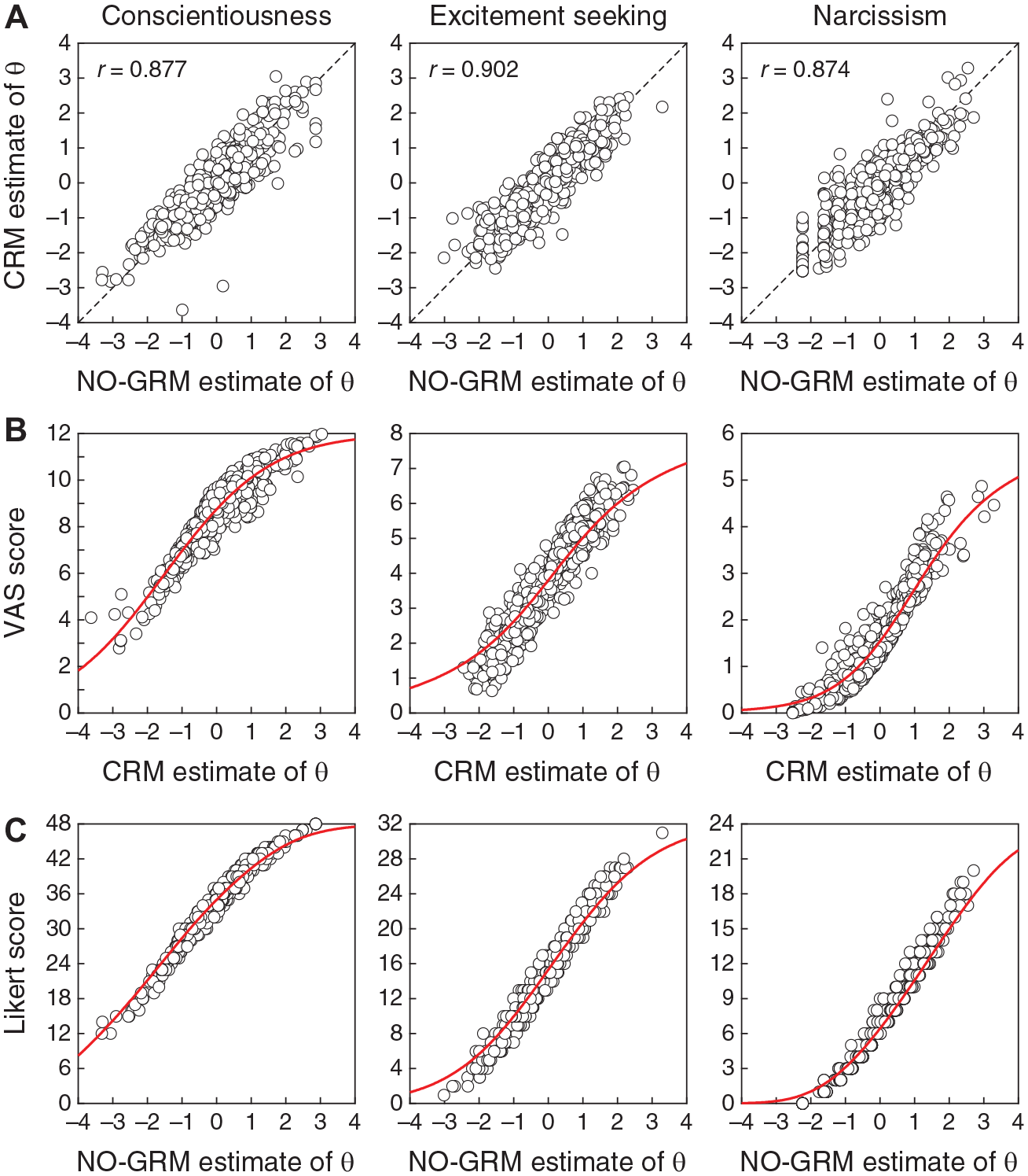
Scatter Plots of Scores and Estimates of Trait Levels for Each Scale (Columns). (A) CRM Estimates of Trait Levels Against NO-GRM Estimates of Trait Levels. Pearson Correlation is Given in the Insets and a Diagonal Line is Plotted for Reference. (B) VAS Scores Against CRM Estimates of Trait Levels. The Red Curve in Each Panel is the Corresponding Test Characteristic Function. (C) Likert Scores Against NO-GRM Estimates of Trait Levels. The Red Curve in Each Panel is the Corresponding Test Characteristic Function

Compatibility of CRM and NO-GRM Accounts of the Data

The preceding results indicate that separate analyses of VAS data under the CRM and Likert data under the NO-GRM result in similar estimates of respondents’ trait levels (see Figure 13A), which surely reflect comparable sum scores under each format of administration (see Figure 11). These results are to be expected if VAS and Likert response processes are actually related as our theoretical analysis surmised, namely, that a VAS response to an item is the result of a draw from the distribution in Equation 3 while a Likert response to the same item is the result of an independent draw from the same distribution that is subsequently discretized according to a partition with the boundaries that hold for the item. Use of Equation 7 to estimate the discretization boundaries for each item from the corresponding CRM and NO-GRM item parameters renders the results shown in Figure 14 for each item on each scale.

Figure 14.

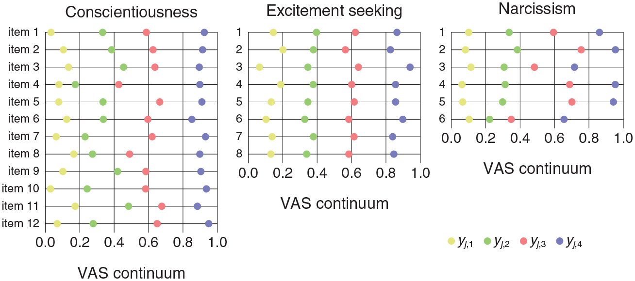
Discretization Boundaries (Colored Circles) for Each Item on Each Scale (Columns). Item Numbers are Indicated on the Left of Each Panel. For Reference, Vertical Lines at Locations 0.2, 0.4, 0.6, and 0.8 Along the VAS Continuum Indicate Where the Boundaries Would Fall for a Partition Into Intervals of the Same Size

Discretization boundaries vary greatly across items and the boundaries within each item are generally away from the locations (vertical lines in each panel) that would provide a partition of the VAS continuum into intervals of the same size. The only case in which boundary locations for all items appear to be placed where an equispaced partition of the VAS continuum would suggest is for boundary y_j,₃ on the ES scale (light red data points in the center panel of Figure 14), but this outcome seems anecdotal given the overall distribution of boundary locations. Discretization boundaries for each of the items on the ES scale had been displayed already in the panels of Figure 10 and they are similarly displayed in analogous panels for the remaining scales in Section 3 of the Supplementary Material.

To further assess the agreement between VAS and Likert response processes, Figure 15 plots the CRFs for each item on the ES scale as directly estimated by the NO-GRM account of Likert data (i.e., Equation 2; black curves) and as predicted from the CRM account of VAS data (i.e., via Equations 4–7; red curves). Analogous plots for all scales are provided in Section 4 of the Supplementary Material. The agreement is not as good as one might have expected, but this is mostly caused by higher estimates of the NO-GRM item discrimination parameters a_j in comparison to their CRM counterparts. Simulations reported above showed that this overestimation occurs also for data generated to comply strictly with common NO-GRM and CRM response processes (see Figures 5A and 8A), despite the fact that Equation 5 dictates item parameters a_j to be identically valued under CRM and NO-GRM characterizations of a given item. In fact, replacing the NO-GRM estimate of a_j for each item with the corresponding CRM estimate resulted in CRFs that superimpose exactly (results not shown), indicating that the remaining item parameters (b_j and α_j from the CRM and b_j,k from the NO-GRM) adhere to the theoretical relation in Equation 6, and keep in mind that these are the only parameters that participate in the estimation of discretization boundaries via Equation 7.

Figure 15.

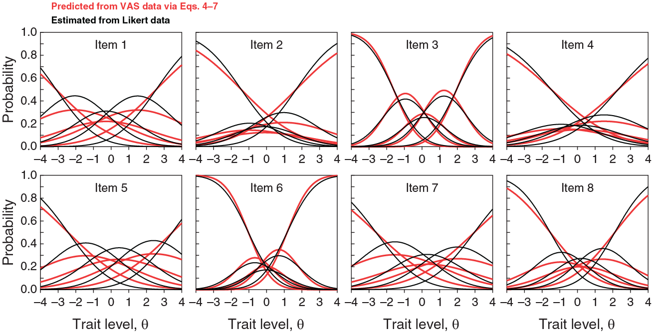
Category Response Functions for the Items on the ES Scale

Discussion

This work set out to investigate the correspondence between continuous (VAS) and discrete (Likert) data provided by the same respondents upon answering the same set of items under both formats. The guiding principle of the study was that every item presumably has unique functional characteristics that are independent of the format of its administration and that these characteristics simply manifest differently under different formats, particularly in the IRT characterization of the items obtained from either data set. The ultimate goal of the study was to use such IRT characterizations to investigate whether the discrete steps inherent to the Likert response format represent equal magnitudes along the underlying dimension, both within and across items.

Summary of Results

A formal analysis first showed that if an item administered with a VAS format conforms to the CRM, then the item has an equivalent expression under the NO-GRM when administered with a K-point Likert format. The functional expressions that relate item parameters under both IRT models were presented and they implicitly incorporate the form in which the VAS continuum is partitioned to generate a Likert response.

Simulations then confirmed that these relations hold in finite samples both when the Likert response is obtained as a mere discretization of the original VAS response and, more realistically, when the Likert response is generated anew and independently from the original VAS response. At the same time, there was no clear sign that estimates of trait levels differ in accuracy according to the format in which the items are administered, with the exception that extreme trait levels were generally estimated more accurately with the VAS format due to the lack of floor and ceiling effects.

An analysis of empirical data from nearly 600 respondents who took three personality scales administered with both response formats revealed characteristics that matched those observed in simulated data, both in terms of the observable aspects of the raw data and in terms of the IRT accounts obtained via CRM and NO-GRM parameter estimates. CRM and NO-GRM item parameters permitted estimating discretization boundaries that map the continuous dimension onto discrete Likert responses. These discretization boundaries differed greatly across items within and across the three personality scales and they generally partitioned the continuum into intervals of different widths. This outcome lends little support to the notion that consecutive steps on a discrete Likert scale represent constant increments in magnitude along the underlying dimension.

Comparison With Earlier Attempts to Investigate the Equal-Interval Assumption

The Introduction mentioned earlier approaches to investigate the equal-interval assumption. These are discussed here in more detail and in relation to the approach taken in this article.

Knutsson et al. (2010) investigated whether the verbal labels (for frequency, intensity, or agreement) that often accompany successive response options on a Likert item are perceived as representing equal increases in magnitude along the underlying continuum. For this purpose, they had respondents indicate such perceived magnitudes on a VAS line. Thus, if each verbally labeled step were perceived to represent the same increase in magnitude, a plot of average VAS setting against (ordered) verbal label would display a linear trend, but their results displayed nonlinear trends instead (see their figure 1).

These results rule out the equal-interval assumption but it should be noted that they provide a global outlook that only applies to the category labels themselves. It is unlikely that the partition that these results reveal will be universal and independent of the specific content of the item with which such labels are used. In contrast, the approach taken in this article allows assessing the form that the partition takes for each individual item on a test, which turned out to differ across items (see Figure 14). Then, even if the category labels for Likert response options did not universally and per se represent steps of equal size on the underlying judgments, item content seems to modulate the relation in ways that need to be assessed on an item-by-item basis.

Toland et al. (2021) took a different route and actually investigated the issue on an item-by-item basis. They administered a four-item test in VAS format and subsequently discretized the responses into K = 10, 5, or 4 categories. Importantly, discretization used intervals of equal and appropriate size in each case, that is, a VAS response Y was converted into the Likert response X = ceil(KY), where ceil(x) is the ceiling function returning the least integer greater than or equal to x. Note that this process yields the outcomes illustrated in Figure 7A above for K = 5 and it works analogously for K = 4 or K = 10. Likert responses subsequently rendered Likert scores by simply subtracting one unit from the Likert responses. Toland et al. then used several polytomous IRT models to estimate category threshold parameters and checked whether the estimated parameter values were equispaced. They did not find the expected equispacing and, then, concluded that the equal-interval assumption does not hold.

Unquestionably, Toland et al.’s results show that estimated category threshold parameters are not equispaced, but it is not at all clear that this fact speaks about the equal-interval assumption. The intervals of concern lie along the response continuum and not along the trait dimension on which category threshold parameters are located. Figure 7 and its legend already showed that equispacing along the response continuum does not render equispaced category threshold parameters. This fact can be easily proved for arbitrary K under the model used here. Specifically, equispacing along the response continuum [0, 1] implies that discretization boundaries are placed at $y_{j, k} = k / K$ for 1 ≤k≤K– 1, bounded by y_j,₀ = 0 and y_j,K = 1 (see Figure 7A for the case in which K = 5). Then, from Equation 6,

\begin{matrix} b_{j, k}^{*} = b_{j} + \frac{\ln (k / K) - \ln (1 - k / K)}{α_{j}} \\ = b_{j} + \frac{\ln (k) - \ln (K - k)}{α_{j}} \end{matrix},

(11)

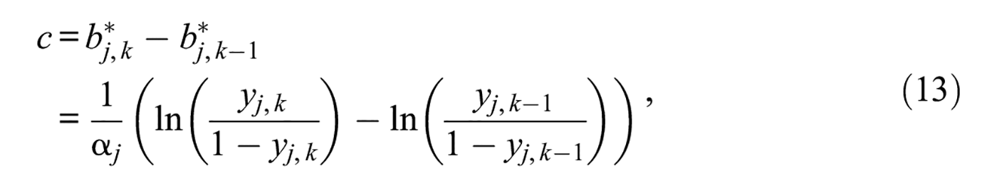
and, thus, the distance between any two consecutive category threshold parameters is

\begin{matrix} b_{j, k}^{*} - b_{j, k - 1}^{*} = \frac{\ln (k) - \ln (K - k)}{α_{j}} - \frac{\ln (k - 1) - \ln (K - k + 1)}{α_{j}} \\ = \frac{1}{α_{j}} \ln (\frac{k (K - k + 1)}{(K - k) (k - 1)}) \end{matrix},

(12)

for 2 ≤k≤K– 1. This distance is not constant across pairs of successive category thresholds despite the fact that the equal-interval assumption holds where it matters, namely, in the discretization of the response continuum. Put another way, equispacing along the response continuum implies that category thresholds are not equispaced under an applicable IRT model. On the other hand, equispacing of category threshold parameters is defined as $b_{j, k}^{*} - b_{j, k - 1}^{*} = c$ for all 2 ≤k≤K– 1. By Equation 6, this implies

\begin{matrix} c = b_{j, k}^{*} - b_{j, k - 1}^{*} \\ = \frac{1}{α_{j}} (\ln (\frac{y_{j, k}}{1 - y_{j, k}}) - \ln (\frac{y_{j, k - 1}}{1 - y_{j, k - 1}})) \end{matrix},

(13)

which holds only when

y_{j, k} = \frac{y_{j, k - 1} \exp [c α_{j}]}{1 - y_{j, k - 1} (1 - \exp [c α_{j}])} .

(14)

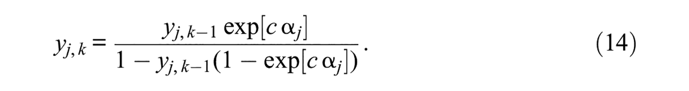
for all 2 ≤k≤K– 1 and, thus, when the response continuum is not partitioned into equal intervals but instead in the form indicated by Equation 14 for any arbitrary location of y_j,₁ and with c < (1 −y_j,₁)/(K− 2).

In sum, checking for equispaced category threshold parameters in IRT models assesses an equispaced partition of the latent trait dimension, but it does not address the question of whether Likert response categories partition the response continuum into intervals of the same size. This applies also to the analogous strategy followed by Sideridis et al. (2023) in their quest for the validity of the equal-interval assumption.

Implications for Scoring of Likert Items

Likert items are scored in the integers from 0 to K– 1 according to the selected response category, with allowance for (spatially) reverse scoring on items that were worded in reverse. This scoring function is justifiable if successive steps along the Likert scale represent constant increments in magnitude both within and across items. Identification of the discretization boundaries y_j,k on each item opens the door to defining a scoring function tailored to each individual item on the test, with potential implications on the dependability and interpretability of the resultant sum scores. For an example, consider the first item on the C scale, for which discretization boundaries were plotted at the top of the left panel in Figure 14 with values (y_1,1, y_1,2, y_1,3, y_1,4) = (0.033, 0.333, 0.587, 0.925). Conventional Likert scores x_j,k, defined as x_j,k = k− 1 for 1 ≤k≤K do not seem to do justice to the partition of the response continuum that the boundaries y_j,k indicate for this item. At first glance, it may seem more reasonable to score a response in category k on item j as the midpoint of the discretization interval for this category on this item (see Müller, 1987), that is,

x_{j, k} = \frac{y_{j, k} + y_{j, k - 1}}{2},

(15)

recalling that y_j,₀ = 0 and y_j,K = 1. The scores thus become (x_1,1, x_1,2, x_1,3, x_1,4, x_1,5) = (0.017, 0.183, 0.460, 0.756, 0.963) for this item. Scores for other items are derived analogously and the scoring function varies across items. Note that use of these scoring functions narrows the range of weighted item scores from the usual [0, K− 1] down to [y_j,₁/2, (1 +y_j,K−₁)/2], which is contained within [0, 1] on all items. A weighted Likert score is equivalent to replacing what the actual VAS setting would have been with the midpoint of the discretization interval on which the VAS setting would have fallen, reducing some of the random variability that would have affected original VAS scores (if they had been collected) and simultaneously reducing the quantization errors embedded in conventional Likert scores obtained by assuming discretization intervals of identical widths. A further advantage of weighted Likert scores is that they eliminate concerns about the absence of interval-scale properties of Likert data, which arise only when steps of different sizes along the continuous response dimension are inadequately scored in constant (unit) steps.

Figure 16 shows weighted Likert sum scores against NO-GRM estimates of trait levels for each of the personality scales, with TCFs (red curves) recomputed accordingly. Compared with the analogous plot involving conventional Likert sum scores (Figure 13C), the relation is slightly tighter here, particularly for the N scale. At the same time, the relation is much tighter than it was in Figure 13B for actual VAS scores.

Figure 16.

Scatter Plots of Weighted Likert Sum Scores Against NO-GRM Estimates of Trait Levels

Although the use of weighted Likert scores as defined above seems more appropriate than the use of conventional Likert scores, the difficulties associated with obtaining the former must be acknowledged. The scoring function in Equation 15 can only be obtained by dual administration of the test in VAS and Likert formats to estimate the needed discretization boundaries y_j,k, a requirement that stands as a serious deterrent except, perhaps, in the development of standardized instruments.

Choice of Response Format

One may ask at this point whether there is any strong evidence supporting a preference for Likert or VAS response formats in practical applications. Ease of administration is no longer a criterion with the current availability of digital technology. The VAS response format has indeed started to be used on the intuition that it provides higher precision (see, for example, Dragan et al., 2022; Liu et al., 2019; Weigl et al., 2021; Wissing & Reinhard, 2018), although no solid evidence to this effect has ever been reported. In contrast, recent and direct evidence reported by Kuhlmann et al. (2017) indicates that scales administered in a within-subjects study with Likert and VAS format do not differ in their score distributions or classical psychometric properties, which shows that the surmised higher precision provided by a continuous response format is only an unfounded myth. Additional analyses reported here of the same data under applicable IRT models show that the continuous VAS format also does not provided any advantage over the discrete Likert format when data are scrutinized from within this alternative framework.

At the same time, there is also no sign that the VAS format brings up issues that should cause concerns to practitioners. These conclusions align with those of other studies in the literature (e.g., Simms et al., 2019). In these circumstances, the choice of format stands only as a matter of convenience or personal preferences with no consequences on the quality of measurement.

The only issue that seems to remain yet unexplored in this context is whether any extra measurement precision can arise from the continuous response format when the VAS line includes intermediate tick marks along its length. In Kuhlmann et al.’s (2017) study, the VAS line was unmarked (see their figure 1), but a recent study has shown that the use of intermediated tick marks help respondents make more accurate settings in comparison with those produced on an unmarked line (García-Pérez & Alcalá-Quintana, 2023). Yet, whether settings that are more accurate results in more accurate measurement is unclear.

Supplemental Material

sj-pdf-1-epm-10.1177_00131644231164316 – Supplemental material for Are the Steps on Likert Scales Equidistant? Responses on Visual Analog Scales Allow Estimating Their Distances

Supplemental material, sj-pdf-1-epm-10.1177_00131644231164316 for Are the Steps on Likert Scales Equidistant? Responses on Visual Analog Scales Allow Estimating Their Distances by Miguel A. García-Pérez in Educational and Psychological Measurement

Footnotes

Declaration of Conflicting Interests

The author declared no potential conflicts of interest with respect to the research, authorship, and/or publication of this article.

Funding

The author disclosed receipt of the following financial support for the research, authorship, and/or publication of this article: This work was supported by grant PID2019-110083GB-I00 from Ministerio de Ciencia e Innovación.

ORCID iD

Miguel A. García-Pérez

Supplemental Material

Supplemental material for this article is available online.

References

Alan

Ü.

Kabasakal

K. A.

(2020). Effect of number of response options on the psychometric properties of Likert-type scales used with children. Studies in Educational Evaluation, 66, 100895. https://doi.org/10.1016/j.stueduc.2020.100895

Bolognese

J. A.

Schnitzer

T. J.

Ehrich

E. W.

(2003). Response relationship of VAS and Likert scales in osteoarthritis efficacy measurement. Osteoarthritis and Cartilage, 11, 499–507. https://doi.org/10.1016/S1063-4584(03)00082-7

Celenza

Rogers

I. R.

(2011). Comparison of visual analogue and Likert scales in evaluation of an emergency department bedside teaching programme. Emergency Medicine Australasia, 23, 68–75. https://doi.org/10.1111/j.1742-6723.2010.01352.x

Davey

H. M.

Barratt

A. L.

Butow

P. N.

Deeks

J. J.

(2007). A one-item question with a Likert or Visual Analog Scale adequately measured current anxiety. Journal of Clinical Epidemiology, 60, 356–360.

Donnellan

M. B.

Rakhshani

(2023). How does the number of response options impact the psychometric properties of the Rosenberg Self-Esteem Scale? Assessment. Advance online publication. https://doi.org/10.1177/10731911221119532

Dourado

G. B.

Volpato

G. H.

de Almeida-Pedrin

R. R.

Oltramari

P. V. P.

Fernandes

T. M. F.

Conti

A. C. C. F.

(2021). Likert scale vs visual analog scale for assessing facial pleasantness. American Journal of Orthodontics and Dentofacial Orthopedics, 160, 844–852. https://doi.org/10.1016/j.ajodo.2020.05.024

Downie

W. W.

Leatham

P. A.

Rhind

V. M.

Wright

Branco

J. A.

Anderson

J. A.

(1978). Studies with pain rating scales. Annals of the Rheumatic Diseases, 37, 378–381. https://doi.org/10.1136/ard.37.4.378

Dragan

W. Ł.

Śliwerski

Folkierska-Żukowska

(2022). New data on the validity of the Fazio Laterality Inventory. PLOS ONE, 17(1), Article e0262803. https://doi.org/10.1371/journal.pone.0262803

Ferrando

P. J.

(2002). Theoretical and empirical comparisons between two models for continuous item responses. Multivariate Behavioral Research, 37, 521–542. https://doi.org/10.1207/S15327906MBR3704_05

10.

Flynn

van Schaik

van Wersch

(2004). A comparison of multi-item Likert and visual analogue scales for the assessment of transactionally defined coping function. European Journal of Psychological Assessment, 20, 49–58. https://doi.org/10.1027/1015-5759.20.1.49

11.

Furukawa

Hojo

Sakamoto

Takaoka

(2021). Modeling response granularity with mixture models: A case of severity ratings in child maltreatment. Behaviormetrika, 48, 393–405. https://doi.org/10.1007/s41237-021-00139-7

12.

García-Fernández

Postigo

Á.

Cuesta

González-Nuevo

Menéndez-Aller

Á.

García-Cueto

(2022). To be direct or not: Reversing Likert response format items. Spanish Journal of Psychology, 25, E24. https://doi.org/10.1017/SJP.2022.20

13.

García-Pérez

M. A.

(2017). An analysis of (dis)ordered categories, thresholds, and crossings in difference and divide-by-total IRT models for ordered responses. Spanish Journal of Psychology, 20, E10. https://doi.org/10.1017/sjp.2017.11

14.

García-Pérez

M. A.

Alcalá-Quintana

(2023). Accuracy and precision of responses to visual analog scales: Inter-and intra-individual variability. Behavior Research Methods. Advance online publication. https://doi.org/10.3758/s13428-022-02021-0

15.

García-Pérez

M. A.

Alcalá-Quintana

García-Cueto

(2010). A comparison of anchor-item designs for the concurrent calibration of large banks of Likert-type items. Applied Psychological Measurement, 34, 580–599. https://doi.org/10.1177/0146621609351259

16.

Gideon

Helppie-McFall

Hsu

J. W.

(2017). Heaping at round numbers on financial questions: The role of satisficing. Survey Research Methods, 11, 189–214. https://doi.org/10.18148/srm/2017.v11i2.6782

17.

Hilbert

Küchenhoff

Sarubin

Nakawaga

T. T.

Bühner

(2016). The influence of the response format in a personality questionnaire: An analysis of a dichotomous, a Likert-type, and a visual analogue scale. TPM—Testing, Psychometrics, Methodology in Applied Psychology, 23, 3–24. https://doi.org/10.4473/TPM23.1.1

18.

Józsa

Morgan

G. A.

(2017). Reversed items in Likert scales: Filtering out invalid responders. Journal of Psychological and Educational Research, 25, 7–25.

19.

Kam

C. C. S.

(2023). Why do regular and reversed items load on separate factors? Response difficulty vs. item extremity. Educational and Psychological Measurement. Advance online publication. https://doi.org/10.1177/00131644221143972

20.

Kan

(2009). Effect of scale response format on psychometric properties in teaching self-efficacy. Eurasian Journal of Educational Research, 34, 215–228.

21.

Kieftenbeld

Natesan

(2012). Recovery of graded response model parameters: A comparison of marginal maximum likelihood and Markov Chain Monte Carlo estimation. Applied Psychological Measurement, 36, 399–419. https://doi.org/10.1177/0146621612446170

22.

Kinley

(2022). A jsPsych plugin for visual analogue scales. PsyArXiv. https://doi.org/10.31234/osf.io/avj92

23.

Knutsson

Rydström

Reimer

Nyberg

Hagell

(2010). Interpretation of response categories in patient-reported rating scales: A controlled study among people with Parkinson’s disease. Health and Quality of Life Outcomes, 8, 61. http://www.hqlo.com/content/8/1/61

24.

Krosnick

J. A.

(1991). Response strategies for coping with the cognitive demands of attitude measures in surveys. Applied Cognitive Psychology, 5, 213–236. https://doi.org/10.1002/acp.2350050305

25.

Kuhlmann

Dantlgraber

Reips

U.-D.

(2017). Investigating measurement equivalence of visual analogue scales and Likert-type scales in Internet-based personality questionnaires. Behavior Research Methods, 49, 2173–2181. https://doi.org/10.3758/s13428-016-0850-x

26.

Liu

Peterson

A. C.

Wing

Crump

Younger

Penner

Veljkovic

Foggin

Sutherland

J. M.

(2019). Validation of the Ankle Osteoarthritis Scale instrument for preoperative evaluation of end-stage ankle arthritis patients using item response theory. Foot & Ankle International, 40, 422–429. https://doi.org/10.1177/1071100718818573

27.

Maydeu-Olivares

Kramp

García-Forero

Gallardo-Pujol

Coffman

(2009). The effect of varying the number of response alternatives in rating scales: Experimental evidence from intra-individual effects. Behavior Research Methods, 41, 295–308. https://doi.org/10.3758/BRM.41.2.295

28.

Müller

(1987). A Rasch model for continuous ratings. Psychometrika, 52, 165–181. https://doi.org/10.1007/BF02294232

29.

Müssig

Kubiak

Egloff

(2022). The agony of choice: Acceptance, efficiency, and psychometric properties of questionnaires with different numbers of response options. Assessment, 29, 1700–1713. https://doi.org/10.1177/10731911211029379

30.

Preston

C. C.

Colman

A. M.

(2000). Optimal number of response categories in rating scales: Reliability, validity, discriminating power, and respondent preferences. Acta Psychologica, 104, 1–15. https://doi.org/10.1016/S0001-6918(99)00050-5

31.

Reips

U.-D.

Funke

(2008). Interval-level measurement with visual analogue scales in Internet-based research: VAS generator. Behavior Research Methods, 40, 699–704. https://doi.org/10.3758/BRM.40.3.699

32.

Samejima

(1969). Estimation of latent ability using a response pattern of graded scores (Psychometric Monograph No. 17). Psychometric Society. http://www.psychometrika.org/journal/online/MN17.pdf

33.

Samejima

(1973). Homogeneous case of the continuous response model. Psychometrika, 38, 203–219. https://doi.org/10.1007/BF02291114

34.

Samejima

(2005). Graded response model. In Kempf-Leonard

(Ed.), Encyclopedia of social measurement (Vol. 2, pp. 145–153). Elsevier. https://doi.org/10.1016/B0-12-369398-5/00451-5

35.

Shi

Siceloff

E. R.

Castellanos

R. E.

Bridges

R. M.

Jiang

Flory

Benson

(2021). Revisiting the effect of varying the number of response alternatives in clinical assessment: Evidence from measuring ADHD symptoms. Assessment, 28, 1287–1300. https://doi.org/10.1177/1073191120952885

36.

Shojima

(2005). A noniterative item parameter solution in each EM cycle of the continuous response model. Educational Technology Research, 28, 11–22. https://doi.org/10.15077/etr.KJ00003899231

37.

Sideridis

Tsaousis

Ghamdi

(2023). Equidistant response options on Likert-type instruments: Testing the interval scaling assumption using Mplus. Educational and Psychological Measurement. Advance online publication. https://doi.org/10.1177/00131644221130482

38.

Simms

L. J.

Zelazny

Williams

T. F.

Bernstein

(2019). Does the number of response options matter? Psychometric perspectives using personality questionnaire data. Psychological Assessment, 31, 557–566. https://doi.org/10.1037/pas0000648

39.

Suárez-Álvarez

Pedrosa

Lozano

L. M.

García-Cueto

Cuesta

Muñiz

(2018). Using reversed items in Likert scales: A questionable practice. Psicothema, 30, 149–158. https://doi.org/10.7334/psicothema2018.33

40.

Swain

S. D.

Weathers

Niedrich

R. W.

(2008). Assessing three sources of misresponse to reversed Likert items. Journal of Marketing Research, 45, 116–131. https://doi.org/10.1509/jmkr.45.1.116

41.

Toland

M. D.

Kodet

Reese

R. J.

(2021). Psychometric properties of the outcome rating scale: An item response theory analysis. Measurement and Evaluation in Counseling and Development, 54, 90–105. https://doi.org/10.1080/07481756.2020.1745647

42.

van Laerhoven

van der Zaag-Loonen

H. J.

Derkx

B. H. F.

(2004). A comparison of Likert scale and visual analogue scales as response options in children’s questionnaires. Acta Paediatrica, 93, 830–835. https://doi.org/10.1111/j.1651-2227.2004.tb03026.x

43.

Vickers

A. J.

(1999). Comparison of an ordinal and a continuous outcome measure of muscle soreness. International Journal of Technology Assessment in Health Care, 15, 709–716. https://doi.org/10.1017/S0266462399154102

44.

Vigil-Colet

Navarro-González

Morales-Vives

(2020). To reverse or to not reverse Likert-type items: That is the question. Psicothema, 32, 108–114. https://doi.org/10.7334/psicothema2019.286

45.

Wang

Zeng

(1998). Item parameter estimation for a continuous response model using an EM algorithm. Applied Psychological Measurement, 22, 333–344. https://doi.org/10.1177/014662169802200402

46.

Weigl

Schartmüller

Riener

Steinhauser

(2021). Development of the Questionnaire on the Acceptance of Automated Driving (QAAD): Data-driven models for Level 3 and Level 5 automated driving. Transportation Research Part F: Traffic Psychology and Behaviour, 83, 42–59. https://doi.org/10.1016/j.trf.2021.09.011

47.

Wissing

B. G.

Reinhard

M. A.

(2018). Individual differences in risk perception of artificial intelligence. Swiss Journal of Psychology, 77, 149–157. https://doi.org/10.1024/1421-0185/a000214

48.

Zopluoglu

(2012). EstCRM: An R package for Samejima’s continuous IRT model. Applied Psychological Measurement, 36, 149–150. https://doi.org/10.1177/0146621612436599

49.

Zopluoglu

(2013). A comparison of two estimation algorithms for Samejima’s continuous IRT model. Behavior Research Methods, 45, 54–64. https://doi.org/10.3758/s13428-012-0229-6

Supplementary Material

Please find the following supplemental material available below.

For Open Access articles published under a Creative Commons License, all supplemental material carries the same license as the article it is associated with.

For non-Open Access articles published, all supplemental material carries a non-exclusive license, and permission requests for re-use of supplemental material or any part of supplemental material shall be sent directly to the copyright owner as specified in the copyright notice associated with the article.

0.00 MB

0.64 MB