Sage Journals: Discover world-class research

Abstract

Many jurisdictions across the U.S. have adopted justice reinvestment initiatives (JRIs) as a strategy for reducing the use of incarceration and mitigating large correctional budgets. In spite of this widespread adoption, little empirical research has explored the impacts of justice reinvestment policies. In response, this study employed quasiexperimental, interrupted time-series regression analyses using a decade of monthly court and corrections data to assess if JRI legislation in Oregon was effective. Results show decreased prison usage and recidivism, as well as reveal delayed and significant trend changes for felony jail admissions and community corrections populations as a result of the JRI legislations. A course for future research to further advance understanding of reinvestment and resource reallocation is outlined.

Keywords

justice reinvestment policy sentencing community supervision recidivism

Although the imprisonment rate in the United States has dropped 9% from 2008 to 2018, there are still roughly 1.5 million people incarcerated in state and federal prisons (American Civil Liberties Union Foundation, 2015; Carson, 2020). During the same time, crime rates continued to fall (Federal Bureau of Investigation, 2021). According to a 2015 Vera Institute of Justice survey, the average annual cost per prisoner was $33,274 (Mai & Subramanian, 2017), which cumulatively equated to total prison expenditures of $43 billion per year. Additionally, recent reports by the Bureau of Justice Statistics estimate more than 4.5 million people are on community supervision (Kaeble & Cowhig, 2018). While operation costs are much lower for community versus institutional settings, there is concern that these costs are deferred for only a short period as about two-thirds of those released to supervision are eventually returned to prison (U.S. Department of Justice, 2017). Moreover, a growing body of scholarship suggests that imprisonment produces only a marginal effect on crime rates and recidivism (Rydberg & Clark, 2016) or a criminogenic effect (Petrich et al., 2021). High rates of returns to custody embody a “revolving door” of corrections (Freeman, 2003), which place strain on custodial systems and increases their operational costs. Concerns about costs and efficiency have inspired many jurisdictions to search for strategies that can reduce prison use while also ensuring public safety.

One way that some state governments have sought to reduce their prison population and correctional costs is through the use of Justice Reinvestment Initiatives, or JRIs (see Bureau of Justice Assistance [BJA], 2014). The concept of justice reinvestment refers to a policy that attempts to reduce inefficiencies in the criminal justice system and divert convicted individuals from prison in order to accumulate fiscal savings, which can then be invested into high incarceration communities. In practice, these saved (or averted) funds are re-invested into rehabilitative and reentry programs with the goal to reduce both recidivism and long-term correctional costs (Sabol & Baumann, 2020). With oversight provided by the Bureau of Justice Assistance (BJA), the JRI reform efforts have now been implemented in at least 35 states (Pew Charitable Trusts, 2018). Despite the growing popularity of JRIs, however, there has been little empirical research on the results of these policies (Sabol & Baumann, 2020). This study provides an evaluation of the impact of a statewide JRI effort—Oregon’s House Bill (HB) 3194 (henceforth Justice Reinvestment Act, or JRA). We examine the effects of JRA on prison population, jail usage, community supervision, and recidivism using an interrupted time series regression analysis.

Literature Review

Origins of Justice Reinvestment

First introduced in 2003, justice reinvestment was posited to suggest that reducing incarceration usage and redirecting the savings into “rebuilding [. . .] human resources and physical infrastructure” would yield lower long-term crime rates (Tucker & Cadora, 2003, p. 3). Tucker and Cadora argued that successful reinvestment requires funds to be redistributed across four areas: community development, education, health, and rehabilitation and reentry services. Further, they suggest that investment in these areas can sustain reductions in incarceration and provide substantial benefits to communities. This strategy of justice reinvestment relies on all types of reinvestment to produce lasting change and to minimize the impact of our prison system (Tucker & Cadora, 2003). In contrast, the implementation of justice reinvestment practices has been less structured by specific definition and more by broad strategic plans. As Clear (2011) has discussed, these plans inherently leave many details unaddressed, such as how presumptive prison defendants are diverted, what constitutes savings, and how funds are to be reinvested. These factors have allowed for a wide variation in JRI practice (e.g., reinvesting in either community based substance abuse treatment or reentry housing). Common strategies often involve varying efforts for reinvesting in evidence-based programs to reduce recidivism rather than investing in human resources and infrastructure for non-criminal justice areas.

In one of the earliest known efforts of justice reinvestment, Connecticut reinvested approximately $13 million into reentry programs in 2004, with the goal to reduce probation and parole populations and create automatic parole hearings after 85% time-served (Council of State Governments [CSG], 2017a). The reforms were later hailed as the reason Connecticut had one of the fastest decreasing incarcerated populations in the nation, although this conclusion was based largely on descriptive statistics which fails to account for the importance of nuanced change and cannot be critically compared to other trends (CSG, 2017a). Similar practices were observed in other states (e.g., Texas; Orrick & Vieraitis, 2015) and many government officials began to recognize the appeal of justice reinvestment (Clear, 2011). Ultimately, in 2010 Congress allocated funding to the BJA to create the JRI to “fund, coordinate, assess, and disseminate state and local justice reinvestment efforts” (La Vigne et al., 2014, p. 6). The initiative officially transitioned the reinvestment focus from communities and crime prevention to jurisdiction-based technical assistance (Sabol & Baumann, 2020). To date, JRI has provided technical assistance and funding to local and state stakeholders, who aim to craft solutions for the specific needs of each jurisdictions (Harvell et al., 2016).

In an Urban Institute report on the manifestation of justice reinvestment in policy reform, Harvell et al. (2016) noted that 24 states enacted five general types of reforms: (1) amendments to sentencing laws, (2) the restructure of pretrial practices, (3) modification of prison release practices, (4) strengthening community corrections, and (5) amendments that ensure the sustainability of reforms (pp. vi–vii). Amendments to sentencing laws have taken the form of diverting low-level, often non-violent, prison-presumptive cases toward probation rather than prison, or an outright repeal of mandatory minimum sentences. Pretrial reform has emphasized reducing the use of pretrial detention given the demonstrated negative effects it can have on sentencing (e.g., Campbell et al., 2020; Oleson et al., 2016). Modified release practices have various structure and results. For instance, Montana implemented early release and found it was associated with increased recidivism (Wright & Rosky, 2011). Regardless of outcome, modifying release practices and the diversion of presumptive prison cases has encouraged some jurisdictions to strengthen their community corrections capacity. Largely out of necessity with more cases on community supervision, Harvell et al. (2016) emphasized that most initiatives have pushed officials to use risk and needs assessments to help guide supervision, treatment, violation-responses, and decisions. Of these reform areas, jurisdictions have implemented varying arrays that emphasize one reform or combine multiple types. While such efforts may result in JRI achieving its goals, the variation has made evaluation difficult.

Two of the paramount difficulties in evaluating justice reinvestment stem from calculating generated or averted savings and tracking prison populations. First, the primary enabling mechanism for reinvestment, avoided costs/generated savings, has been largely inaccessible to researchers. Many of the jurisdictions (16 states) rely on legislative mandates to earmark funds specifically for justice reinvestment but they are ambiguous to the future allocation of saved monies (e.g., Delaware or Missouri; Austin & Coventry, 2014; Harvell et al., 2016). An evaluation that tracked averted costs estimated the savings for all JRI states totaled roughly $1 billion in 2016 (Harvell et al., 2016); a figure far below what was pitched by proponents of JRI (see Austin et al., 2013; Sabol & Baumann, 2020). Second, most empirical assessments have focused on assessing the impacts on correctional populations, leaving less known about the effects on recidivism. Of published evaluations, many highlight corrections population counts broadly that have either stabilized or decreased following JRI implementation (CSG, 2017b; Harvell et al., 2016; La Vigne et al., 2014). Further, Sabol and Baumann (2020) explain that the comparison of projections can be quite misleading when trying to determine impact for prison populations because results range widely between states.

To compound these issues, many of these estimated effects are problematic (Sabol & Baumann, 2020). One prominent issue is the omission of adequate pre-JRI data in the projections (Austin & Coventry, 2014; Austin et al., 2013). Omitting adequate pre-intervention data can lead to inaccurate comparisons and conclusions about success and failure of the policy (Zhang et al., 2011). Moreover, such comparisons often overlook possibly stagnant prison population growth prior to JRI implementation. Sabol and Baumann (2020) have argued that claims of JRI success often overlook the observation that, in 18 of the participating JRI states, prison populations were already slightly declining before implementation even began.

Justice Reinvestment in Oregon

Between 2000 and 2010, Oregon’s prison population grew from 9,491 to 13,784 adults in custody, an increase of nearly 45% (BJA, 2014). With concern mounting over the possible need to build a new prison by 2014 (Schmidt, 2017), Oregon joined the JRI technical assistance program sponsored by the BJA in 2012. After an extensive review of criminal justice policy, practices, and costs, HB 3194 was passed by the legislature in July 2013. The governor signed the law into effect on July 23, 2013 by issuing a declaration of emergency (JRA, 2013). The JRA has three primary parts: goals, structural reforms (sentencing and supervision), and the reinvestment grant.

First, the Justice Reinvestment Act sets out four primary goals to guide its creation and execution across the state. These are to (1) decrease prison usage and (2) reduce recidivism while (3) maintaining public safety and (4) holding offenders accountable (Oregon CJC, 2018). Despite these requirements, few programs and processes have been evaluated for their attainment of the legislature’s four desired outcomes or in their effectiveness in achieving their own goals.

Second, the JRA addressed a number of sentencing reforms and correctional restructuring. These include reducing the criminal penalties for marijuana offenses (excluding commercial quantities), driving with a suspended license, robbery in the third degree, and identity theft. In addition to sentencing reforms, the bill expanded short term transitional leave (early release from prison) from 30 to 90 days prior to discharge. The Act also restructured the accumulation of behavior-related time credits while on supervision and constrained it to be no greater than 50% of the supervision period. Finally, this law repealed the prohibition of dispositional downward departure that was established previously (see Oregon’s Measure 57, 2008). These direct changes to the sentencing structure and the accumulation of sentence reductions for both incarcerated persons and persons under community supervision went into effect immediately due to the emergency clause in the bill. The nature of these reforms aligns with the assessments above that states have mostly made changes to sentencing structures (Harvell et al., 2016). These changes, in conjunction with tripling early release from prison, may have the most direct impact on the prison population.

Third, the act also created the justice reinvestment grant and requires the Oregon Criminal Justice Commission (CJC) to distribute grant funds each biennium for implementation and support of evidence-based practices.¹ While the law states that funding should be distributed to counties that implement programming based on the ability of the practice to achieve the legislature’s goals, the legislature ultimately tied the distribution of grant funding to the proportion of the prison population that each county contributes to state total. This means that counties that are the largest contributors to the prison population get the most funds from the justice reinvestment grant. This study will evaluate at the state level if the distribution of grant funds, as a policy, is associated with changes in population variables and recidivism.

According to a CJC report, the state’s prison population had remained relatively flat since the JRA’s passage (Schmidt & Officer, 2015). This trend was projected to remain below the threshold required to build a new prison by the end of 2017 (Schmidt & Officer, 2015). The Oregon Task Force on Public Safety (OTFPS) released an outcome evaluation in 2016 indicating that of all changes made by the JRI legislation, short-term transitional leave was the only change that achieved its projected savings. All other sentencing changes achieved little to no fiscal savings (OTFPS, 2016). Additional reports by the CJC have focused on the avoided costs and expenditures of the justice reinvestment grant program (Schmidt, 2017). Evidence suggests that JRA avoided almost $20 million in state Department of Corrections (DOC) costs between 2013 and 2015. Analyses also suggest that, in total, the estimated net cost avoidance for justice reinvestment between 2013 and 2019 is projected to be $254 million (Schmidt, 2017).

Current Study

Although JRI has been widely implemented in some form across the nation, there is scant research available that examines efforts at the state level. Evaluations to date consist largely of descriptive breakdowns or assessments of individual programmatic effects in municipalities. Moreover, in spite of Oregon’s reporting to date, no rigorous, large scale analyses have been completed on the effects of JRI across the state. This study uses interrupted time series (ITS) regression analysis in a rigorous, quasi-experimental examination of Oregon’s justice reinvestment efforts. Macro(state)-level analysis is a natural entry to the examination of justice reinvestment for several reasons. First, much of the existing literature is comprised of macro analyses that employ a myriad of methods that have been critiqued as discussed earlier (Austin et al., 2013; Sabol & Baumann, 2020). Therefore, one of the aims of this study is to apply a replicable method that forms a clear baseline for comparison—the counterfactual—on the same level as other studies (Austin & Coventry, 2014; Austin et al., 2013). Second, and perhaps more important, is the nature of the JRA itself: The major changes that should produce savings and down-the-line funding opportunities are generated by sentencing changes applied by the legislature at the state level; and should therefore have little micro (county)-level implementation variance. Finally, any analysis of micro-level jurisdictional implementation (by either county or judicial district) would be incomplete without relating how those findings interact to comprise macro results. Therefore, understanding how macro-level goals have changed can inform future research that evaluates the effects of uneven funding distribution and differencing implementation that represents the “black box” of justice reinvestment at a micro-level.

In this investigation, we examine the first two goals of prison use and recidivism. The third goal, maintaining public safety, will require a focused analysis that is beyond the current presentation due to data constraints and agency reporting issues (Federal Bureau of Investigation, 2015).² Included in Appendix Figure 1 is a yearly depiction of crime in Oregon, which largely did not change over the observation period. The fourth goal, holding offenders accountable, would also require a categorically different and nuanced approach to study structure and data sources. As such, the current study is limited to the goals of decreasing prison usage and reducing recidivism. Additionally, we will evaluate the potential latent consequences in jail and community supervision to evaluate the effectiveness of Oregon’s JRA thus far. To our knowledge, no other study has used ITS regression to evaluate the aggregate statewide effectiveness of a JRI reform. Here we examine 10 years of data acquired monthly beginning in 2008, 5 years before the JRA was enacted and for 5 years after its enactment to begin to answer the question: Has the Oregon JRA been effective in reducing prison use and recidivism?

Considering the goals of the Oregon Justice Reinvestment Act, we expect the prison population to significantly decrease over time (H₁). As jurisdictions implement justice reinvestment efforts to divert people away from prison, it is possible that they will divert those newly convicted to jail or community supervision (Underwood et al., 2020). As a result, we expect to see, at least in the short to intermediate term (i.e., 6–18 months), a significant increase in felony jail admissions (H₂). We also expect a concomitant increase in admission to community supervision (H₃). Over time, if reinvestment is successful, we expect to see a reduction in recidivism (H₄). For the purposes of this examination and as specified in the JRA, we focus on the recidivism rate as defined by the state in three ways: rearrest, reconviction, and reincarceration within 3 years of release to the community. Therefore, we expect a significant decrease in all types of recidivism. For the JRA to be effective the prison population and rate of recidivism should decrease while an increase in felony jail admissions and/or community supervision should be short-term artifacts of start-up.

Method

Data

We obtained deidentified data, aggregated monthly, from the Oregon CJC and publicly available data from the Oregon DOC. All population based rates used in this study were constructed by calculating the average monthly change for U.S. Census population estimates in each year from 2000 through 2017 (U.S. Census Bureau, 2018).³ For each dependent measure examined, the monthly count was divided by the state’s monthly estimated population and multiplied by 100,000. Over this period, the population of Oregon increased by 8% between 2010 and 2017. We collected ten years of monthly data, five before the intervention of the JRA (June 2008–June 2013) and five after the intervention (July 2013–July 2018).

The Intervention: Justice Reinvestment

The primary independent variable in ITS analyses is the introduced intervention. In this study, the intervention is set to be the JRA enrollment month, July 2013, because the data are aggregated monthly. A dummy variable is used to describe the impact of the intervention (see Fox, 2016, Ch. 7; McCleary et al., 2017; McDowall et al., 1980). It is unlikely the JRA had an immediate impact given the time lag required for the CJC to evaluate programs, to create the infrastructure to distribute funds, and then to distribute funds to participating jurisdictions. Additionally, the JRA has not been repealed since its enrollment. Therefore, the impact will likely have a gradual and permanent effect on the dependent variables. Estimation of this gradual and permanent structure is achieved in two parts.

First, an independent variable, here named “Level,” is dichotomously coded as 0 if prior to the enrollment of the JRA and 1 on the intervention date and afterward. This variable is used to represent the presence of the JRA in the regression model. Second, a variable, “Trend,” is a counter variable, set to 0 when the intervention is not present and sequentially counting upwards (1, 2, 3, . . .) for each month after the intervention. This variable is used to estimate the rate of change post intervention. Therefore, the combination of the two independent variables allows a gradual (trend) and permanent (level) impact pattern to be tested; modeled by a possibly non-significant immediate impact and a significant trend change. The strength of regression in ITS analyses is that the researcher need not assume the structure of the effect for the event or intervention. For example, the dependent time series might exhibit a minor abrupt change due to the restructuring of the classification of crimes, but the funding and implementation of evidence-based practices may have required a greater amount of time. This suggests a gradual change in the dependent measures (McCleary et al., 2017; McDowall et al., 1980).

Dependent Variables

Dependent variables in ITS analyses are the measures for which the intervention may have an effect. The language of the JRA directly calls for measuring four goals: reducing prison usage, reducing recidivism, maintaining public safety, and holding offenders accountable. To date there has not been a defensible definition of “holding offenders accountable” and is therefore not included in the outcomes tested in this study. Additionally, due to changes in instrumentation during the study period, crime data were unable to be collected (there is a data gap for 2015 for nearly all UCR reporting in Oregon). Therefore, the dependent measures used to evaluate the goals of the JRA are prison rate and recidivism. Count data are reported only for the prison population because the DOC count and rate data differ in structure while all other count and rate variables are structurally similar. Rates are used in this study for two related reasons.⁴ Population based rates allow the results to be compared across disparate jurisdictions with different need-based priorities and policies (Dollar, 2018). Additionally, results expressed on a per 100,000 basis may facilitate comparisons between individual counties or states engaging in JRI programs.

Prison counts and rates

Data containing a monthly count of all people housed in prison are publicly available and published by the Oregon DOC (2019). These data are the total number of individuals in prison each month. To determine the change in the rate of prison use, counts were transformed into a rate using the population of Oregon (U.S. Census Bureau, 2018) and a base of 100,000. Controlling for population growth is imperative as the population has substantially increased over the two decades (U.S. Census Bureau, 2021).

Felony jail admission rate

The felony jail population variable involved aggregate jail admissions for individuals with a felony conviction (i.e., property, driving, drug possession, drug, person, sex, and other). The felony jail admissions rate was calculated by dividing the monthly count of convicted individuals serving their sentences in local control by the state population then multiplying by 100,000.

Community supervision rate

The community supervision population was calculated by adding the total number of individuals on probation and post-prison supervision as identified by Oregon DOC (2019). Individuals are counted on probation if they were convicted of a felony offense, have only a probation sentence (i.e., did not also receive a prison sentence for a charge on the same case), and are placed on community supervision (i.e., may have jail time but did not get revoked to prison).⁵ Post-prison supervision consists of all convicted individuals who are serving a determinately sentenced term of supervision following release from institutional custody.

Recidivism rate

The recidivism data were analyzed by “matured” monthly cohorts that allow for at least 3 years of post-intervention follow-up (July 2013–June 2016). Deidentified individual release data were provided for the period beginning in January 2007 and ending June 2016. At the time the data were collected, the June 2016 community supervision cohort was the latest mature cohort for the full range of 3-year tracking (to June 2019). This allowed individuals to be aggregated into monthly release cohorts compatible with the ITS design. Recidivism was defined as any new felony arrest, felony conviction, or re-incarceration within the first 3 years after returning into the community following the date of conviction or prison release (in accordance with the definition of recidivism in the Act; JRA, 2013). The monthly cohort count data is the aggregation of the total number of individuals released each month; a percent was calculated for the monthly number of people in each cohort who recidivated.⁶ For example, if an individual was released in June 2014 and recidivated March 2016, they would be tallied as a recidivism count in June 2014.

Analytical Plan

To analyze the longitudinal effect of the JRA, we employed a quasi-experimental design using a hybrid (Dollar, 2018) ITS analysis (McCleary et al., 2017; McDowall et al., 1980) with regression (Berry & Lewis-Beck, 1986; Fox, 2016; Ostrom, 1990). The ITS quasi-experiment has traditionally been used to investigate the response to an intervention on longitudinal data (Campbell & Stanley, 1963). Broadly speaking, ITS regression involves assessing the significance of trend or level change associated with the introduction of an event (Ramirez & Crano, 2003). Validity of ITS analyses can be increased by testing the effect of the intervention on multiple measures. If the event does not produce effects across the majority of outcomes, the significant changes observed in outcome variables are thought to be associated with a third, unknown factor rather than the intervention. Common applications of ITS analyses are found in psychology, public health, and education policy evaluation. In criminal justice studies, it can be used for both the evaluation of policy and treatment programs such as the effect of California’s “three-strikes” law (Ramirez & Crano, 2003), the “war on police” theory in post-Ferguson America (White et al., 2019), or restorative justice projects on juvenile court filings (Sliva & Plassmeyer, 2021). The analytic plan consists of three parts: (1) identification of autocorrelation, (2) model specification, and (3) regression modeling and analysis. Specifically, identification of autocorrelation is used to remove noise from the data allowing for more trustworthy significance tests. Model specification assesses the structure of the event on the time series and utilizes the Akaike information criterion (AIC), Bayesian information criterion (BIC), and Log Likelihood metrics to estimate the “best” model fit.

Identification of autocorrelation

To assess our hypotheses, we conducted ITS analyses using auto-regressive integrated moving average (ARIMA) functions to remove the influence of autocorrelation. Autocorrelation in the time-series can inflate t statistics thereby producing a Type I error (i.e., a false positive in rejecting the null when the null is true, see Fox, 2016; McDowall et al., 1980). Removing autocorrelation is important for deciphering effects of the intervention and improving nonspuriousness for the causal argument (McDowall et al., 1980). This can be evaluated by examining the autocorrelation function (ACF) and the partial autocorrelation function (PACF). The ACF tests for autocorrelation in an autoregressive process (i.e., a serial correlation of an observation with all previous observations), and the PACF tests for autocorrelation in a moving average process which has direct correlations with immediately preceding observations (Campbell & Stanley, 1963; Fox, 2016; McCleary et al., 2017). The goal of an ITS regression is to develop a model consisting of a linear combination of residual noise and a description of the impact due to the intervention.

An ITS regression uses a two-step statistical procedure to identify the noise component. ACFs and PACFs are used to estimate the ARIMA’s three structural parameters, expressed as (p, d, q). Where p represents the order of the autoregressive relationship, d represents trend as the order of lag between observations, and q the serial dependency of a moving average relationship (this parameter is different from the Q value, which is a goodness of fit metric). Appropriate ordering of these parameters can remove noise, control for seasonal patterns, and produce a stochastic component (McDowall et al., 1980). If the results produce a good fit, the time series is ready for modeling. If not, another pass through the ARIMA function is required. This process is repeated until the residuals have a normal distribution with a zero mean and finite variance (McCleary et al., 2017; Shumway & Stoffer, 2011). The ARIMA processes may be conceptualized as raw data passing through a series of filters to produce a “clean” time-series (Campbell & Stanley, 1963).

This iterative process is used to identify the level of autocorrelation in the data without making the data stationary (d component), which would remove any changes over time. The goal of this process is to produce an ARIMA model that properly accounts for all forms of autocorrelation through evaluation of the Q statistic and parameter estimate significance. The final autocorrelation model is then used to inform the AR and MA components to the generalized least squares regression estimator. Because this analytical method utilizes regression estimation, it is imperative to not de-trend the data (i.e., not make stationary). While there is a tendency in social science time series research to assume an autoregressive component of 1 (AR (1); de Vocht et al., 2020; Harrop & Velicer, 1985), modeling the complete autoregressive structure is a more thorough way of eliminating the some of the threat of nonspuriousness and all the threat of inflated risk of type I error via autocorrelation (McCleary et al., 2017; McDowall et al., 1980).

Regression modeling

Generalized least squares regression was used to determine the coefficients for changes in trend and mean to model the impact of the intervention on the post time-series (Berry & Lewis-Beck, 1986; Ramirez & Crano, 2003). This method accounts for the p (AR) and q (MA) forms of autoregression (Fox, 2016). Lastly, the counterfactual trend was calculated from the intercept and the slope of the pre-intervention period and projected to the end of the post intervention period. By differencing the last value of the counterfactual and the last value of the fitted data, the absolute and relative change can be estimated.⁷ The result of this analysis is compared to the projected outcomes hypothesized by the enrolled bill and the JRI for the effectiveness of the legislation. All analyses were run using the statistical platform R (R Core Team, 2020).

R packages

This study utilized the following packages from base R: arima, to perform ARIMA filtering; box.test, which calculates the Q statistics; acf is used to create ACF and PACF plots; and plot, which is used to create all other plots. Additional packages used include lmtest, which contains coefficient testing for the regression analyses (Zeileis & Hothorn, 2002), and nlme (linear and nonlinear mixed effects models) for performing the GLS regression with ARMA parameters (Pinheiro et al., 2018).

Model Specification

The process of identifying the best fitting model for a time series is iterative. Table 1 reports the results of this process. The first section in Table 1 describes candidate models and indicates the total number of observations included in the analysis. Model 1 represents the quasi-naïve⁸ structure for model fit that assumes an immediate effect due to the enrollment of the JRA, which occurs in July of 2013. The second model was created to estimate a lagged impact of 1 year to model the release of Justice Reinvestment Grant funds to jurisdictions by the state in July 2014. Model 3 represents the lagged effect of the 2014 distribution of grant funds by 1 year, delaying the potential impact to July 2015.⁹

Table 1.

Timeseries Model Identification by Outcome Measure.

Model specification
	Start month	Start year	Event 1 month	Event 1 year	Event 2 month	Event 2 year	Time points
Model 1—JR Enrolled	June	2008	July	2013			121
Model 2—JR Grant Distribution (GD)	June	2008	July	2014			121
Model 3—1Y Lag GD	June	2008	July	2015			121
Model 4—Unknown Event and 1Y Lag GD	June	2008	July	2010	July	2015	121
Model 5—Left Censored JR Enrolled	July	2010	July	2013			96
Model 6—Left Censored GD	July	2010	July	2014			96
Model 7—Left Censored 1Y Lag GD	July	2010	July	2015			96
AIC
Outcome measures	Model 1	Model 2	Model 3	Model 4	Model 5	Model 6	Model 7
Prison population count	1,256.81	1,259.55	1,261.25	1,264.99
Prison population rate	368.85	371.67	376.45	378.34
Felony jail admission rate	325.96	318.26	310.52	313.54
Total community corrections population rate	598.04	595.12	592.18	554.43	455.03	444.54	432.33
Recidivism: any new arrest	398.09	392.63	402.57	396.23
Recidivism: any new conviction	452.88	446.14	451.10	448.60
Recidivism: any new incarceration	329.12	326.79	329.39	329.23
BIC
Prison population count	1,273.59	1,276.33	1,278.02	1,287.35
Prison population rate	385.62	388.44	393.22	400.71
Felony jail admission rate	342.73	335.04	327.30	335.90
Total community corrections population rate	614.81	611.90	608.95	576.79	470.42	459.93	447.71
Recidivism: any new arrest	413.53	408.08	418.02	416.82
Recidivism: any new conviction	468.33	461.59	466.55	469.20
Recidivism: any new incarceration	344.57	342.24	344.84	349.83
Log Likelihood
Prison population count	−622.41	−623.78	−624.62	−624.49
Prison population rate	−178.42	−179.83	−182.22	−181.17
Felony jail admission rate	−156.98	−153.13	−149.26	−148.77
Total community corrections population rate	−293.02	−291.56	−290.09	−269.21	−221.51	−216.27	−210.16
Recidivism: any new arrest	−193.04	−190.32	−195.28	−190.11
Recidivism: any new conviction	−220.44	−217.07	−219.55	−216.30
Recidivism: any new incarceration	−158.56	−157.39	−158.70	−156.62

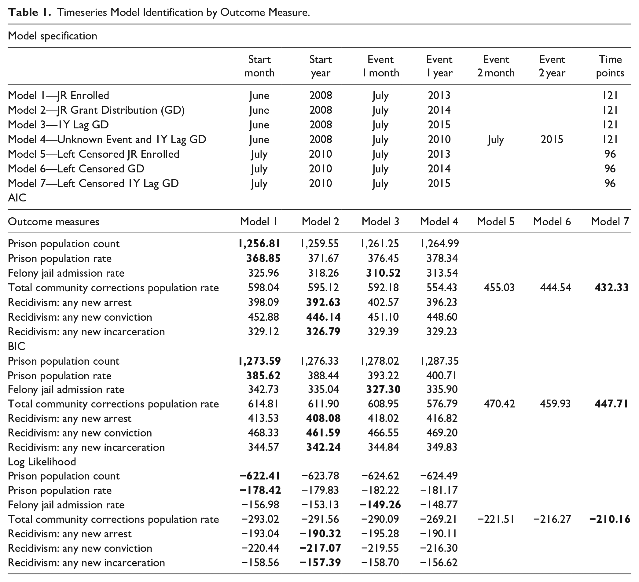
Model 1 involves all variables (see Table 1) and is used as the baseline model. Model 2 was compared to Model 1 for fit. All metrics of model fit in Table 1 (AIC, BIC, and Log Likelihood) indicate Model 2 is a better fit for most time series with the exception of the two prison population variables. All recidivism variables are best modeled by Model 2 (see Table 1, Outcome Measures) which models the direct effect of the distribution of grant funds to jurisdictions. Visual inspection of the felony jail admissions regression suggests this is still not the best fit. Table 1 reflects this assessment, where Model 3 improves model fit for two dependent variables—felony jail admissions and total community corrections population. The most notable issue with model fit was discovered upon visual inspection of the regression plot for total community corrections. This plot revealed a major trend change in the pre-justice reinvestment period and presented a substantial threat to the assumption of nonspuriousness and to the estimation of the historical (pre-event) trend.

In response to this issue, Model 4 was designed to represent the unknown event in July 2010 and the 1 year lagged effect of funding distribution in July 2015. Model 4 substantially increased fit for total community corrections but not for any other dependent variable. Furthermore, the regression coefficients for total community corrections (2010 event and JRA) were all significant, but the level and trend variables for the 2010 event were both nonsignificant for all other models. While Model 4 produced slight changes to the log likelihood values for the recidivism data, parsimony and the significance tests indicate that Model 2 is still the best fit for those data. The unknown event appears to be isolated to the community corrections population. However, the significant influence of the 2010 event on community corrections data must be addressed. Since this event occurs in the pre-period, retaining it in the regression equation would fundamentally alter the counterfactual.

To account for this event, and maintain the integrity of the counterfactual, the time series was left-censored in July 2010, leaving 96 timepoints for analysis. Truncating the data in this way absorbs the unknown event into the historical period prior to JRA’s enrollment. Models 5, 6, and 7 revisit the event structures of the first three models for the total community corrections dependent variable starting in 2010 rather than 2008. Model 7, the left censored 1 year lagged grant distribution (July 2015), provides the best fit for this dependent variable and the regression coefficients for the events did not change substantially after the left-censoring of the data (between Models 1 and 5, 2 and 6, and 3 and 7). The best fit for each model, as designated by the lowest value, is bolded in Table 1. These are the models analyzed below. To summarize, prison population variables (rates and counts) are best modeled by Model 1. All recidivism variables are best modeled by Model 2: No other model produces substantial changes between model fit values. Model 3 best fits the structure of felony jail admissions. Finally, community corrections populations are best modeled by Model 7, the left censored 2015 event structure.

ARIMA Fit

Table 2 reports the ARIMA model goodness of fit (represented by the Q and p values) and parameter estimates (i.e., autoregressive, moving average, and seasonal parameters). Significant Q values (i.e., p < .05) indicate statistical difference from random noise; there is still autocorrelation in the model. Therefore, iterating until the null hypothesis can be accepted (i.e., residual is not different from noise) is required to ensure that autocorrelation has been cleaned from the series. Table 2 shows that all models produced Q values that were not statistically significant at the .05 level, meaning that autocorrelation was sufficiently removed. Additionally, ARIMA model parameter estimates must all be statistically significant when reducing autocorrelation in the time series. Table 2 also shows that all models have statistically significant parameters that, taken together with the Q statistic, indicates each ARIMA model has successfully “cleaned” all autocorrelation from the data.

Table 2.

ARIMA Model Parameter Estimates and Q Fit.

Dependent series	(ARIMA)	Q (df)	p		Est. (SE)	Z
Prison count	(1,0,0) (1,0,0)12	21.42 (25)	.67	ar 1 =	0.99 (0.01)	193.53***
Prison count	(1,0,0) (1,0,0)12	21.42 (25)	.67	sar 1 =	0.31 (0.09)	3.24**
Prison rate	(1,0,0) (1,0,0)12	22.56 (25)	.60	ar 1 =	0.96 (0.02)	43.65***
Prison rate	(1,0,0) (1,0,0)12	22.56 (25)	.60	sar 1 =	0.29 (0.09)	3.11**
Felony jail adm rate	(0,1,1) (0,0,1)12	29.80 (25)	.23	ma 1 =	−0.73 (0.07)	−11.12***
Felony jail adm rate	(0,1,1) (0,0,1)12	29.80 (25)	.23	sma 1 =	0.26 (0.10)	2.58**
Comm. superv. rate	(1,1,0) (0,0,0)0	24.64 (25)	.48	ar 1 =	0.37 (0.09)	3.94***
Rearrest rate	(0,1,1) (0,0,0)0	22.36 (25)	.61	ma 1 =	−0.63 (0.11)	−5.64***
Reconviction rate	(0,1,1) (0,0,0)0	13.92 (25)	.96	ma 1 =	−0.35 (0.13)	−2.81**
Reincarceration rate	(0,1,1) (0,0,0)0	15.65 (25)	.92	ma 1 =	−0.59 (0.11)	−5.23***

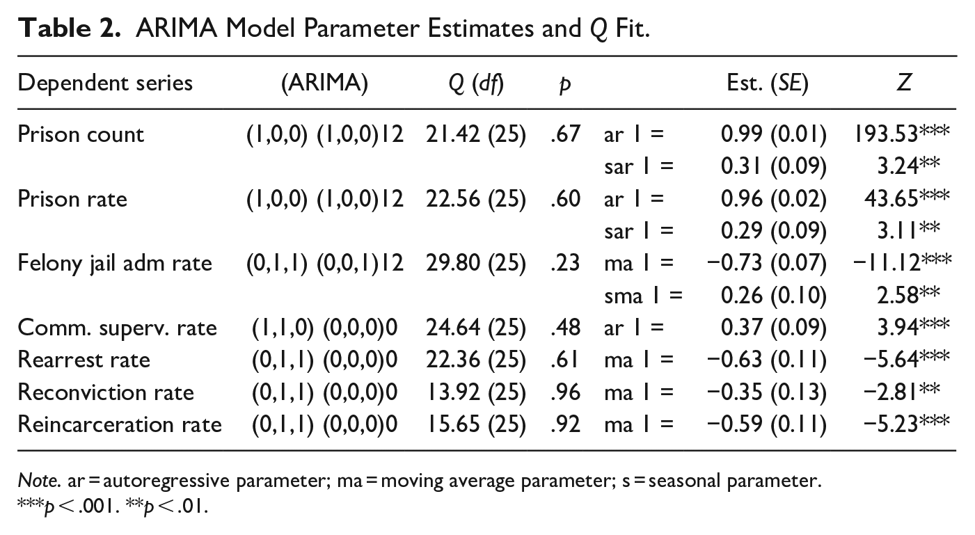
Note. ar = autoregressive parameter; ma = moving average parameter; s = seasonal parameter.

***

p < .001. **p < .01.

Results

GLS Regression

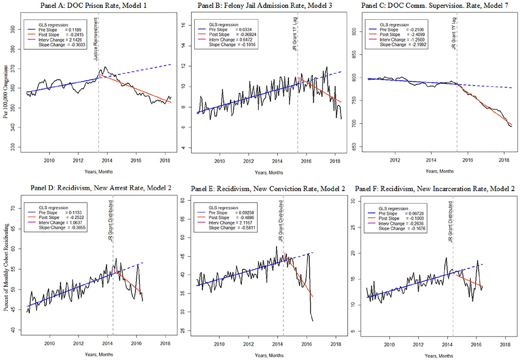
The regression coefficients, comparative fit indices, and change values for each of the seven ITS analyses, plotted in Figure 2 Panels A through F, are in Table 3. The intercept and time estimates model the pre-JRI starting level (intercept) and change (unit increase per month). These are not highlighted for statistical interpretation as they represent the starting point of the ITS regression, which provides the level and trend regression coefficients. Level indicates change immediately after the JRA passage, and trend models the post-JRA slope which may be significantly different from the pre-intervention slope. Finally, for each of the seven analyses the absolute and relative change observed by the end of the study period are provided. The absolute change indicates the raw value difference between the counterfactual period and the estimated post-JRI regression line, and the relative change converts this number into a percent.

Table 3.

Regression Coefficients and Absolute and Relative Change.

	A	Prison pop. count (1, 0)			B	Prison pop. rate (1, 0)
		2008–6, 2013–7, 2018–6				2008–6, 2013–7, 2018–6
		Est.	SE	t -Value		Est.	SE	t -Value
Regression coefficients	Intercept	13,585.97	−69.99	194.10		357.83	−1.92	186.48
	Time	13.24	−1.74	7.63		0.12	−0.05	2.51
	Level	89.45	−42.2	2.12*		2.14	−1.1	1.99*
	Trend	−7.04	−2.99	−2.35**		−0.36	−0.1	−4.40**
		Count				Rate
Change	Absolute	−333				−19.5
Change	Relative	−2.2%				−5.2%
	C	Felony jail adm. (0, 1)			D	Comm. superv. pop. rate (1, 0)
		2008–6, 2015–7, 2018–6				2010–7, 2015–7, 2018–6
		Est.	( SE )	t -Value		Est.	SE	t -Value
Regression coefficients	Intercept	7.43	−0.19	39.05		797.86	−3.53	225.98
	Time	0.03	0	8.70		−0.21	−0.09	−2.30
	Level	0.65	−0.35	1.85		−1.25	−2.25	−0.56
	Trend	−0.10	−0.01	–7.04***		–2.2	−0.2	−10.12***
		Rate		Count		Rate		Count
Change	Absolute	−3.0		−126		−80.4		−3,378
Change	Relative	−26.3%				−10.3%
	E	Any new arrest (0, 1)			F	Any new conviction (0,1)
		2008–6, 2014–7, 2016–6				2008–6, 2014–7, 2016–6
		Est.	( SE )	t -Value		Est.	SE	t -Value
Regression coefficients	Intercept	45.66	−0.51	90.36		36.98	−0.7	52.82
	Time	0.11	−0.01	9.56		0.09	−0.02	5.65
	Level	1.06	−1.01	1.06		2.12	−1.38	1.53
	Trend	−0.37	−0.06	−5.79**		−0.58	−0.1	−6.67***
		Percent (%)				Percent (%)
Change	Absolute	−7.7				−11.8
Change	Relative	−13.6				−25.7
	G	Any new incarceration (0, 1)
		2008–6, 2014–7, 2016–6
		Est.	( SE )	t -Value
Regression coefficients	Intercept	11.36	−0.37	30.82
	Time	0.07	−0.01	7.78
	Level	−0.26	−0.73	−0.36
	Trend	−0.17	−0.05	−3.65***
		Percent (%)
Change	Absolute	−4.3
	Relative	−24.0

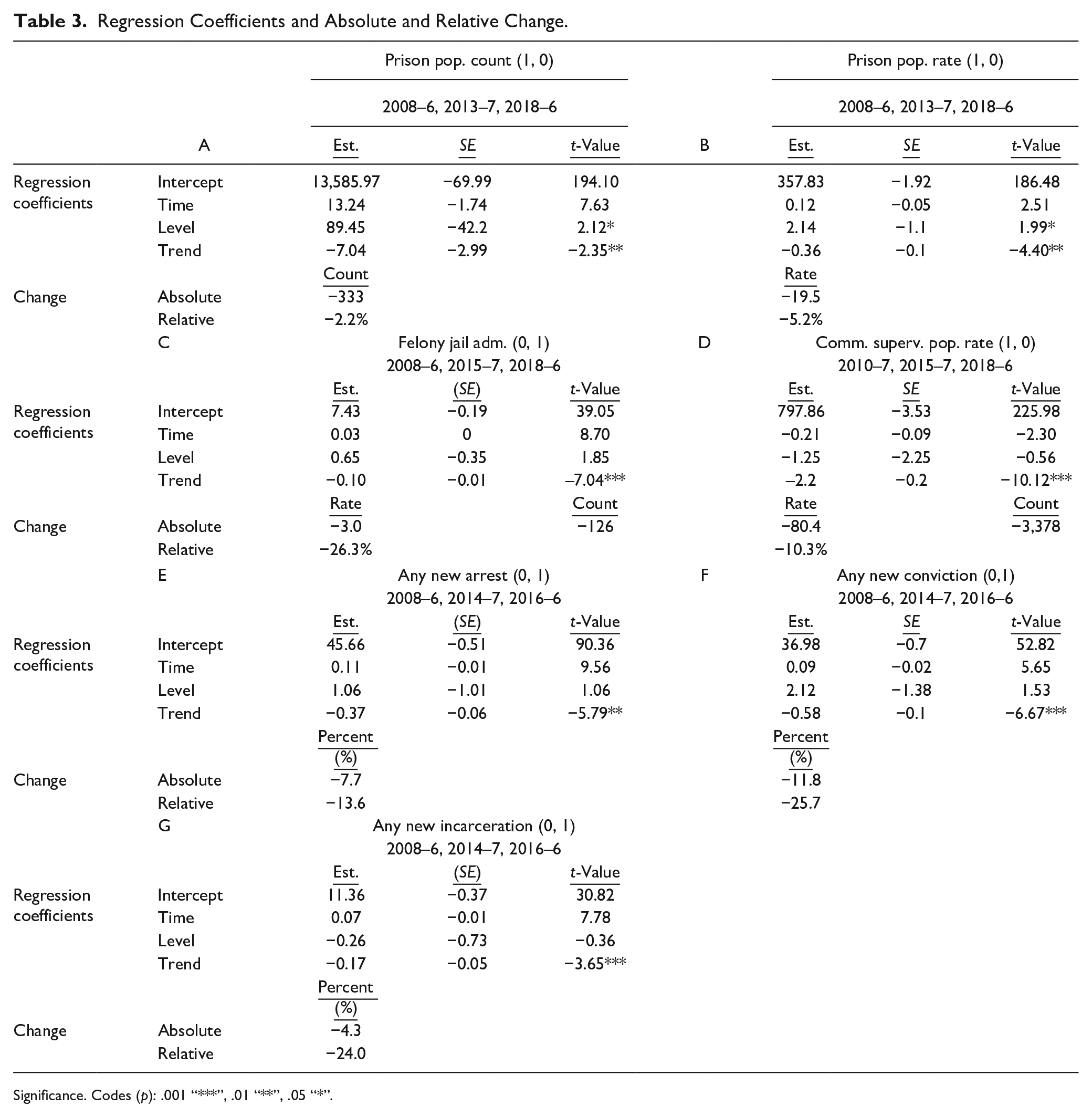
Significance. Codes (p): .001 “***”, .01 “**”, .05 “*”.

Prison population count

The state prison count was 13,586 prisoners at the start of the study period, June 2008 (Figure 1, Table 3 Panel A). Prior to the JRA, the number of people incarcerated in Oregon increased by about 13.24 prisoners per month. This regression line of best fit (trend) is shown as a solid blue line; and is projected into the post period as a dotted blue line, shown in Figure 1. This represents the counterfactual: An estimate of the pre-intervention prison population growth projected to the end of the study. The counterfactual line represents an estimated regression line of data that had continued throughout the study period as before. While this assumes a linear increase, it is a visual device by which to decipher a null hypothesis.

Figure 1.

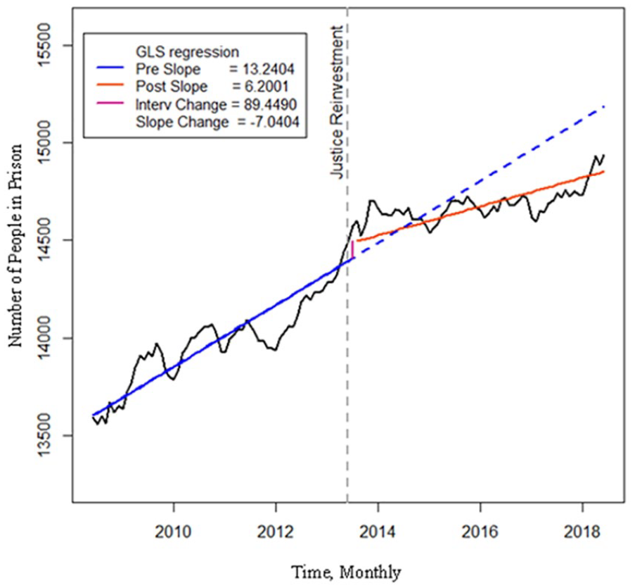
Oregon Justice Reinvestment: Prison population count, Model 1.

After the JRA was passed in July 2013, there was an immediate and significant (p = .036) step increase by an estimated 89 people. This is represented by the magnitude of solid purple vertical line at the intervention date. Following this slight increase, the rate of population growth significantly decreased by −7.04 people per month (p = .024), slowing to an estimated growth of six people per month after August 2013. The solid red line in Figure 1 is the regression line of best fit for the data in the post-period. Together, the slight immediate increase and the decreased rate of incarceration resulted in an estimated reduction of 330 fewer people in prison in June 2018. This means that after 59 months there were approximately 2.2% fewer people housed in Oregon’s prisons—compared to the counterfactual estimate in June 2018.

Prison population rate

The level of persons held in the state’s prisons per 100,000 Oregonians, shown in Panel A of Figure 2, was 358 prisoners in June 2008 (Figure 2 Panel A; Table 3 Panel B). The pre-intervention trend was approximately 0.12 new prisoners per 100,000 people per month. As in the count data, after July 2013 there was a significant (p = .049) and immediate step increase of 2.14 prisoners per 100,000 in August 2013. However, this was short-lived; there was a net trend change of −0.36 prisoners per 100,000 per month (p < .001). The post-intervention trend represents a decrease of roughly −0.24 prisoners per 100,000 per month. Ultimately, the absolute change in prison rate was roughly 20 fewer people per 100,000 in prison between the regression estimate and the counterfactual estimate for June 2018. After 59 months, the significant trend change translated to approximately 5% fewer people in Oregon’s prisons per 100,000 citizens than had the prison population rate stayed the same.

Figure 2.

Oregon Justice Reinvestment outcomes.

Felony jail admissions rate

Beginning at 7.43 admissions per 100,000 Oregonians in June 2008, the pre-intervention felony jail admission rate increased by 0.03 admissions per 100,000 per month (Figure 2 Panel B; Table 3 Panel C). After August 2015, the level of jail admissions did not significantly change. There was a significant (p < .001) trend change of −0.10 people per 100,000 admitted to jail on felony charges per month. The time series remained unchanged until July 2015 (Panel B in Figure 2), when a significant decrease in felony jail admissions occurs. The resulting post-intervention trend is −0.02 felony jail admissions per 100,000 per month, which equates to an absolute change of roughly three fewer people per 100,000 being admitted to jail on felony charges in June 2018. The significant trend change produces a relative total change of 18% fewer felony jail admissions in June 2018 when compared to the counterfactual. Inverting the population rate suggests that there were approximately 126 fewer people admitted to jail on felony charges in June 2018 when compared to the counterfactual.

Community supervision population rate

The aggregated community supervision level (Figure 2 Panel C; Table 3 Panel D) was estimated to be 798 individuals on either probation or post-prison supervision in July 2010. This decreased by an estimated 0.21 individuals per 100,000 each month until July 2015. The GLS regression found no statistically significant immediate level change. However, there is a significant decrease of 2.2 supervised individuals per 100,000 over the post-intervention period (p < .001). In addition to a slight decline from the pre-intervention period, this results in a steep decline of −2.41 individuals per 100,000 on community supervision after July 2015. The absolute difference between the regression and counterfactual estimates for June 2018 is a decrease of 80.4 per 100,000 people supervised by community corrections in Oregon: a reduction of approximately 10%. Inverting the population rate translates this change: If the trend of the pre-period had remained uninterrupted, we estimate there would have been 3,378 more people on community supervision in June of 2018.

Recidivism rates

Recidivism rates were partitioned by three specific criteria emphasized by the JRA: rearrest, reconviction, and reincarceration. Beginning with the June 2008 cohort, 45.66% of parolees recidivated by way of new arrest within 3 years (Figure 2 Panel D; Table 3 Panel E). This rate increased by approximately 0.11% for the remainder of the pre-intervention period. There was no significant immediate level change in August 2014; but a significant trend change was observed—a decrease of 0.37% per month (p < .001). After August 2015, each monthly cohorts’ rate of recidivism by new arrest decreased by −0.25% per month. This translates to an estimated decrease of 7.7% fewer people being rearrested in the June 2016 cohort which is a 13.6% relative decrease in the rate of recidivism by rearrest. These decreases are calculated in comparison to the counterfactual.

Similar, yet more pronounced, patterns were observed in reconviction (Figure 2 Panel E; Table 3 Panel F). Approximately 36.98% of the June 2008 release cohort was reconvicted (the intercept). For each subsequent release cohort, there was an increase of 0.09% more people receiving a new felony conviction per month. There was no significant level change estimated in the first month of the post-period (August 2015). There was a significant trend change between the pre- and post-periods of −0.58% (p < .001). Essentially, for every release cohort after August 2015, there was a reduction of −0.48% that recidivated by new felony conviction. This means that by the end of the study period, 11.8% fewer people had been convicted of a new felony than if the rate had remained unchanged. This represents a 25.7% decrease (relative change) in the rate of reconviction from what the estimated trend would have been, if the timeseries had not undergone significant change.

Recidivism by reincarceration (Figure 2 Panel F; Table 3 Panel G) also experienced significant changes. The June 2008 release cohort had a total reincarceration rate of 11.36%. This increased by 0.07% for every subsequent release cohort in the pre-intervention period. Modeling a 1 year lag from the enrollment of justice reinvestment (and coinciding with the distribution of funds) suggests there was no immediate level change, but a significant trend change of −0.17% (p < .001). After August 2015, the rate of recidivism by reincarceration decreased by 0.10% each subsequent month. Such a reduction translates to an estimated 4.3% fewer people being reincarcerated for the June 2016 cohort compared to the projected counterfactual for the same cohort (had the pre-period rate remained unchanged). When compared to the counterfactual, the 4.3% change equates to a 24% reduction from the estimated reincarceration rate for June 2016 had JRA not been implemented. Overall, this suggests that there were significant decreases in recidivism for people on community supervision (both probation and parole) after Justice Reinvestment funds were disbursed.

Discussion

Although many states are engaging in justice reinvestment efforts to reduce prison use and save costs, few empirical investigations have evaluated the aggregate impacts of JRI. This study provides an assessment of the effects of Oregon’s justice reinvestment legislation on rates related to imprisonment, felony jail admissions, community supervision populations, and recidivism in a quasi-experimental ITS design. The macro-level design is preferred for its comparability to existing research and because the sentencing changes affect the whole state equally. However, this design cannot evaluate the mechanism by which JRA is significantly associated with change (to do so would require a micro-level design). Our hypotheses were adopted from the legislative goals of justice reinvestment, which aimed to reduce prison use and recidivism. In addition, we incorporated other hypotheses to gage potential latent outcomes including felony jail admission rates and community corrections populations. Ultimately, our analyses revealed that the presence of the JRA was associated with a significant decrease in prison counts and rates immediately after being signed into law. These results are conglomerated into Table 4.

Table 4.

Results: Model Fit, Regression Estimation, and End of Series Change From Counterfactual.

Timeseries	Model fit	Historical behavior	Immediate impact	Trend change per month	Absolute change	Overall (relative) change (%)
Prison population (count)	Model 1	Increasing	+89.45*	−7.04**	−333 people	−2.2
Prison rate	Model 1	Increasing	+2.14*	−0.36**	−19.5^a	−5.2
Felony jail admit rate	Model 3	Increasing	NS	−0.10***	−3.0^a	−26.3
Community supervision rate	Model 7	Decreasing	NS	−2.20***	−80.4^a	−10.3
Recidivism—new arrest	Model 2	Increasing	NS	−0.37**	−7.7%	−13.6
Recidivism—new conviction	Model 2	Increasing	NS	−0.58***	−11.8%	−25.7
Recidivism—new incarceration	Model 2	Increasing	NS	−0.17***	−4.3%	−24.0

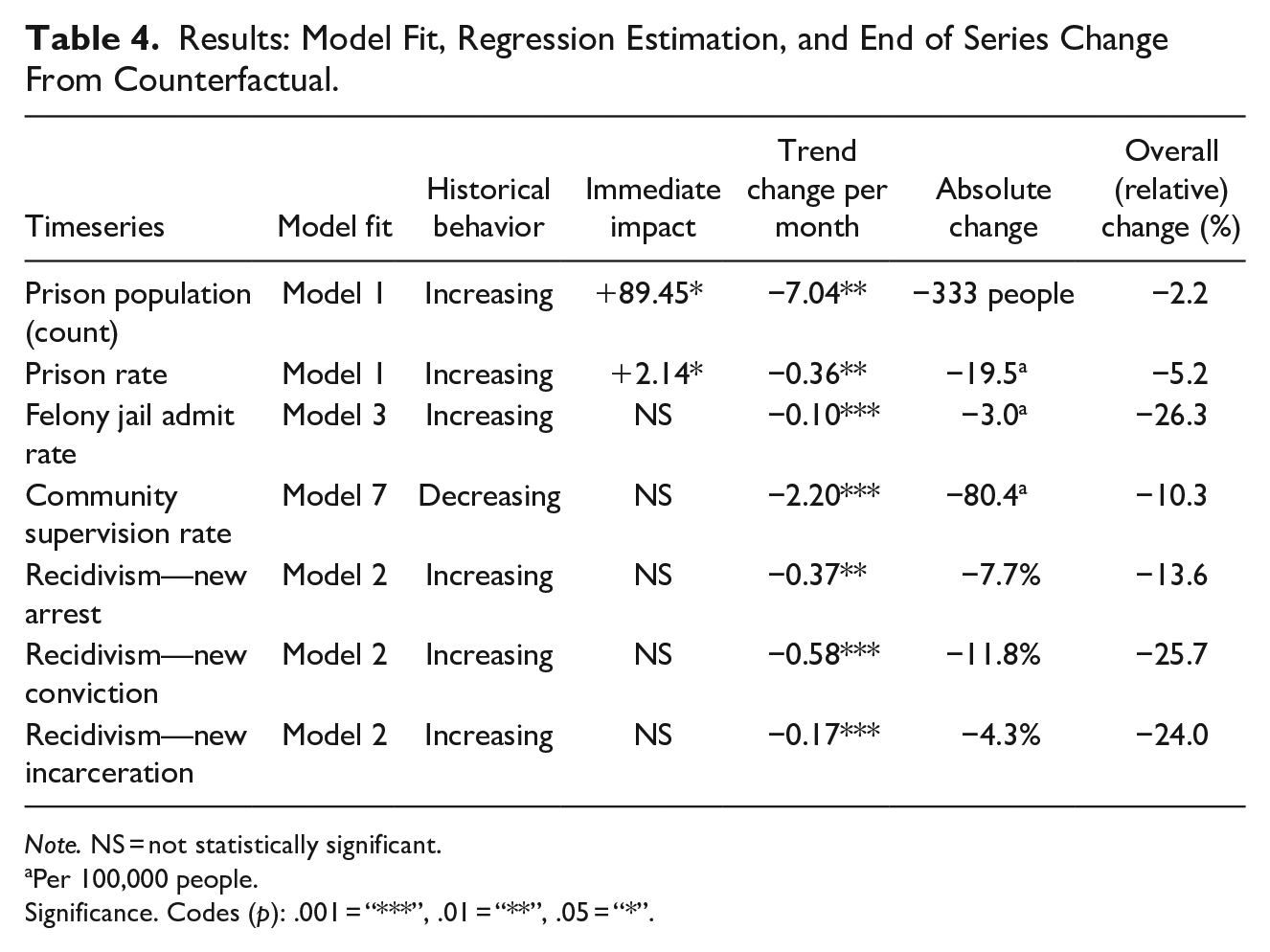
Note. NS = not statistically significant.

Per 100,000 people.

Significance. Codes (p): .001 = “***”, .01 = “**”, .05 = “*”.

The analysis of prison population rate per 100,000 Oregonians finds a full reversal in slope after justice reinvestment was passed in July 2013. Although there is likely some lag involved in this effect (the trend does not immediately begin to decline in August 2013) this suggests that the impact of the legislation may be very large, changing from a positive slope to a negative slope. However, comparison to the raw counts of individuals incarcerated in Oregon tells a different story: After August 2013, while the rate of increase for the count data slows significantly, it is still increasing—but in the population adjusted time series the post period rate steeply decreases. In fact, after the JRA was enrolled, the pace at which the monthly prison population count was increasing halved, from 13.24 to 6.20. This suggests that despite a continuously decreasing rate of decline for the prison rate per 100,000 this decline is not enough to stop the increase in prison usage in the state. Our analysis indicates that Oregon experienced a 2.2% reduction in prison use that is associated with the implementation of the JRA. Compared to the available analyses that examine Justice Reinvestment Initiative performance, Oregon appears to follow suit with those reporting a modest impact. In total, we find support for our first expectation; but understanding why the prison reduction appears stagnant will be critical to improving the yield of justice reinvestment in Oregon.

Our second and third expectations, that felony jail admission rates and community corrections populations would both increase, are not supported. The changes in these data may be explained by a 1 year lagged effect due to the delay in the distribution of grant funds to jurisdictions and are associated with significant decreases in the rate of felony jail admissions. Interpreting this result is nuanced. Immediately following the enrollment of the JRA, felony jail admissions continued to rise as expected and community corrections populations did not change substantially. However, it appears that programs funded by justice reinvestment within this period were slow to roll out, needing at least two full years to implement fully. After this period, a significant reduction in both felony jail admissions and the community corrections population did occur. An optimistic approach to understanding this effect is in conjunction with the outcomes of recidivism—where the programming works and reduces propensities for criminal justice involvement in supervised individuals. Therefore, people are exiting community supervision without revocation. However, this study cannot assess the validity of this, or any, interpretation of the cause for these changes.

It is possible and equally likely that there is a neutral explanation. For example, this result may indicate that judges and district attorneys are charging more felonies as misdemeanors in an effort to reduce prison use. These misdemeanors may involve diversion programs that also use less supervision. As prison-presumptive sentences divert more, nonviolent, moderate- and high-risk individuals to community supervision, low-risk individuals may be diverted away from probation entirely. This possibility is contained in reports from the Oregon District Attorneys Association (ODAA) which discusses efforts to identify alternatives to incarceration through diversion for JRI related offenses (see ODAA, 2018). A pessimistic interpretation might suggest that community corrections populations are decreasing because they are being revoked and sent back to prison. However, we find this unlikely because all three metrics of recidivism showed significant trend changes (from positive slopes to negative, decreasing, slopes). If this explanation were correct, we would expect reincarceration percentages to increase.

All three recidivism dependent variables have significant post-intervention negative trends which supports our fourth expectation that recidivism would decrease. The change in the data is best explained by a model that utilizes a 1 year lag from the enrollment of the JRA, coinciding with the first distribution of Justice Reinvestment Grant funds. It appears that as soon as the money began rolling out, recidivism by way of new arrests, convictions, and incarcerations stabilized then decreased. Cohorts that had access to resources (likely) supported by Justice Reinvestment funds for the entire 3 year follow-up period appear to not experience an increase in recidivism. Additionally, the more time that programs had to be implemented and strengthened, the more likely that release cohorts were to experience significantly lower recidivism rates across all three metrics. These changes are quite substantial. By 2016, the end of the most recently completed cohort, the state of Oregon exhibited overall reductions in recidivism of 13.6%, 25.7%, and 24% for rearrest, reconviction, and reincarceration, respectively. The spike in all three recidivism time series shortly after 2016 is curious and will require further investigation to explain. Contextually, this does not mean that more people were revoked in the early parts of 2016, but that the early 2016 release cohorts recidivated at higher percentages within 3 years downstream.

These trends provide evidence for the overall success in the reinvestment of funds into evidence-based community supervision practices. Such efforts are consistent with Taxman et al.’s (2014) call for states to adopt methods that research has shown to “work” in reducing recidivism when implementing JRIs. Compared to the limited existing research on JRI performance measures, these findings in Oregon appear to be on par with Pelletier et al.’s (2017) findings and improving upon trends observed elsewhere (Idaho Department of Correction, 2019).

Limitations and Future Directions

As with all research, this study’s findings must be viewed within the context of its limitations. The scope of this study was limited by lack of access to financial data that reports how funds are spent. Lacking full implementation details from each jurisdiction also limits the explanations that can be suggested for the effects produced by JRA between local jurisdictions. Access to financial data would be a more accurate way to measure implementation of justice reinvestment and remains an area for future research.

As with many studies of JRI, there also exists a “black box” problem with the current investigation. Without process and implementation information, this study cannot say how or why JRI produced the effects that are seen in the analyses. Significant variance exists in programming implementation between jurisdictions. This could produce inconsistent effects on the measured populations within jurisdictions, which in turn would be masked by the macro, state level, analysis. Compounding the unknowns surrounding implementation, programs that are being funded may (or may not) have ensured high fidelity to each program’s theory or implementation process. Additionally, not all counties implemented their programs at the same time or with the same intensity. This could produce a lag in the start of the intervention between jurisdictions, which may influence the findings observed during the study period. Therefore, we recommend that future analyses include between- and within-jurisdiction differences in JRI implementation to unpack the “black box” of JRI. This specifically applies to states that release funding with few explicit downstream guidelines to specific jurisdictions in how to execute justice reinvestment. We acknowledge this as a crucial area of understanding that needs to be evaluated.

Further, confining the dependent variables to those explicitly stated in the JRA may limit a full analysis of the intervention. As Wright and Rosky (2011) suggest, added pressure could produce change in the system that may affect other microsystems not directly targeted or addressed by the law. For example, if more individuals are being released into community corrections and rehabilitation programs on parole or probation, logically it would follow that case numbers would rise for probation or parole officers unless more officers are hired. This added case load might, then, create additional stresses, which could translate to increased violations, remanding more people to custody, in order to decrease case load. While we do not find evidence of this phenomenon occurring in the present study, it may be present but undetected by our restricted choice of variables and resulting analysis. Different dependent variable types such as admissions, facility capacity, personnel caseloads, or average lengths of stay would possibly be more sensitive tests for collateral consequences of Justice Reinvestment.

Finally, there are two phases to the law’s implementation. The first is the restructuring of statutes that went into effect upon signing by the Governor. The second is the monetary allocation over a year later that actually funds the treatment and diversion programs for each jurisdiction. This may be better represented by a multiple intervention model that can parse out the individual effects of the JRA and the interaction of the two parts. We suggest this would be a fruitful avenue for future research.

Although the extent of the effects of the justice reinvestment policy are only observed here through early 2020—prior to the changes due to COVID-19—there are several aspects to be gleamed from this observation period; any attempts to extend the analysis of the JRA beyond 2019 will be complicated by responses to the COVID-19 pandemic. However, this study provides a valuable baseline with which to parse the co-mingled effects of JRA and the emergency response to the pandemic. With the effects discussed in this study, there is a possibility that some new reforms enacted after the COVID-19 changes might enhance the effects of JRA and may even produce greater reductions in prison use and recidivism. We argue that while there are important limitations to interpreting the effects of JRIs in Oregon, they do not minimize our study findings. These limitations may influence the variables but are unlikely to have enough effect to change the significance of the results. The quality and quantity of the data used here provide a robust picture of trends in each outcome investigated, despite the limitations. The use of 60 pre-intervention time points in our ITS analyses provides a strong baseline for the construction of our counterfactuals to make comparisons over time.

Conclusion

This study finds that justice reinvestment in Oregon is associated with a decrease in prison use and reducing recidivism. It provides insight to a number of research and policy issues. An inherent difficulty in justice reinvestment initiatives are the many approaches to implementation. These numerous strategies of implementation can occur both between and within states despite having the same goals such as reducing prison costs or reinvesting monies into efforts to decrease recidivism. Even with the necessary data and cooperation, measurement of effects can be difficult because an affected jurisdiction may be embedded within another jurisdiction, or within a state, that is not a JRI participant. This problem is not unprecedented; similar difficulties have existed in other areas involving alternatives to incarceration or intermediate sanctions (e.g., Morris & Tonry, 1990). Future research will benefit from utilizing raw counts and population adjusted variables so that absolute results may be available to legislators yet be compared to differing jurisdictions.

If a JRI effort is effective in its ability to reduce prison use, and incarceration overall, the averted savings could help provide resources to fund additional programs that reduce the load on the criminal justice system. However, it is currently unclear where generated savings or averted costs are actually being spent. Critical to any analysis of justice reinvestment is the ability to track how reinvestment funds are spent, what savings are achieved, and where those savings are allocated. All aspects of reinvestment funds must be traceable so that any improvements or detriments can be attributed to justice reinvestment as outcomes.

As noted by Tucker and Cadora (2003), technical assistance is only one of four areas of justice reinvestment; it does not alone represent the broader concept of reinvestment. Redirecting funds from prison use to local criminal justice efforts is a continued investment in the larger criminal justice system. However, reinvestment implies the intentional and specific transfer of funds from the larger criminal justice system to other social services such as mental health care, public education, and community development as crime prevention tactics. Since technical assistance represents short-term gains, the other broad areas that comprise reinvestment are needed to sustain systemic shifts of decarceration. Research has long highlighted the major causes and correlates of crime are associated with larger social issues, such as education, poverty, and unemployment. The technical assistance approach is not designed to address these issues. Justice reinvestment in technical assistance and the pursuit of short-term savings may help kickstart a larger shift toward public safety if more resources are ultimately invested in the agencies that can address such factors.

In this study, we find that the technical approach to justice reinvestment enacted by the State of Oregon has produced moderate decreases in prison populations. But there is more work to be done: The prison population rate of growth was halved, not fully abated. Reinvestment into efforts to reduce recidivism and prison usage are likely helpful, but it will only address part of the revolving-door problems in punishment and corrections. Without further direct investment in communities and social systems, there is little evidence to suggest that “Technical Assistance Justice Reinvestment” can reverse the powerful trends of mass incarceration on its own.

Footnotes

Appendix

Declaration of Conflicting Interests

The author(s) declared no potential conflicts of interest with respect to the research, authorship, and/or publication of this article.

Funding

The author(s) received no financial support for the research, authorship, and/or publication of this article.

ORCID iDs

Christopher W. Dollar

Christopher M. Campbell

Notes

Author Biographies

Christopher W. Dollar is a Doctoral Candidate in the Department of Criminal Justice and Criminology at Washington State University. His research interests include criminal justice policy, community and institutional corrections, rehabilitation and reentry, application of law, and comparative criminology. He has also worked as a Research and Evaluations Analyst for the Multnomah County (Portland, OR) District Attorney.

Christopher M. Campbell, PhD, is an Associate Professor in the Department of Criminology and Criminal Justice at Portland State University. His research interests include pretrial detention and supervision, institutional and community corrections, offender rehabilitation and reentry, and the application of criminological theory. He also works as a consultant for the U.S. Department of Justice, state legislatures, and departments of correction for evaluation research and to determine best practices. His recent work has appeared in Criminal Justice and Behavior, Criminology and Public Policy, Justice Quarterly, and Criminal Justice Policy Review.

Ryan M. Labrecque, PhD, is an Assistant Professor in the Department of Criminal Justice at the University of Central Florida. His research focuses on the evaluation of correctional interventions, the effects of prison life, the development of risk and needs assessments for community and institutional corrections settings, and the transfer of knowledge to practitioners and policy makers. His work has appeared in Crime and Delinquency; Criminal Justice and Behavior; Journal of Criminal Justice; Psychology, Public Policy, and Law; and Criminal Justice Policy Review.

References

American Civil Liberties Union Foundation. (2015). Overcrowding and overuse of imprisonment in the United States American Civil Liberties Union (ACLU). Office of the High Commissioner for Human Rights.

Austin

Cadora

Clear

T. R.

Dansky

Greene

Gupta

Young

M. C.

(2013). Ending mass incarceration: Charting a new justice reinvestment. The Sentencing Project.

Austin

Coventry

(2014). A critical analysis of justice reinvestment in the United States and Australia. Victims & Offenders, 9(1), 126–148.

Berry

W. D.

Lewis-Beck

M. S.

(Eds.). (1986). New tools for social scientists: Advances and applications in research methods. SAGE Publications, Inc.

Bureau of Justice Assistance. (2014). Justice Reinvestment Initiative State Assessment Report. Bureau of Justice Assistance.

Campbell

C. M.

Labrecque

R. M.

Weinerman

Sanchagrin

(2020). Gauging detention dosage: Assessing the impact of pretrial detention on sentencing outcomes using propensity score modeling. Criminal Justice Journal, 70, 101719.

Campbell

D. T.

Stanley

J. C.

(1963). Experimental and quasi-experimental designs for research. Houghton Mifflin Company.

Carson

A. E.

(2020). Prisoners in 2018 (Bulletin NCJ 253516). Bureau of Justice Statistics.

Clear

T. R.

(2011). A private-sector, incentives-based model for justice reinvestment: Justice Reinvestment. Criminology & Public Policy, 10(3), 585–608.

10.

Council of State Governments. (2017a). Justice reinvestment: Connecticut overview. Council of State Governments.

11.

Council of State Governments Justice Center. (2017b). Capitol Hill briefing highlights three states’ reductions in prison costs and reinvestments in public safety. Council of State Governments Justice Center.

12.

de Vocht

McQuire

Brennan

Egan

Angus

Kaner

Beard

Brown

De Angelis

Carter

Murray

Dukes

Greenwood

Holden

Jago

Hickman

. (2020). Evaluating the causal impact of individual alcohol licensing decisions on local health and crime using natural experiments with synthetic controls. Addiction, 115(11), 2021–2031.

13.

Dollar

C. W.

(2018). Evaluating the effectiveness of justice reinvestment legislation in Oregon: Analyses of state and county implementation [Master’s thesis, Portland State University]. https://doi.org/10.15760/etd.6346

14.

Federal Bureau of Investigation. (2015). Offenses known to law enforcement by Metropolitan and Nonmetropolitan Counties, 2015. [Data set]. Uniform Crime Report. Federal Bureau of Investigation.

15.

Federal Bureau of Investigation. (2021). Crime in the United States by volume and rate per 100,000 inhabitants, 2000–2019. [Data set]. Uniform Crime Report. Federal Bureau of Investigation.

16.

Fox

(2016). Applied regression analysis and generalized linear models. SAGE Publications.

17.

Freeman

(2003). Can we close the revolving door? Recidivism vs. Employment of ex-offenders in the US. Urban Institute.

18.

Harrop

J. W.

Velicer

W. F.

(1985). A comparison of alternative approaches to the analysis of interrupted time-series. Multivariate Behavioral Research, 20(1), 27–44.

19.

Harvell

Welsh-Loveman

Love

Durnan

Eisenstat

Golian

Mohr

Pelletier

Samuels

Thomson

Ulle

La Vigne

(2016). Reforming sentencing and corrections policy: The experience of Justice Reinvestment Initiative States. The Justice Policy Center, Urban Institute.

20.

Idaho Department of Correction. (2019). Annual community gap analysis [Joint report to the legislature between the Idaho Department of Corrections and Idaho Department of Health and Welfare]. Idaho Department of Correction.

21.

Justice Reinvestment Act, House Bill 3194, Enrolled. (2013). Joint Committee on Public Safety, 77th Oregon Legislative Assembly.

22.

Kaeble

Cowhig

(2018). Correctional populations in the United States, 2016. Bureau of Justice Statistics.

23.

La Vigne

N. G.

Bieler

Cramer

Kotonias

Mayer

Samuels

. (2014). Justice reinvestment initiative state assessment report. Urban Institute.

24.

Mai

Subramanian

(2017). The price of prisons: Examining state spending trends, 2010-2015. Vera Institute of Justice.

25.

McCleary

McDowall

Bartos

B. J.

(2017). Design and analysis of time series experiments. Oxford University Press.

26.

McDowall

McCleary

Meidinger

Hay

R. A.

Jr. (1980). Interrupted time-series analysis (Vol. 21). SAGE.

27.

Morris

Tonry

M. H.

(1990). Between prison and probation: Intermediate punishments in a rational sentencing system. Oxford University Press.

28.

Oleson

J. C.

Lowenkamp

C. T.

Cadigan

T. P.

VanNostrand

Wooldredge

(2016). The effect of pretrial detention on sentencing in two federal districts. Justice Quarterly, 33(6), 1103–1122.

29.

Oregon Criminal Justice Commission. (2018). History of Oregon’s justice reinvestment initiative. Oregon Criminal Justice Commission.

30.

Oregon Department of Corrections. (2019). Oregon offender population: Population trends. Oregon Criminal Justice Commission.

31.

Oregon District Attorneys Association. (2018). The Oregon criminal justice system: A continuing success story. Oregon District Attorneys Association.

32.

Oregon Measure 57, Senate Bill 1087, Enrolled. (2008). Special Session, 74th Oregon Legislative Assembly.

33.

Oregon Task Force on Public Safety. (2016). Justice reinvestment report to the legislature, October 2016. Oregon Criminal Justice Commission.

34.

Orrick

E. A.

Vieraitis

L. M.

(2015). The cost of incarceration in Texas: Estimating the benefits of reducing the prison population. American Journal of Criminal Justice, 40(2), 399–415.

35.

Ostrom

C. W.

(1990). Time series analysis: Regression techniques (Vol. 9). SAGE Publications, Inc.

36.

Pelletier

Peterson

King

(2017). Assessing the impact of South Carolina’s parole and probation reforms: Justice Reinvestment Initiative. The Urban Institute: Justice Policy Center.

37.

Petrich

D. M.

Pratt

T. C.

Jonson

C. L.

Cullen

F. T.

(2021). Custodial Sanctions and Reoffending: A Meta-Analytic Review. Crime and Justice, 50(1), 000–000.

38.

Pew Charitable Trusts. (2018). 35 states reform criminal justice policies through justice reinvestment: Legislative action aims to increase public safety return on corrections spending. Pew Charitable Trusts.

39.

Pinheiro

Bates

DebRoy

Sarkar

; R Core Team. (2018). nlme: Linear and nonlinear mixed effects models (Version 3.1-149) [R package version 3.1-131.1]. CRAN.

40.

Ramirez

J. R.

Crano

W. D.

(2003). Deterrence and incapacitation: An interrupted time-series analysis of California’s three-strikes law. Journal of Applied Social Psychology, 33(1), 110–144.

41.

R Core Team. (2020). R: A language and environment for statistical computing. R Foundation for Statistical Computing.

42.

Rydberg

Clark

(2016). Variation in the incarceration length-recidivism dose–response relationship. Criminal Justice Journal, 46, 118–128.

43.

Sabol

W. J.

Baumann

M. L.

(2020). Justice reinvestment: Vision and practice. Annual Review of Criminology, 3(1), 317–339.

44.

Schmidt

(2017). Cost avoidance report: Per House Bill 3194 (2013). Oregon Criminal Justice Commission.

45.

Schmidt

Officer

(2015). Justice reinvestment implementation in Oregon, August 2013 to April 2015. Oregon Criminal Justice Commission.

46.

Shumway

R. H.

Stoffer

D. S.

(2011). Time-series analysis and its applications. Springer.

47.

Sliva

S. M.

Plassmeyer

(2021). Effects of restorative justice pre-file diversion legislation on juvenile filing rates: An interrupted time-series analysis. Criminology & Public Policy, 20(1), 19–40.

48.

Taxman

F. S.

Pattavina

Caudy

(2014). Justice reinvestment in the United States: An empirical assessment of the potential impact of increased correctional programming on recidivism. Victims & Offenders, 9(1), 50–75.

49.

Tucker

Cadora

(2003). Justice reinvestment: To invest in public safety by reallocating justice dollars to refinance education, housing, healthcare, and jobs. Ideas for an Open Society, 3(3), 1–8.

50.

Underwood

Behunin

Lehman

King

Packer

(2020). A performance audit of the justice reinvestment initiative. Office of the Legislative Auditor General.

51.

U.S. Census Bureau. (2018). Annual estimates of the resident population for counties: April 1, 2010 to July 1, 2016: Oregon [Data set] United States Census Bureau.

52.

U.S. Census Bureau. (2021). Apportionment population and number of representatives by state: 2020 census. [Data set]. United States Census Bureau.

53.

U.S. Department of Justice. (2017). Prisoners and prisoner reentry. United States Department of Justice.

54.

White

M. D.

Dario

L. M.

Shjarback

J. A.

(2019). Assessing dangerousness in policing: An analysis of officer deaths in the United States, 1970–2016. Criminology & Public Policy, 18(1), 11–35.

55.

Wright

K. A.

Rosky

J. W.

(2011). Too early is too soon. Criminology & Public Policy, 10(4), 881–908.

56.

Zeileis

Hothorn

(2002). Diagnostic checking in regression relationships. R News, 2(3), 7–10.

57.

Zhang

Wagner

A. K.

Ross-Degnan

(2011). Simulation-based power calculation for designing interrupted time series analyses of health policy interventions. Journal of Clinical Epidemiology, 64(11), 1252–1261.

Evaluating Oregon’s Justice Reinvestment Act: An Interrupted Time-Series Regression of State-Level Outcomes

Abstract

Keywords

Literature Review

Origins of Justice Reinvestment

Justice Reinvestment in Oregon

Current Study

Method

Data

The Intervention: Justice Reinvestment

Dependent Variables

Prison counts and rates

Felony jail admission rate

Community supervision rate

Recidivism rate

Analytical Plan

Identification of autocorrelation

Regression modeling

R packages

Model Specification

ARIMA Fit

Results

GLS Regression

Prison population count

Prison population rate

Felony jail admissions rate

Community supervision population rate

Recidivism rates

Discussion

Limitations and Future Directions

Conclusion

Footnotes

Appendix

Declaration of Conflicting Interests

Funding

ORCID iDs

Notes

Author Biographies

References