Sage Journals: Discover world-class research

Abstract

When studying corruption’s consequences for voter turnout, reverse causality hinders identification; corruption may affect turnout, but an engaged citizenry may also improve governance. However, because good instruments are hard to find, most studies do not adjust for the issue. Here, I surmount the endogeneity problem by predicting turnout among second generation Americans with the level of corruption in their ancestral country. The core intuition is that the best predictors of turnout—education, income, and civic duty—are endogenous to corruption, internationally mobile, and reproduced inter-generationally. Thus, corruption in one country can affect turnout among the American-born children of the country’s émigrés. However, because turnout in US elections does not affect corruption in the ancestral country, there is no threat of reverse causality. Estimating the model with data from the Current Population Survey and the Varieties of Democracy Project reveals a statistically robust, substantively sizable negative effect of corruption on turnout.

Keywords

corruption and patronage political economy elections public opinion voting behavior

Introduction

The core intent of democratic elections is to confront politicians with a trade-off: They can extract rents while in office or retain power at re-election, but they can’t do both. When democracy functions well, the argument goes, an engaged citizenry reelects good incumbents and throws out the “rascals,” thereby ensuring good governance (Adserà et al., 2003; Ferejohn, 1986; Fiorina, 1981; Key, 1966; Powell, 2000; Przeworski et al., 1999). However, such accountability presumes that corrupt incumbents do not so disillusion citizens that they disengage from political life altogether. When that presumption is false however, democracy can quickly become perverted in a vicious cycle, wherein bad officials reduce citizen engagement and participation, making holding office all the more appealing for corrupt types, who further alienate the public, and so on.¹

Given these stakes, it is no surprise that scholars have long tried to parse corruption’s consequences for citizen’s political participation. At present though, consensus remains elusive. While some scholars find political participation increasing with corruption, others assert that corruption causes turnout to decline, while still others find that any effect of corruption is context-conditional.² A variety of factors may explain the disparate results, but here, attention is given to the empirical problem confronting all studies in this tradition. If democratic theory is right that citizen engagement is essential for securing good governance, then the level of corruption in a country is endogenous to the degree of participation among its citizenry.³ Accounting for the reverse causality is imperative to identify corruption’s effects for political participation, yet much of the existing scholarship does not make the appropriate adjustments. Presumably, this is because of the notorious difficulty of finding suitable instruments for the problem. And though we sympathize with the challenge, the problem remains: Without appropriate adjustments for the reverse causality, we risk misunderstanding what corruption portends for civic engagement and political participation.⁴

This paper proposes a novel approach to the endogeneity problem. The strategy is to exploit the fact that the two most important predictors of an individual’s propensity to vote—socioeconomic status and feelings of civic duty—have three important properties: They are endogenous to corruption, internationally mobile, and reproduced inter-generationally within the family. Combined, these attributes allow us to treat the United States as the location of a natural experiment. The US is composed of individuals who migrated from countries located in vastly different corruption equilibria and whose premigratory experiences with corruption had profound consequences on their education attainment, income, accumulated wealth, and attitudes toward political engagement. Importantly, education, wealth, and political dispositions are internationally mobile—either because they are embodied in the individual (e.g., education and political dispositions), or because of global economic integration (e.g., one’s wealth and potentially one’s income). Migrants therefore bring with them to the US their stocks of education, wealth, and civic duty. Furthermore, those attributes are passed along to the migrants’ American-born children, thus affecting the latter’s propensity to participate in US elections.

Leveraging this intuition offers a way to identify corruption’s effect, namely, by regressing the turnout decisions of second generation Americans on the level of corruption in their country of ancestry. Such a model can avoid the reverse causality that hampers existing research for a straightforward reason: International mobility and inter-generational transmission of SES and political attitudes allows corruption in source country i to affect the behavior of second generation Americans, but turnout in US elections is not expected to affect corruption in the ancestral country because US legislators have no policymaking authority in the ancestral country. By design then, causality can only flow from corruption to turnout—eliminating reverse causality and allowing identification of corruption’s effect.

I implement this design by combining turnout data from the U.S. Current Population Survey (Flood et al., 2020) with corruption data from the Varieties of Democracy project (Coppedge et al., 2021). The results show a substantively large and statistically reliable negative effect of corruption on voter turnout. Various robustness checks ensure that the result is not confounded by source country characteristics such as regime type or per capita GDP, nor some unmeasured country-specific confound that individuals with similar ancestry may share, say, political culture, political history, political institutions, or social structure. The result continues to hold when estimating multilevel models that cross-classify respondents according to their ancestral country and the US state and metropolitan area in which they live, to adjust for the fact that immigrant communities often settle disproportionately in particular areas of the country (Bartel, 1989) and that these areas differ in the obstacles and incentives they present to prospective voters (Cho et al., 2006).

These results confirm several existing studies (McCann & Domínguez, 1998; Stockemer, 2013; Sundström & Stockemer, 2015), contradict others (Inman & Andrews, 2015; Lacombe et al., 2016; Stockemer, 2013), and bolster the former set by showing that they are robust to reverse causality adjustments. But though these results are important in their own right, this paper also hopes to make a contribution to the theory regarding why corruption might exert this effect. As Brady et al. (1995) put it, there are three reasons why someone doesn’t vote: they can’t, they don’t want to, or nobody asked (p. 271). Notably, while there is no shortage of research linking corruption to turnout via the second and third pathways, no research highlights the first. The absence is puzzling. Not only is it well-established that political participation requires resources like education and income (Brady et al., 1995; Verba & Nie, 1972; Verba et al., 1978), it is also clear that corruption determines whether individuals can acquire those resources (Chua, 1999, 2000a; 2000b; Hicken and Simmons, 2008; Ferraz et al., 2012; Suryadarma. 2012; Duerrenberger & Warning, 2018; Mo, 2001; Gupta et al.,2002; Mauro, 1995; Gründler & Potrafke, 2019). These two stylized facts imply that along with the mechanisms highlighted in existing scholarship, corruption may also reduce turnout through its effects on SES. After presenting the main results summarized above, I investigate whether this pathway has empirical support by regressing the schooling attainment and family income of second generation Americans on the level of corruption in the ancestral country. Both dependent variables are decreasing with source country corruption suggesting that corruption may indeed reduce turnout through its effects on SES.

In spirit, this study is most similar to that from Chong et al. (2015) in that both seek to identify the causal effect of corruption on turnout. However, whereas Chong et al. (2015) use experimental manipulations in Mexico as the identification strategy, the present study seeks to draw leverage from enormous cross-national variation in corruption levels by exploiting the “natural experiment” implied in the notion of the United States as “a nation of immigrants.” It is telling that this study and Chong et al. (2015), though distinct in their research designs, arrive at similar conclusions regarding the consequences of corruption. This paper also belongs to a large literature documenting how source country attributes affect individual behavior. For instance, several studies use source country characteristics to identify the effect of culture on women’s fertility choices and labor force participation and on the household division of labor (Antecol, 2000; Blau et al., 2011; Fernández & Fogli, 2009; Giuliano, 2007). Borjas (1993) shows that the economic success of U.S. immigrants is predicted by source country characteristics. Meanwhile, political science research has also established that migrants’ premigratory experiences affect postmigratory political attitudes and behaviors (Bueker, 2005; Cho, 1999; Finseraas et al., 2020; Wals, 2011, 2013; Wals & Rudolph, 2018). None of these studies have highlighted the particular role of corruption though, making the present study a useful addition. Among studies that use such research designs to study corruption (e.g., Fisman & Miguel, 2007; Simpser, 2020), the goal has been to assess whether a culture of corruption exists, rather than addressing corruption’s behavioral implications for citizens.

The rest of this paper proceeds as follows. Below, I briefly review the relevant literature on corruption and voter turnout. Subsequent sections elaborate on the intuition of the empirical strategy, discuss the data and estimation, present the main results and robustness checks, and assess the validity of the novel SES pathway. Then, I conclude.

Surveying the Literature

There is no shortage of scholarship on corruption’s political repercussions. Early research insisted that corruption can be a boon for citizen engagement. For example, Huntington (1968, p. 64) famously argued that corruption can increase engagement by granting access to the state to those alienated from their government and excluded from political life. Likewise, Waterbury (1973) writes that “corruption permits access to the distribution system to groups and minorities that might otherwise be frozen out” (p. 542).

While recent research has discarded these specific arguments, two separate hypotheses concur that turnout is indeed increasing with corruption. The first maintains that as a violation of the social contract, corruption enrages citizens and motivates them to go the polls to install an opposition who will rehabilitate that contract (Inman & Andrews, 2015; Kostadinova, 2009; Stockemer & Calca, 2013). Kostadinova (2009) summarizes the argument well, writing that, “Revelations of secret deals struck by government officials to enrich themselves or the party coffers create incentives for some voters, who would otherwise choose to abstain, to vote the betrayers of public trust out of power” (p. 696). The second argument avers that an environment of pervasive corruption encourages “turnout buying” wherein incumbents offer selective incentives to their supporters who show up at the polls (Escaleras et al., 2012; Karahan et al., 2006; Lacombe et al., 2016).⁵

Despite these arguments, the more common expectation in contemporary scholarship is that corruption decreases voter turnout, though here again, explanations differ for why this might be so. One hypothesis is that citizens will see no benefit to voting when the supply of public policy is determined by bribery, extortion, and embezzlement, rather than vote shares (Caillier, 2010; Chong et al., 2015; Costas-Pérez, 2014; McCann & Domínguez, 1998; Stockemer, 2013; Stockemer et al., 2012; Warren, 2004). However, another counters that because turnout is more responsive to civic duty than to any material benefits that accrue from voting (Barry, 1970), the negative effect of corruption on turnout exists because public malfeasance weakens civic duty by causing citizens to see their government as illegitimate, undermining social and political trust, and otherwise alienating citizens from the state (Anderson & Tverdova, 2003; Bowler & Karp, 2004; Feitosa, 2020; Seligson, 2002; Stockemer, 2013; Sundström & Stockemer, 2015).

Given these various perspectives, it is not surprising that the evidence regarding corruption’s consequences for turnout is mixed. Several studies find evidence of a positive effect (Inman & Andrews, 2015; Kostadinova, 2009; Stockemer & Calca, 2013), though just as many report a negative one (Caillier, 2010; Chong et al., 2015; Feitosa, 2020; Giommoni, 2021; McCann & Domínguez, 1998; Stockemer, 2013; Sundström & Stockemer, 2015). Still others find no effect at all (Peters & Welch, 1980), or a context-conditional one (Bazurli & Portos, 2019; Costas-Pérez, 2014; Dahlberg & Solevid, 2016; Davis et al., 2004; Klašnja et al., 2016; Neshkova & Kalesnikaite, 2019; Školník, 2020). There are many potential causes for the disparate results. For example, scholars often diverge in what they talk about when they talk about corruption: some highlight perceptions, while others home in on experiences, scandals, or convictions. Likewise, the effect of corruption may differ depending on whether the country under scrutiny is rich, middle-income, or poor, or a consolidated democracy compared to a new one. The aim of the present study is to not adjudicate across all these potential explanations. Rather, I want to direct attention to the fact that looming large over the entire literature is the empirical problem of reverse causality. If the core premise of democracy is that good governance starts with an engaged citizenry that replaces bad incumbents with good ones (Adserà et al., 2003; Ferejohn, 1986; Fiorina, 1981; Key, 1966; Powell, 2000; Przeworski et al., 1999), then voter participation may determine corruption levels. Properly estimating corruption’s effects on turnout requires adjusting for this possibility, but most existing studies do not do so. The main difficulty with accounting for reverse causality would appear to be finding a good instrument. Below, I explain the intuition behind an alternative solution to the problem.

Intuition and Empirical Strategy

Start with the famous Riker and Ordeshook (1968) equation regarding the calculus of voting

R = p B - C + D,

(1)

where R represents the expected reward to voting, B are the benefits one accrues when one’s preferred candidate wins office, p is the probability of being the pivotal voter, C are the cost to voting, and D is the civic duty term. The core insight of the strategy is that some of the terms on the right-hand side of (1) have three important properties: They are endogenous to corruption, portable across international boundaries, and reproduced inter-generationally within the family. Combined, these properties allow identification of corruption’s causal effects.

To elaborate, start with the costs of voting that (1) encodes in the C term. Research has long shown that these costs are closely related to one’s stock of participatory resources. Education provides the cognitive skills that facilitate informing oneself about the politics of the day, for instance, while one’s income and accumulated wealth influence the ease with which one can navigate the bureaucratic hurdles to voting (Brady et al., 1995; Cho, 1999; Verba & Nie, 1972; Verba et al., 1978). Importantly, whether individuals acquire these resources depends on the level of corruption in a country. Consider corruption’s effect on education. Chua (1999; 2000a; 2000b) documents that corruption in the Philippines education bureaucracy has produced sizable kickbacks to politicians and bureaucrats but inadequate education to the country’s public school students. Likewise, Suryadarma (2012) shows that increases in public education spending in Indonesia only correlates with better enrollment outcomes in the less corrupt parts of the country. Ferraz et al. (2012) show similar evidence for Brazil. Duerrenberger and Warning (2018), Mo (2001), Gupta et al. (2002), and Hicken and Simmons (2008) generalize the point, finding in cross-national samples that higher levels of corruption are associated with lower levels of human capital accumulation. There is similarly strong evidence that corruption slows economic development and increases the poverty rate (Gründler & Potrafke, 2019; Gupta et al., 2002; Mauro, 1995; Mo, 2001).

Just as important as the endogeneity of SES to corruption is the fact that SES is internationally mobile. Because education is embodied in the individual, it necessarily crosses national borders at the same time an immigrant does.⁶ Likewise, in our current era of economic globalization, one’s accumulated wealth—and oftentimes, one’s income too—are mobile across international borders. Such mobility implies that the political consequences of corruption need not be bound by the national borders in which the corruption occurred. Rather, it can even affect the behavior or a country’s émigrés. To illustrate, consider two immigrants to the US from two separate countries, one who arrives in the US with sizable endowments in human capital and financial resources and the other with modest endowments in both. Though both individuals find themselves in an altogether new political landscape, the immigrant with the more abundant endowments might find it easier to navigate the US political terrain. She can use her sizable stock of education to acquire new knowledge about the political issues of the day and she can employ her accumulated wealth to overcome the bureaucratic hurdles to participating in US politics. All else constant, the more well-endowed immigrant is therefore expected to be more participatory in the US than her counterpart.

The same intuition applies to civic duty, the D term in (1) and probably the strongest predictor of the propensity to vote (Barry, 1970). Evidence abounds that civic duty declines with corruption because public malfeasance undermines regime legitimacy, lowers social trust, and otherwise reduces the utility of expressive voting (Anderson & Tverdova, 2003; Bowler & Karp, 2004; Feitosa, 2020; Seligson, 2002; Stockemer, 2013; Sundström & Stockemer, 2015). And like education, civic duty and political disaffection are dispositions embodied in individuals that cross national borders at same time an immigrant does. Wals (2011) provides the most direct evidence of this mobility, observing in a sample of Mexican immigrants in the United States that, “immigrants pack their prior political experiences and views in their political suitcase, later bringing them to bear when those immigrants encounter the American political arena” (p. 607).⁷

The international mobility of the SES and civic duty offer a way to avoid the reverse causality that hampers existing studies, namely, by predicting the turnout decisions of US immigrants in US elections with the level of corruption in their ancestral country. The advantages of the design are straightforward. The endogeneity of SES and civic duty to corruption and their international mobility mean that a country’s level of corruption can affect turnout among its émigrés in the US. However, turnout in US elections is not expected to have any effect on corruption in one’s ancestral country because the politicians elected in US elections have no policymaking authority in those other countries. Consequently, such a design allows corruption to affect turnout but not the reverse.⁸

Though free of reverse causality, studying immigrants in this way may exhibit another source of bias that hinders identification. Selection bias would be a problem to the extent that naturalized US citizens are different from their counterparts who do not undergo naturalization in ways correlated with the turnout decision. However, we can avoid this source of bias by taking advantage of the inter-generational transmissibility of SES and civic duty within the family. In more detail, scholars have long shown that parents’ political attitudes and behaviors are reproduced in their children (Jennings et al., 2009; Kudrnáč & Lyons, 2016; Plutzer, 2002; Verba et al., 2005). The reproduction is often purposeful and explicit, such as when parents teach their children the importance of voting and civic engagement (Jennings et al., 2009), though transmission also occurs indirectly when children observe their parents discussing the politics of the day (or not) and voting (or abstaining) on election day and come to internalize and emulate that behavior (Achen, 2002; Kudrnáč & Lyons, 2016; Plutzer, 2002; Tims, 1986; Valentino & Sears, 1998; Verba et al., 2005). Likewise, socioeconomic status is also reproduced in the next generation in the US (Borjas, 1993).

This inter-generational transmission means that a parent who, because of low socioeconomic status, declines to participate in electoral politics is likely to have a child less likely to do so for the same reason. Likewise, a parent who abstains from voting due to low civic duty is likely to have a child who exhibits a similar political disposition and similarly refrains from voting. Therefore, if corruption reduces SES and civic duty, corruption’s consequences can persist to affect the behavior of subsequent generations. Notice the key point though: Because all American-born children have birthright US citizenship, there is no naturalization process to introduce the selection effects that would exist in the study of their parents. Thus, combining the endogeneity of SES and civic duty to corruption with the international portability and inter-generational reproducibility of those attributes yields a strategy by which corruption’s effect on voter turnout can be identified, namely, by predicting the turnout decisions of second generation Americans with the level of corruption in their ancestral country.

Potential Criticisms of the Design

Before turning to the data to implement the strategy, two related critiques of it warrant attention. The first regards selection into immigration. Suppose that high-SES residents of a corrupt country are more likely to migrate to the United States than their low-SES compatriots because, say, the returns to their factors of production are higher in the US (Borjas, 1993), or because of the considerable resource requirements needed to migrate. If the selection process is strong enough, then the SES of US immigrants from corrupt countries (and their American-born offspring) will not differ much from that of immigrants from low-corruption countries. This would render the design unable to uncover corruption’s effect on turnout. A similar argument can be made with respect to civic duty.

The second critique regards inter-generational mean reversion. To simplify, let one’s wages, w, serve as shorthand for one’s socioeconomic status and following Borjas (1993), let w in country i be transmitted from generation t − 1 to generation t as follows: w_i,t = a_i,t + δw_i,t−1 + ϵ_i,t, where a is the average income in i and 0 < δ < 1. The notion of the United States as the “land of opportunity” implies a small δ and a strong regression to the mean across generations. But if δ is sufficiently small, then the SES of second generation Americans will be uncorrelated with the level of corruption in the ancestral country. This, too, would render the design unable to uncover any effect of corruption.⁹

Though we cannot rule out selection into immigration and mean reversion, it is important to note that the main effect of these processes is to make it harder to observe any effect of corruption on turnout. Figure 1 clarifies by showing the two pathways by which corruption can affect turnout in this design. First, corruption in source country j can affect the SES of the residents of j. Migrants from j bring their education and accumulated wealth with them to the US and transmit those attributes to their American-born children (denoted with the G2 superscript), thereby affecting the latter’s turnout decisions. Second, corruption can affect civic duty, which is similarly mobile internationally and reproduced inter-generationally. Notice that strong selection and mean reversion imply that variation in SES and civic duty among second generation Americans will be truncated, essentially holding constant the intermediate variables that transmit corruption’s effect. This makes it less likely to observe any effect of source country corruption on turnout in this design and means that any effects of corruption that are observed are likely to be conservative ones.

Figure 1.

Pathways by which corruption in the ancestral country might affect the turnout among second generation Americans.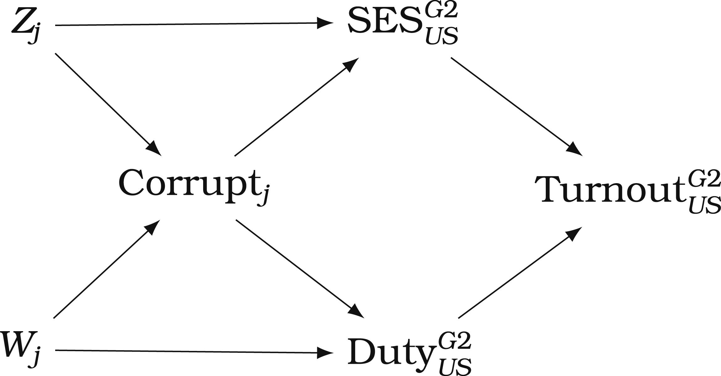

Data and Methods

Data on voter turnout data come from the Voting and Registration Supplement of the Current Population Survey for every presidential election between 2000 and 2016 inclusive (Flood et al., 2020).¹⁰ Second generation Americans are identified through items regarding the respondent’s country of birth and the birth place of the respondent’s mother and father. Because a second generation American may have parents who themselves were born in different countries, one must choose to associate the respondent with either the mother’s or father’s nationality. It is not obvious which parent to prefer, but it seems likely that inter-generational transmission of political attitudes and behavior is more successful when children receive consistent cues from their parents (Jennings et al., 2009). Accordingly, the main sample consists of second generation Americans where both parents were born in the same country. (Robustness checks presented below associate respondents with the mother and father ancestral countries separately and replicate the main results.)¹¹

The corruption data comes from the Varieties of Democracy Project (Coppedge et al., 2021), which codes six separate indicators of corruption and aggregates them into an index with an item response model.¹² An advantage of the V-Dem data over more commonly used alternatives like Transparency International’s Corruption Perceptions Index (CPI) or the measure from Political Risk Services’s International Country Risk Guide (ICRG) is the former’s longer time series. Whereas the CPI data start in 1995 (and are only comparable over time starting in 2012) and the ICRG begins in 1984, the V-Dem data start in 1900. The longer time series allows better matching of source country corruption to the time when the CPS respondent’s parents plausibly lived there (and absorbed the effects of corruption on civic duty and SES). To elaborate, consider that the parents of a 35 year old second generation American sampled in the 2016 CPS could have arrived in the United States as late as 1981, but neither the CPI nor ICRG have data going back that far. Using these data sources would therefore require imputing the source country corruption score from more recently available data, but this may be unreliable if the severity of corruption in the country changed over time. V-Dem’s longer time series allows us to use corruption data from the time the parent plausibly lived in the source country.¹³

The CPS conveys whether a respondent’s parents were born elsewhere, but it does not indicate the year they arrived in the United States, so it is not immediately evident how best to merge the CPS with the corruption data. One approach would be to apply a generic time frame—say, the average corruption score across the decade of the 1980s—to each respondent in the CPS. However, this presumes that respondents from the same ancestral country all receive the same “dose” of source country corruption, when this need not be the case. For example, according to the V-Dem data, India is considerably more corrupt today than it was in the 1950s and 1960s.¹⁴ Given such temporal variation, it is plausible that older respondents with Indian ancestry sampled in the 2016 CPS survey had parents who lived in India under very different levels of corruption than their 20-year old counterparts surveyed in the same election. Likewise, a 40 year old sampled in 2016 may have parents who experienced different levels of corruption while they lived in India compared to a similarly aged respondent sampled in 2000.

Such variation ought to be reflected when matching the corruption data to the CPS. To do so, I use the respondent’s age to demarcate a period of time during which it is plausible that the respondent’s parent lived in the source country. In particular, I construct a 10 year window, the last year of which is the respondent’s birth year, calculate the average V-Dem corruption score throughout that period, and use that respondent-specific average as the independent variable in the analyses below.¹⁵ The resulting measure captures well the variation in the dose of source country corruption among CPS respondents with similar ancestry. I demonstrate in Figure 2. As mentioned above, corruption has increased in India over time and that increase is reflected in Panel a of Figure 2. Meanwhile, Panel b plots the relationship between the respondent’s age and the dose of source country corruption received following the measurement strategy described above for the 240 second generation Americans with both maternal and paternal Indian ancestry in the sample. Consistent with what we surmised above, the respondent-specific average captures well the fact that for any given election year, older respondents with Indian ancestry were dosed with lower levels of source country corruption than younger voters were and for any given age, respondents sampled in more recent elections were dosed with more corruption than those sampled in the earlier ones.¹⁶

Figure 2.

Panel a: Corruption over time in India. Panel b: how the “dose” of source country corruption changes by age and election year among CPS respondents with Indian ancestry.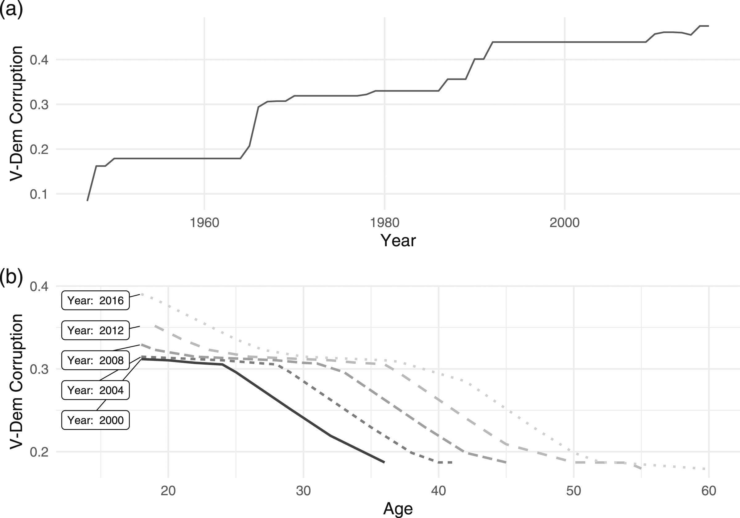

Control Variables

I estimate corruption’s effect with a logit model predicting a respondent’s decision to vote as a function of the level of corruption in their ancestral country. Such a model ought to account for several potential confounds. Recall, per Figure 1, that two pathways can transmit corruption’s effect in this design: SES and civic duty. Given these pathways, two kinds of factors need to be controlled for. First, we need to account for variables that correlate with both corruption and socioeconomic status—denoted Z_j in Figure 1. One such variable is the source country’s regime type; evidence shows that democracy correlates with corruption (McMann et al., 2019; Treisman, 2007) and with socioeconomic conditions (Baum & Lake, 2003). Another is the country’s per capita GDP. Secondly, we also need to control for factors that correlate with both corruption and civic duty—these variables are denoted as W_j in Figure 1—such as an element of the country’s culture like social trust (Almond and Verba, 1963; Mishler & Rose, 2005; Putnam et al., 1993) or some unobserved feature of the country’s social structure or political history.

To account for these confounds, I control for the source country’s regime type and its per capita GDP and I estimate the model in a multilevel framework that clusters respondents by their country of ancestry to account for unobserved confounds like culture, social structure, institutional environment, and history.¹⁷ The model also controls for the respondent’s sex and age. And since the sample includes data from all presidential election years between 2000 and 2016, the model also includes a dummy variable for each year, with 2000 being the excluded category. Lastly, though it is common in studies of voter turnout to control for the respondent’s education and income, in the present application, doing so produces post-treatment bias by blocking one of the pathways by which corruption might affect turnout. Such variables are therefore not included here. Table 1 displays the summary statistics for these right-hand side variables.

Table 1.

Summary Statistics.

		N	Mean	SD	Min	Max
	V-Dem Corruption	10796	0.51	0.30	0.00	0.96
	Polity	10796	−0.36	6.22	−10.00	10.00
	Per Capita GDP (logged)	10796	8.50	0.66	6.32	10.29
Sex	Male	5065
Sex	Female	5731
Age	18–29	3838
	30–39	1827
	40–49	1129
	50–59	712
	60–69	711
	70–79	1230
	80+	1349
Year	2000	1814
	2004	1877
	2008	1871
	2012	2573
	2016	2661

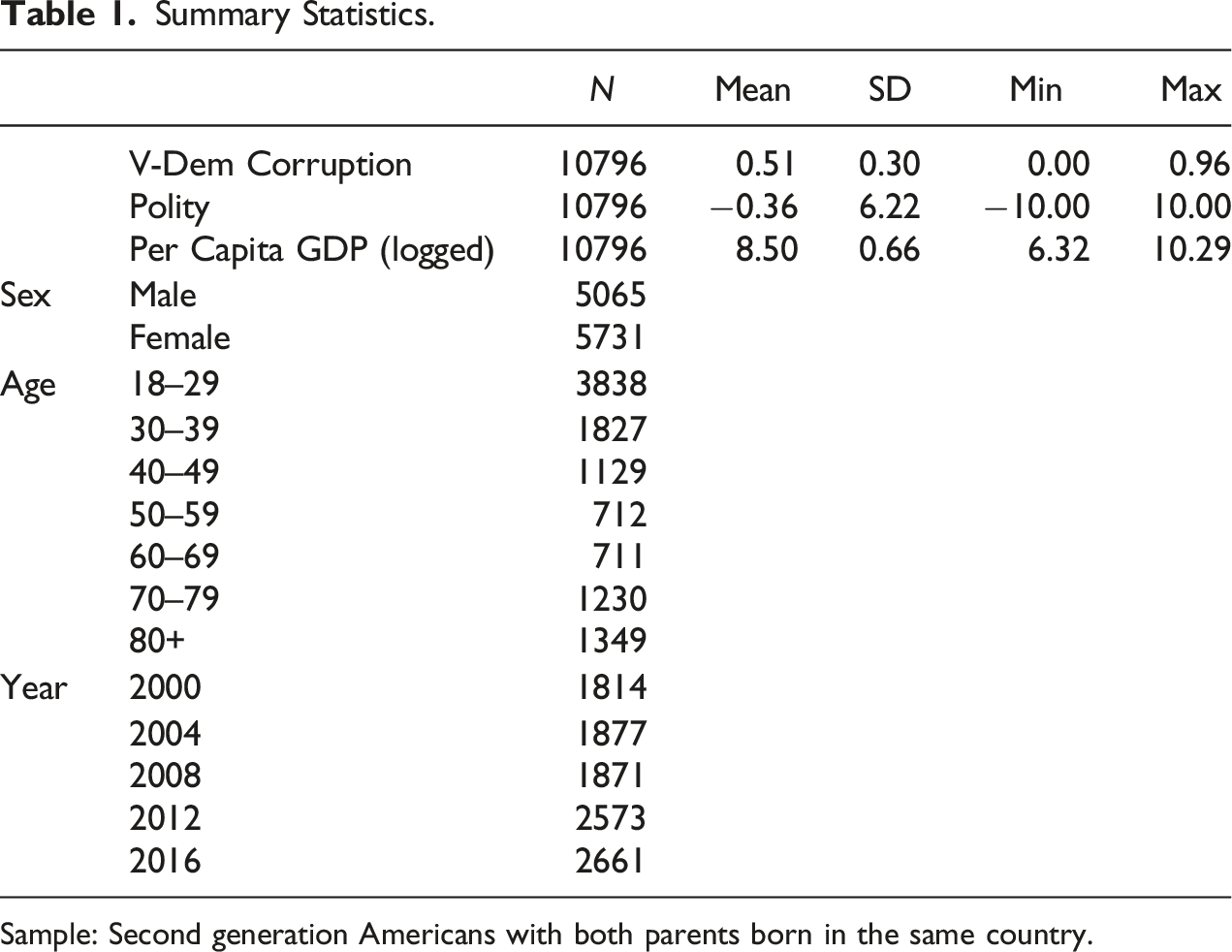
Sample: Second generation Americans with both parents born in the same country.

Estimation

The models are estimated in a Bayesian framework, which is preferred for the interpretation of estimation uncertainty and because such approaches can have benefits when estimating multilevel models (Gelman & Hill, 2007). Bayesian approaches necessarily require specifying prior distributions for the model’s parameters; however, the disparate results in existing scholarship noted in Section 2 do not enjoin one to assign especially informative priors to the problem. Instead, weakly informative priors accurately reflect the current state of knowledge. Therefore, the baseline specification estimating the bivariate relationship between corruption and turnout is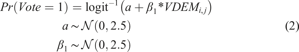

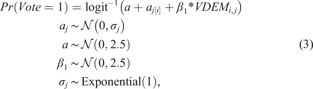
\begin{array}{l} P r (V o t e = 1) = {logit}^{- 1} (a + β_{1} * V D E M_{i, j}) \\ a \sim N (0,2.5) \\ β_{1} \sim N (0,2.5) \end{array}

(2)

where VDem_i,j is the measure of corruption in source country j for which respondent i is dosed, standardized to have mean 0 and standard deviation 1. The last two lines are the prior distributions assigned to a and β₁, with

N (0,2.5)

being the recommended weakly informative Gaussian prior for the intercept and coefficient parameters in logit models (Gelman et al., 2020). Subsequent models expand on (2) by adding the above mentioned controls for individual-level demographic characteristics (i.e., age and sex), election year dummy variables, and source country characteristics (regime type and GDP), all of which also receive the

N (0,2.5)

prior. When estimating the multilevel regressions, (2) is amended to (control variables suppressed)

\begin{array}{l} P r (V o t e = 1) = {logit}^{- 1} (a + a_{j [i]} + β_{1} * V D E M_{i, j}) \\ a_{j} \sim N (0, σ_{j}) \\ a \sim N (0,2.5) \\ β_{1} \sim N (0,2.5) \\ σ_{j} \sim Exponential (1) \end{array},

(3)

where a_j[i] are the country-specific intercepts and the last four lines are the prior distributions.¹⁸

Before presenting the results from estimating (2) and (3), note here that Section 5.1 demonstrates that neither the statistical nor substantive conclusions presented below depend on the use of a Bayesian model.

Results

Table 2 presents the baseline results. Since the models are Bayesian, the estimates refer to the mean of the posterior distribution while the intervals refer to the values that contain 95% of the posterior. Model 1 estimates the bivariate specification in (2). The negative estimate, along with the fact that entirety of the 95% interval is negative indicates that in all likelihood, higher levels of source country corruption corresponds with a lower probability of voting.

Table 2.

The Effect of Corruption on Voter Turnout.

	Model 1	Model 2	Model 3	Model 4	Model 5
Corruption	−0.49 [−0.54; − 0.45]	−0.28 [−0.34; − 0.22]	−0.15 [−0.29; − 0.00]	−0.16 [−0.30; − 0.01]	−0.18 [−0.32; − 0.04]
	−0.49 [−0.54; − 0.45]	−0.28 [−0.34; − 0.22]	−0.15 [−0.29; − 0.00]	−0.16 [−0.30; − 0.01]	−0.18 [−0.32; − 0.04]
Regime Type		0.08 [0.02; 0.14]	−0.01 [−0.09; 0.07]	−0.01 [−0.09; 0.07]	−0.01 [−0.09; 0.07]
		0.08 [0.02; 0.14]	−0.01 [−0.09; 0.07]	−0.01 [−0.09; 0.07]	−0.01 [−0.09; 0.07]
Per Capita GDP		−0.06 [−0.10; − 0.01]	0.02 [−0.08; 0.12]	0.02 [−0.08; 0.12]	0.02 [−0.08; 0.12]
		−0.06 [−0.10; − 0.01]	0.02 [−0.08; 0.12]	0.02 [−0.08; 0.12]	0.02 [−0.08; 0.12]
Female		0.23 [0.14; 0.31]	0.25 [0.16; 0.33]	0.25 [0.17; 0.34]	0.26 [0.17; 0.34]
		0.23 [0.14; 0.31]	0.25 [0.16; 0.33]	0.25 [0.17; 0.34]	0.26 [0.17; 0.34]
Age: 30–39		0.53 [0.41; 0.64]	0.53 [0.41; 0.66]	0.54 [0.41; 0.66]	0.54 [0.41; 0.66]
		0.53 [0.41; 0.64]	0.53 [0.41; 0.66]	0.54 [0.41; 0.66]	0.54 [0.41; 0.66]
Age: 40–49		0.72 [0.57; 0.87]	0.74 [0.58; 0.91]	0.77 [0.59; 0.94]	0.77 [0.59; 0.94]
		0.72 [0.57; 0.87]	0.74 [0.58; 0.91]	0.77 [0.59; 0.94]	0.77 [0.59; 0.94]
Age: 50–59		1.06 [0.87; 1.25]	1.10 [0.88; 1.32]	1.13 [0.91; 1.37]	1.15 [0.93; 1.37]
		1.06 [0.87; 1.25]	1.10 [0.88; 1.32]	1.13 [0.91; 1.37]	1.15 [0.93; 1.37]
Age: 60–69		1.34 [1.14; 1.56]	1.39 [1.14; 1.65]	1.43 [1.17; 1.68]	1.45 [1.19; 1.71]
		1.34 [1.14; 1.56]	1.39 [1.14; 1.65]	1.43 [1.17; 1.68]	1.45 [1.19; 1.71]
Age: 70–79		1.24 [1.06; 1.41]	1.32 [1.09; 1.55]	1.36 [1.11; 1.60]	1.39 [1.16; 1.64]
		1.24 [1.06; 1.41]	1.32 [1.09; 1.55]	1.36 [1.11; 1.60]	1.39 [1.16; 1.64]
Age: 80+		0.68 [0.52; 0.83]	0.76 [0.53; 1.00]	0.80 [0.57; 1.03]	0.84 [0.60; 1.07]
		0.68 [0.52; 0.83]	0.76 [0.53; 1.00]	0.80 [0.57; 1.03]	0.84 [0.60; 1.07]
Year: 2004		0.10 [−0.05; 0.24]	0.11 [−0.04; 0.25]	0.09 [−0.06; 0.24]	0.07 [−0.09; 0.24]
		0.10 [−0.05; 0.24]	0.11 [−0.04; 0.25]	0.09 [−0.06; 0.24]	0.07 [−0.09; 0.24]
Year: 2008		0.40 [0.25; 0.54]	0.42 [0.27; 0.57]	0.41 [0.26; 0.57]	0.39 [0.22; 0.56]
		0.40 [0.25; 0.54]	0.42 [0.27; 0.57]	0.41 [0.26; 0.57]	0.39 [0.22; 0.56]
Year: 2012		0.17 [0.03; 0.29]	0.16 [0.02; 0.30]	0.15 [0.00; 0.29]	0.12 [−0.04; 0.28]
		0.17 [0.03; 0.29]	0.16 [0.02; 0.30]	0.15 [0.00; 0.29]	0.12 [−0.04; 0.28]
Year: 2016		0.25 [0.11; 0.38]	0.26 [0.11; 0.41]	0.26 [0.11; 0.40]	0.23 [0.07; 0.40]
		0.25 [0.11; 0.38]	0.26 [0.11; 0.41]	0.26 [0.11; 0.40]	0.23 [0.07; 0.40]
Intercept	0.60 [0.56; 0.64]	−0.23 [−0.35; − 0.10]	−0.07 [−0.25; 0.10]	−0.10 [−0.30; 0.09]	−0.12 [−0.31; 0.07]
	0.60 [0.56; 0.64]	−0.23 [−0.35; − 0.10]	−0.07 [−0.25; 0.10]	−0.10 [−0.30; 0.09]	−0.12 [−0.31; 0.07]
Num. Obs.	10796	10796	10796	10796	10796
Std Dev: Country			0.41	0.41	0.40
Std Dev: State				0.24
Std Dev: Metro					0.28

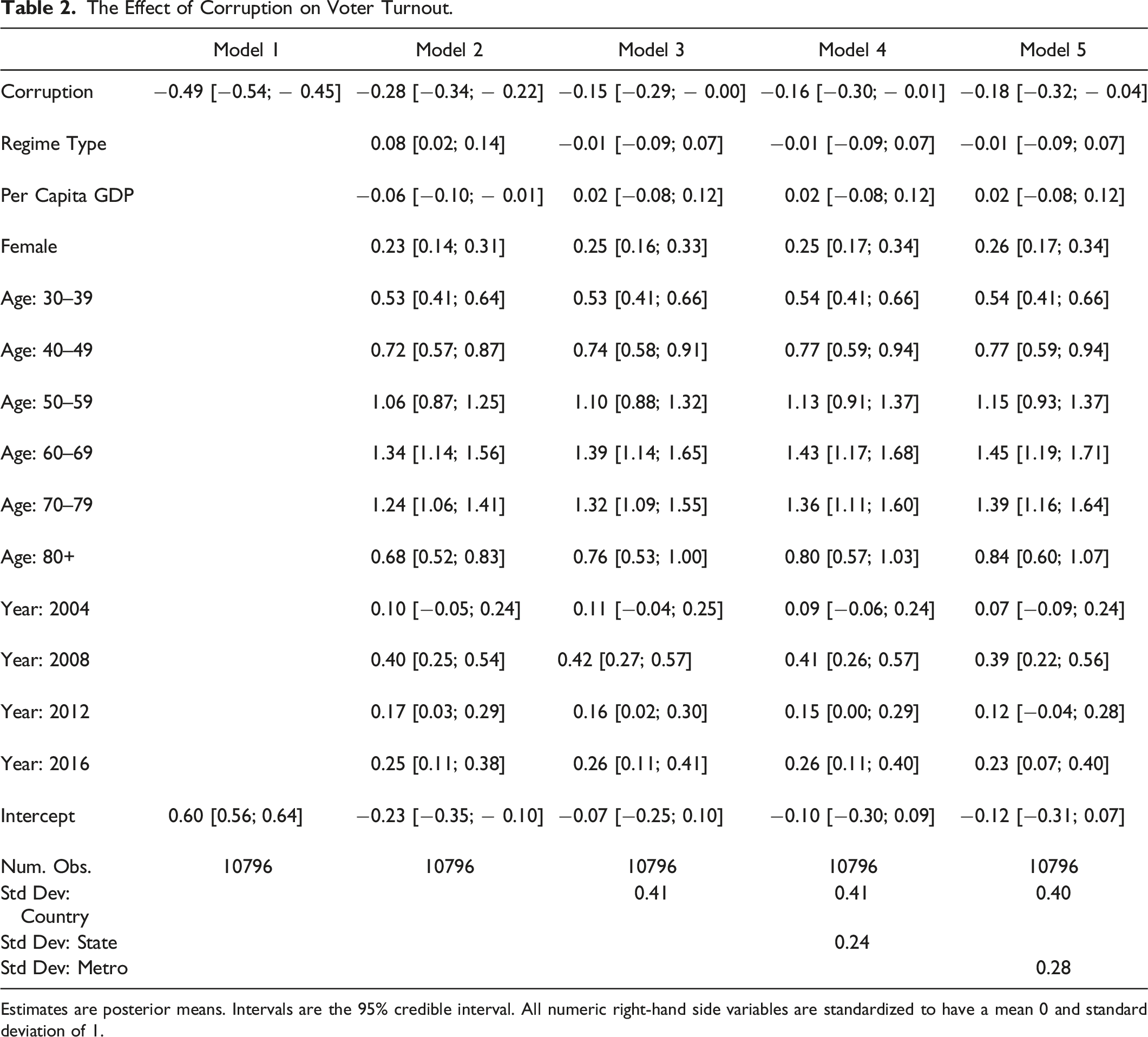
Estimates are posterior means. Intervals are the 95% credible interval. All numeric right-hand side variables are standardized to have a mean 0 and standard deviation of 1.

The remaining models in Table 2 address omitted variable bias in various ways. Model 2 controls for the ancestral country’s regime type, its per capita GDP, and the aforementioned demographic and election year dummy variables. The negative effect of corruption remains, though the effect is smaller in magnitude when compared to Model 1. Model 3 continues by estimating the full multilevel model that allows the intercept to vary by respondent’s ancestral country, to account for any lingering unmeasured country-specific confounding factors. These results continue to show a negative effect of corruption on turnout. A figure can clarify both the statistical and substantive effects. Accordingly, based on the Model 3 results, panel a in Figure 3 plots the posterior distribution of β₁, while also identifying the posterior mean and the intervals containing 66%, 90%, and 95% of the distribution. For reference, the plot also displays 0 on the number line. Notice first that 95% of the posterior distribution is less than zero, suggesting that the true relationship between source country corruption and turnout is very likely a negative one.

Figure 3.

Posterior plots for Model 3 in Table 2. Panel a plots the posterior distribution for β₁, along with the posterior mean and the 66%, 90%, and 95% intervals, based on 4000 draws of the posterior (1000 draws for each of four Markov chains). Panel b plots the predicted probability of voting, throughout the range of V-DEM in the sample, along with the posterior distribution of predictions. Panel c plots the AME of a one standard deviation increase in source country corruption.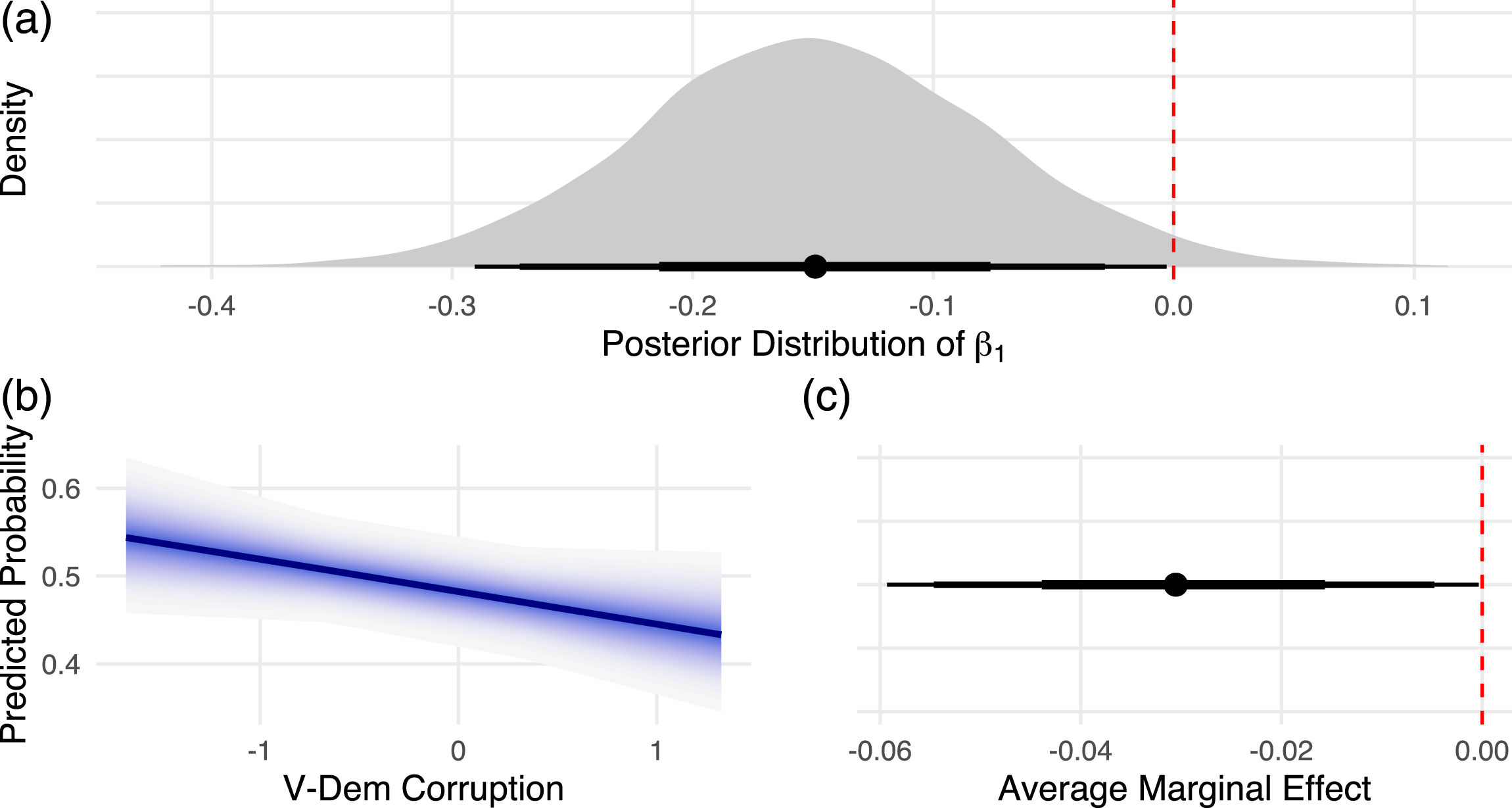

The substantive impact of corruption implied by Model 3 is appreciable. Panel b of Figure 3 demonstrates by plotting the predicted probability of voting across the range of source country corruption in the sample, while holding the control variables at their mean values or reference category. The ribbon around the prediction line contains the distribution of posterior predictions, with the darker portions thereof corresponding to the more densely populated areas of the posterior. Moving from the minimum value of source country corruption in this sample (−1.7 units below the mean, corresponding to a value equal to 0.003 on the original 0–1 scale) to the maximum value (1.5 units above the mean; 0.96 on the 0–1 scale) reduces the probability of voting by about 10 points, from a probability of 0.55 to 0.45. Finally, Panel c follows the advice in Hanmer and Kalkan (2013), and calculates the average marginal effect of corruption on turnout across the observed values of the control variables in the sample. Doing so reveals that a one standard deviation increase in source country corruption reduces the probability of voting, on average, by 0.03, with a 95% interval extending between [−0.06; − 0.0003].¹⁹

Lastly, Models 4 and 5 in Table 2 address the facts that immigrants do not settle across the U.S. in random patterns, but rather often cluster in particular states, metropolitan areas, and neighborhoods (Bartel, 1989). This matters because a locality’s level of political engagement is reproduced in its residents (Cho et al., 2006; Gimpel et al., 2003; Huckfeldt & Sprague, 1987). As Cho et al. (2006) put it, “whatever the roots of a place’s participatory behavior, living in some locations facilitates learning the political ropes, while living in other areas does not” (p. 156). Similarly, states and localities differ in the hurdles they erect for their residents to vote. To assess whether these contextual factors affect the results, Model 4 estimates a multilevel model that allows the intercept to vary both by country of ancestry and by the respondent’s state of residence, while Model 5 allows the intercept to vary by both ancestral country and the respondent’s metropolitan area. Neither specification materially changes the conclusions.²⁰

Before assessing the sensitivity of these results, we briefly discuss the models’ control variables. Though caution is appropriate when assigning causality to control variables (Keele et al., 2020), several associations are worth mentioning. For instance, the Table 2 results show the familiar pattern with respect to age, in which older respondents have a higher probability of voting that younger ones do, with that relationship declining in strength among respondents aged 80 years or more. And in this sample, we find that women have a higher probability of voting than men. Interestingly, there is no robust evidence that turnout is associated with either the ancestral country’s regime type or its level of economic development. Though both of those variables are associated with turnout in Model 2 (positive for regime type; negative for per capita GDP), the associations disappear in the subsequent multilevel models.

Sensitivity Checks

The Table 2 results are reassuringly robust. First, a common critique of Bayesian approaches is that the explicit specification of priors may allow researchers’ expectations to affect the results. To ensure this is not the case, in Tables 3, I re-estimate all of the models with maximum likelihood techniques instead of Bayesian ones. The results reach the same substantive conclusions as in Table 2.

Table 3.

Maximum Likelihood Results.

	Model 1	Model 2	Model 3	Model 4	Model 5
Corruption	−0.49*** (0.02)	−0.28*** (0.03)	−0.15** (0.07)	−0.15** (0.07)	−0.17** (0.07)
	−0.49*** (0.02)	−0.28*** (0.03)	−0.15** (0.07)	−0.15** (0.07)	−0.17** (0.07)
Regime Type		0.08*** (0.03)	−0.01 (0.04)	−0.01 (0.04)	−0.01 (0.04)
		0.08*** (0.03)	−0.01 (0.04)	−0.01 (0.04)	−0.01 (0.04)
Per Capita GDP		−0.06** (0.02)	0.03 (0.05)	0.02 (0.05)	0.03 (0.05)
		−0.06** (0.02)	0.03 (0.05)	0.02 (0.05)	0.03 (0.05)
Female		0.23*** (0.04)	0.25*** (0.04)	0.25*** (0.04)	0.26*** (0.04)
		0.23*** (0.04)	0.25*** (0.04)	0.25*** (0.04)	0.26*** (0.04)
Age: 30–39		0.53*** (0.06)	0.53*** (0.06)	0.54*** (0.06)	0.54*** (0.06)
		0.53*** (0.06)	0.53*** (0.06)	0.54*** (0.06)	0.54*** (0.06)
Age: 40–49		0.72*** (0.08)	0.75*** (0.09)	0.77*** (0.09)	0.78*** (0.09)
		0.72*** (0.08)	0.75*** (0.09)	0.77*** (0.09)	0.78*** (0.09)
Age: 50–59		1.06*** (0.10)	1.10*** (0.11)	1.14*** (0.12)	1.17*** (0.12)
		1.06*** (0.10)	1.10*** (0.11)	1.14*** (0.12)	1.17*** (0.12)
Age: 60–69		1.34*** (0.11)	1.40*** (0.13)	1.44*** (0.13)	1.46*** (0.13)
		1.34*** (0.11)	1.40*** (0.13)	1.44*** (0.13)	1.46*** (0.13)
Age: 70–79		1.24*** (0.09)	1.33*** (0.12)	1.37*** (0.12)	1.41*** (0.12)
		1.24*** (0.09)	1.33*** (0.12)	1.37*** (0.12)	1.41*** (0.12)
Age: 80+		0.68*** (0.08)	0.77*** (0.12)	0.81*** (0.12)	0.86*** (0.12)
		0.68*** (0.08)	0.77*** (0.12)	0.81*** (0.12)	0.86*** (0.12)
Year: 2004		0.10 (0.07)	0.11 (0.07)	0.09 (0.08)	0.08 (0.08)
		0.10 (0.07)	0.11 (0.07)	0.09 (0.08)	0.08 (0.08)
Year: 2008		0.40*** (0.07)	0.42*** (0.08)	0.41*** (0.08)	0.39*** (0.09)
		0.40*** (0.07)	0.42*** (0.08)	0.41*** (0.08)	0.39*** (0.09)
Year: 2012		0.17** (0.07)	0.16** (0.07)	0.14** (0.07)	0.12 (0.08)
		0.17** (0.07)	0.16** (0.07)	0.14** (0.07)	0.12 (0.08)
Year: 2016		0.25*** (0.07)	0.26*** (0.07)	0.25*** (0.07)	0.23*** (0.08)
		0.25*** (0.07)	0.26*** (0.07)	0.25*** (0.07)	0.23*** (0.08)
Num. Obs.	10796	10796	10796	10796	10796
Std Dev: Country			0.37	0.39	0.37
Std Dev: State				0.22
Std Dev: Metro					0.26

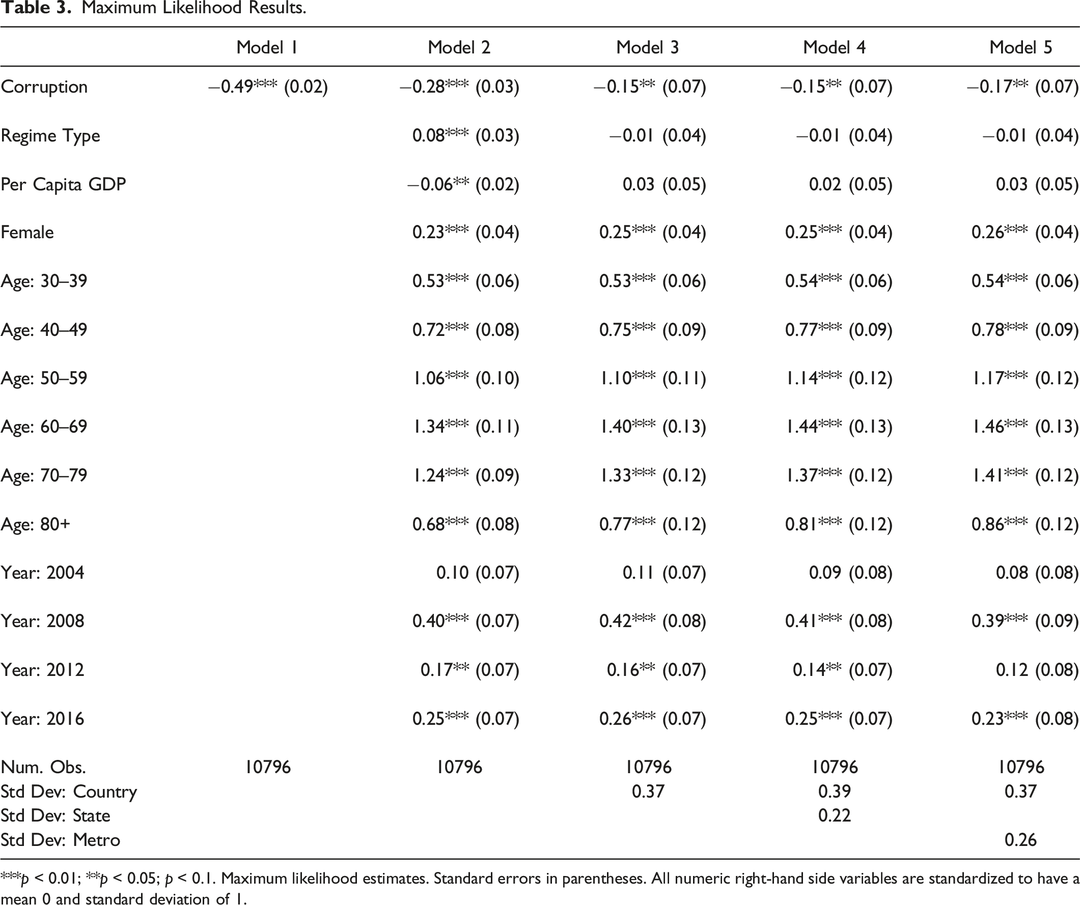
***p < 0.01; **p < 0.05; p < 0.1. Maximum likelihood estimates. Standard errors in parentheses. All numeric right-hand side variables are standardized to have a mean 0 and standard deviation of 1.

A more serious threat to inference regards the role education ought to play in the model. Per Figure 1, I have argued that corruption may affect turnout by lowering SES in general and education outcomes in particular. However, it is also possible that education affects equilibrium levels of corruption. Indeed, Uslaner and Rothstein (2016) show schooling rates in 1870 influence contemporary levels of corruption, because education raises public awareness, reduces the demand for clientelism, increases social trust, and spurs economic development.²¹ Notice that accepting the Uslaner and Rothstein (2016) result while maintaining the presumption that education is internationally mobile and reproduced inter-generationally implies that the estimates of corruption’s effects in Table 2 may be confounded. Rather than corruption affecting turnout, it could be that historical schooling rates determine both contemporary levels of corruption and the turnout choices of today’s second generation Americans.

To assess whether this is the case, I re-estimate the models in Table 2 while controlling for the average number of years of schooling in source country i in 1870, per Uslaner and Rothstein (2016).²² The numerical summary of the results can be found in Table A1, but pay attention to Figure 4, which plots the posterior distribution of the corruption parameter for each of the five models. Adding historical rates of schooling to the model does not alter the substantive conclusions much. The one slight change is that in Models 3 and 4, the 95% interval includes positive effects, but even in those cases, 93% of the posterior is negative, suggesting that there remains a very high likelihood that the true impact of corruption is a negative one.

Figure 4.

The effect of corruption on turnout when controlling for average schooling rates in source country i in 1870. Figure shows the posterior distribution for β₁ for five models, along with the posterior mean and the 66%, 90%. and 95% intervals. These results are based on 4000 draws of the posterior (1000 draws for each of four Markov chains). A numerical summary of the results is displayed in Table A1.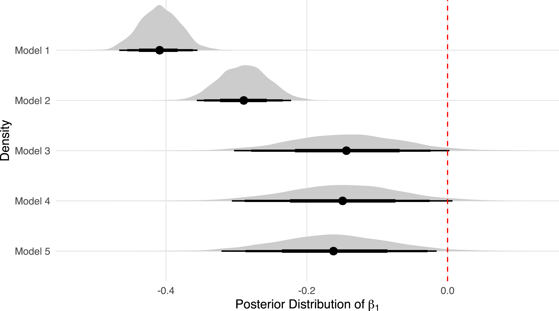

Lastly, as discussed above, it is not obvious whether we should match respondents according to their maternal or paternal ancestry. The models presented thus far sample only those respondents for whom the parents are both immigrants to the United States and from the same country, but Tables A2 and A3 in the Appendix match the respondents with their maternal (Table A2) and paternal (Table A3) ancestral country, respectively, regardless of the nationality of the other parent. These results continue to show a negative and statistically reliable effect of corruption on turnout. The one difference is that in Model 4 of Table A3, there is slightly more uncertainty regarding corruption’s effect since less than 95% of the posterior is negative, though more than 90% of it is.

Considering the SES Mechanism

The accumulated results thus indicate a statistically reliable and substantively sizable negative effect of corruption on turnout. Importantly, the result does not suffer from reverse causality, nor is it confounded by a country’s level of economic development, its degree of democracy, some unmeasured factor that residents of the same ancestral country share, or some unmeasured confound pertaining to state or locality in which the CPS respondent currently lives. Though these results are important in their own right, this paper also hopes to contribute to our understanding regarding why corruption might exert this effect. As discussed above, existing studies emphasize corruption’s material consequences for citizens and its implications for their feelings of civic duty. Without dismissing these possibilities, I have suggested that the causal effect might also be transmitted by SES, since education and income are reliable predictors of whether one votes and corruption affects how much education one acquires and how much income one makes (Chua, 1999, 2000a; 2000b; Duerrenberger & Warning, 2018; Ferraz et al., 2012; Suryadarma, 2012).

To test this novel SES pathway, I estimate several additional regressions. Model 1 in Table 4 begins by predicting the level of schooling of second generation Americans with the level of corruption in the ancestral country. The schooling survey instrument is a categorical variable in the CPS and I recode it to have four levels: no high school degree, a high school degree, some college, and college graduate. The regression is therefore an ordered logit model that controls for the respondent’s sex, age, family income, year dummy variables, along with the source country’s regime type, per capita GDP, and historical (i.e., 1870) schooling levels. Estimation proceeds in a Bayesian multilevel framework with respondents clustered according to their country of ancestry and with weakly informative priors assigned to all model parameters. To ensure the schooling results are not influenced by the presence of younger respondents who have not had the chance to attend or graduate college, the sample includes only individuals aged at least 22 years.

Table 4.

The Effect of Corruption on Schooling Attainment and Family Income.

	Schooling	Family income	Turnout
	Model 1^a	Model 2^b	Model 3
Corruption	−0.20 [−0.40; − 0.03]	−0.19 [−0.34; − 0.03]
	−0.20 [−0.40; − 0.03]	−0.19 [−0.34; − 0.03]
Regime Type	−0.06 [−0.14; 0.02]	−0.09 [−0.17; − 0.00]
	−0.06 [−0.14; 0.02]	−0.09 [−0.17; − 0.00]
Per Capita GDP	−0.06 [−0.20; 0.07]	−0.11 [−0.21; − 0.01]
	−0.06 [−0.20; 0.07]	−0.11 [−0.21; − 0.01]
Female	0.15 [0.07; 0.23]	−0.23 [−0.31; − 0.15]	0.23 [0.15; 0.32]
	0.15 [0.07; 0.23]	−0.23 [−0.31; − 0.15]	0.23 [0.15; 0.32]
Age: 30–39	0.06 [−0.07; 0.20]	0.48 [0.37; 0.59]	0.31 [0.18; 0.42]
	0.06 [−0.07; 0.20]	0.48 [0.37; 0.59]	0.31 [0.18; 0.42]
Age: 40–49	−0.24 [−0.42; − 0.04]	0.66 [0.51; 0.81]	0.59 [0.42; 0.73]
	−0.24 [−0.42; − 0.04]	0.66 [0.51; 0.81]	0.59 [0.42; 0.73]
Age: 50–59	−0.33 [−0.58; − 0.09]	0.40 [0.20; 0.59]	1.04 [0.84; 1.24]
	−0.33 [−0.58; − 0.09]	0.40 [0.20; 0.59]	1.04 [0.84; 1.24]
Age: 60–69	−0.71 [−0.98; − 0.44]	0.11 [−0.15; 0.36]	1.57 [1.35; 1.81]
	−0.71 [−0.98; − 0.44]	0.11 [−0.15; 0.36]	1.57 [1.35; 1.81]
Age: 70–79	−1.07 [−1.34; − 0.80]		1.82 [1.61; 2.01]
	−1.07 [−1.34; − 0.80]		1.82 [1.61; 2.01]
Age: 80+	−1.67 [−1.99; − 1.39]		1.49 [1.28; 1.67]
	−1.67 [−1.99; − 1.39]		1.49 [1.28; 1.67]
Year: 2004	0.09 [−0.04; 0.23]	0.39 [0.24; 0.54]	0.01 [−0.13; 0.17]
	0.09 [−0.04; 0.23]	0.39 [0.24; 0.54]	0.01 [−0.13; 0.17]
Year: 2008	0.24 [0.10; 0.38]	0.74 [0.59; 0.89]	0.22 [0.07; 0.37]
	0.24 [0.10; 0.38]	0.74 [0.59; 0.89]	0.22 [0.07; 0.37]
Year: 2012	0.37 [0.23; 0.51]	0.61 [0.47; 0.76]	−0.07 [−0.20; 0.08]
	0.37 [0.23; 0.51]	0.61 [0.47; 0.76]	−0.07 [−0.20; 0.08]
Year: 2016	0.41 [0.26; 0.57]	0.94 [0.80; 1.09]	−0.03 [−0.18; 0.11]
	0.41 [0.26; 0.57]	0.94 [0.80; 1.09]	−0.03 [−0.18; 0.11]
Family Income: Lower Middle	0.62 [0.51; 0.73]		0.34 [0.22; 0.46]
	0.62 [0.51; 0.73]		0.34 [0.22; 0.46]
Family Income: Middle	1.16 [1.04; 1.30]		0.53 [0.39; 0.68]
	1.16 [1.04; 1.30]		0.53 [0.39; 0.68]
Family Income: Upper Middle	1.66 [1.51; 1.81]		0.45 [0.28; 0.61]
	1.66 [1.51; 1.81]		0.45 [0.28; 0.61]
Family Income: Upper	1.98 [1.84; 2.14]		0.72 [0.56; 0.88]
	1.98 [1.84; 2.14]		0.72 [0.56; 0.88]
Average Years of Schooling (1870)	−0.02 [−0.22; 0.16]
	−0.02 [−0.22; 0.16]
Schooling: Graduate High School		0.62 [0.48; 0.77]	0.58 [0.45; 0.72]
		0.62 [0.48; 0.77]	0.58 [0.45; 0.72]
Schooling: Some College		1.02 [0.87; 1.17]	1.16 [1.01; 1.31]
		1.02 [0.87; 1.17]	1.16 [1.01; 1.31]
Schooling: Graduate College		1.78 [1.64; 1.94]	1.67 [1.52; 1.82]
		1.78 [1.64; 1.94]	1.67 [1.52; 1.82]
Intercept			−1.40 [−1.63; − 1.19]
			−1.40 [−1.63; − 1.19]
Std Dev: Country	0.51	0.46	0.42
Num. obs.	8882	7832	10796

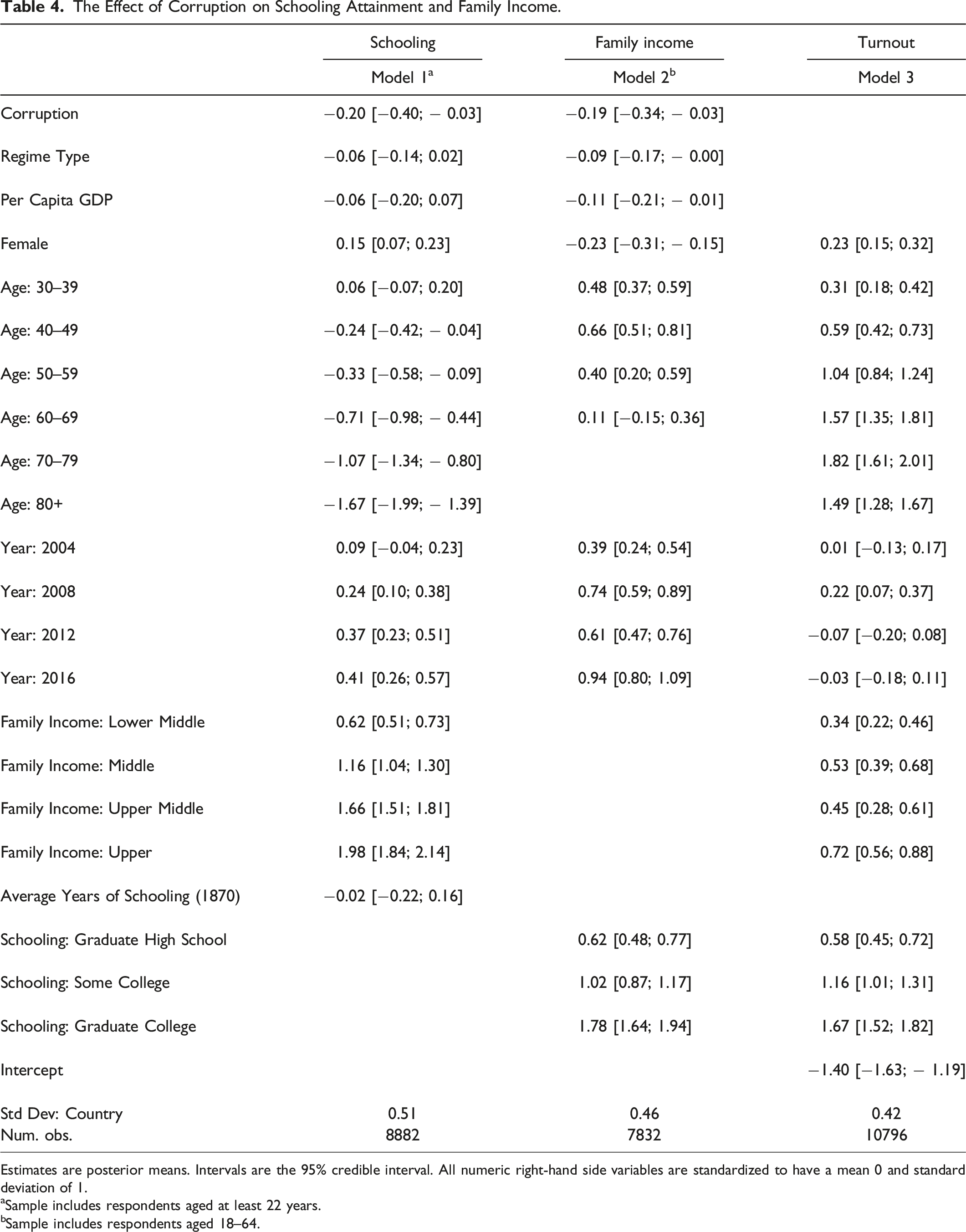
Estimates are posterior means. Intervals are the 95% credible interval. All numeric right-hand side variables are standardized to have a mean 0 and standard deviation of 1.

^aSample includes respondents aged at least 22 years.

^bSample includes respondents aged 18–64.

The model’s estimate indicates that, indeed, source country corruption correlates negatively with schooling attainment of second generation Americans. Figure 5 plots the predicted probabilities implied by the coefficient estimates. Holding the control variables at their mean values or reference categories, an increase in corruption from the sample minimum to its maximum, increases the probabilities the respondent does not finish high school (from 0.1 to 0.17) and the probability that a high school diploma is one’s terminal degree (0.33–0.42), while decreasing the probability of graduating college (0.33–0.2).

Figure 5.

Lines plot the predicted probabilities of obtaining various levels of schooling, throughout the range of V-DEM in the sample and the 95% of intervals around the predictions.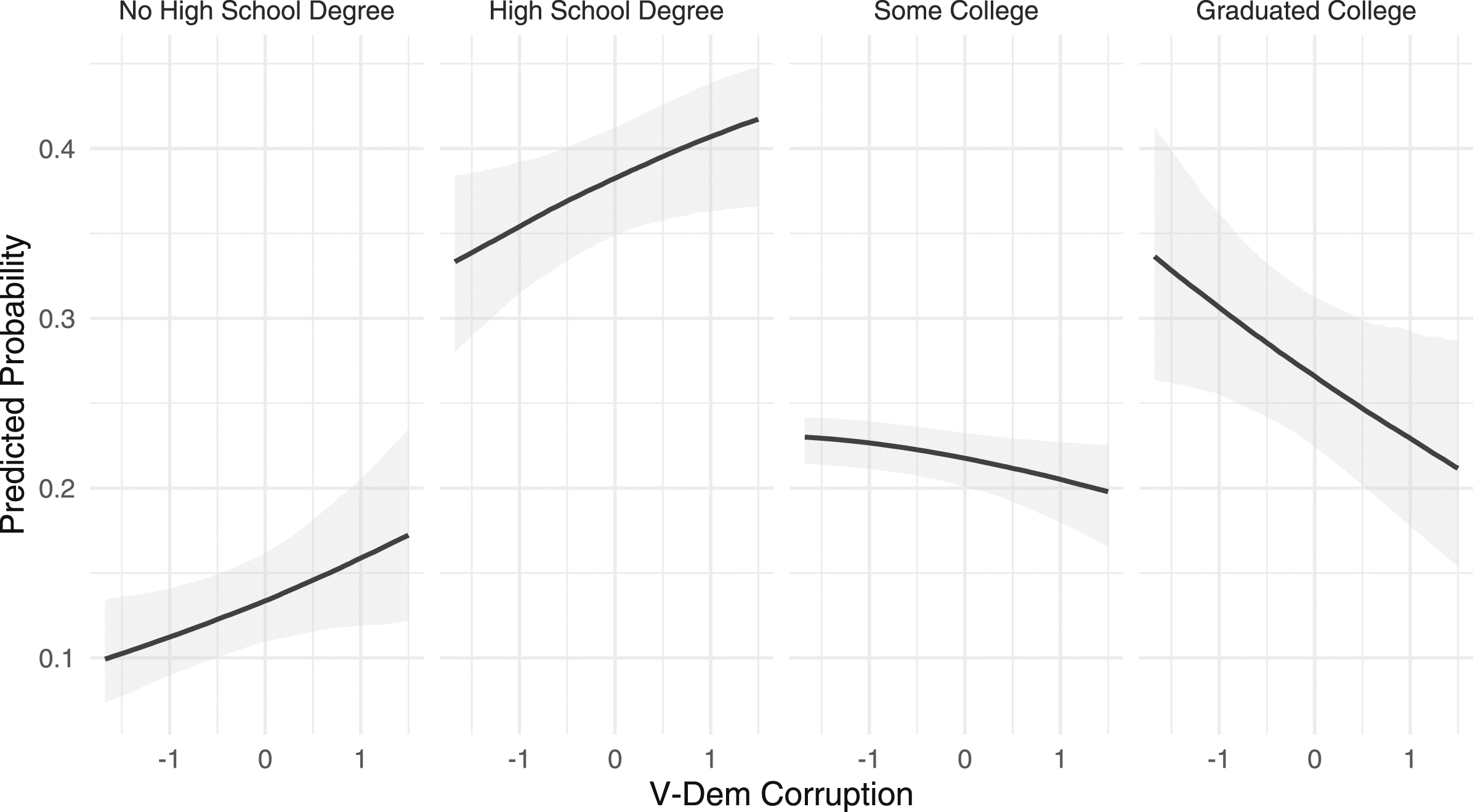

Model 2 operationalizes SES in terms of one’s family income, a categorical variable recoded to have five levels: low income, lower-middle, middle, upper-middle, and upper income.²³ This regression is also a multilevel ordered logit model—estimated in a Bayesian multilevel framework—that controls for respondent demographics, year dummy variables, and the source country characteristics. To ensure that the results are not overly determined by respondents who have retired, the sample includes only respondents aged 64 years or less.²⁴ Consistent with expectations, Model 2 shows a negative effect of corruption on family income.

For sake of completeness, Model 3 attempts to replicate the common result that schooling and income correlate positively with the decision to vote and finds it easy to do so. Every income category increases the probability the respondent votes compared to the reference category of low income. Likewise, every increase in schooling increases the probability of voting compared to a respondent who did not finish high school. Combining all the results in Tables 4, it follows that corruption appears to affect turnout not just through its effects on civic duty and the material benefits one can expect to accrue through voting, but also by affecting whether individuals possess sufficient stocks of valuable participatory resources.

Conclusion

This paper contributes to the ongoing and robust debate regarding the consequences of corruption for citizen engagement and voter turnout. As has been discussed, any number of factors may explain the lack of consensus with respect to corruption’s effects, but one empirical dilemma lingering over all observational studies in this tradition is reverse causality. Democratic theory tells us that citizen engagement is necessary for good governance, the implication being that estimates of corruption’s effects on turnout may be biased, unless appropriate adjustments are made. Making those adjustments can be difficult though since finding good instruments is notoriously challenging and bad ones just make the problem worse (Bound et al., 1995).

To tackle the endogeneity problem, this paper advances two related claims. First, the effects of corruption need not be bound to the country where the corruption occurred. Rather, because education, accumulated wealth, and political dispositions—some of the most important predictors of turnout choices—are endogenous to corruption and internationally mobile, a country’s level of corruption can affect the participation choices of its émigrés. Second, because those attributes are passed on inter-generationally within the family, the consequences of corruption may also be inter-generational. These facts suggest a research design that is not subject to reverse causality, namely, a model that regresses the turnout choices of second generation Americans on the level of corruption in their country of ancestry. Estimating such a model shows a statistically reliable and substantively appreciable negative effect of corruption on turnout. Though this is not the first paper to report a negative effect, it is one of the few observational studies that explicitly addresses the reverse causality problem.²⁵ Thus, it bolsters some existing studies (e.g., Caillier, 2010; McCann & Domínguez, 1998; Sundström & Stockemer, 2015) by showing the robustness of the negative effect.

There is also a theoretical contribution in this paper. Given the robust correlations between, on one hand, SES and turnout and, on the other hand, corruption and SES, it is somewhat surprising that existing scholarship has not linked corruption to turnout along an SES pathway. I have done so here and presented evidence consistent with that pathway. Thus, along with the other ways corruption affects turnout (e.g., civic duty and the material benefits to voting), it appears that corruption may also transmit its effect through SES. Future scholarship ought to probe this mechanism further.

There are several ways that future research could improve upon and extend this study. Most obviously, this study is limited to turnout in US elections. There is value in applying the method used here to other countries to assess whether it continues to hold or whether there is something peculiar about the United States, its immigrants, and its second generation citizens. One could even apply the model to internal migration—assessing, for instance, how early socialization experiences in, say, notoriously corrupt Louisiana affects the participation choices of those who have since moved out of that state and into another.²⁶

Secondly, though this paper uses the behavioral patterns of second generation Americans to identify the causal effect of corruption, it leaves unanswered a pertinent question, namely, how long do the effects of source country corruption last? Should we expect second generation Americans with ancestry in corrupt countries to have a lower probability of voting permanently? Or, will socialization processes cause them to regress to the mean? Existing evidence tends to favor the latter possibility. For instance Wals and Rudolph (2018) show how acculturation reduces the salience of premigratory experiences for Mexican immigrants to the United States. Note though that Wals and Rudolph (2018) study the immigrants themselves; whether similar processes operate on their American-born children who are the subject of the present study remains an open question.²⁷ These are important questions and answering them will improve understanding of the political behavior of US immigrants and their children. Nevertheless, addressing them is beyond the scope of the present study.

Third, though this study endeavors to identify a causal effect of corruption, it abstracts away from the question of whether corruption perceptions have different effects on citizen engagement than experiences with corruption or convictions of corrupt officials. This is an ongoing area of research though and these distinctions are also likely to contribute to the lack of consensus in existing research.²⁸ However, the data employed in this study does not allow us to distinguish between these possibilities.

Lastly, this paper has focused on the supply-side of the vote function, ignoring politicians’ demand for votes and their mobilization strategies. It is possible that supply and demand offset each other. This would occur if corruption reduces SES and civic duty but increases turnout buying, à la Escaleras et al. (2012); Lacombe et al. (2016) and Karahan et al. (2006), or if corruption increases mobilization efforts by opposition parties who subsequently find their efforts challenged by an alienated and resource constrained citizenry (Davis et al., 2004). The nature of the design used here rules out such possibilities because the mobilization strategies of US parties is unrelated to corruption levels in the various source countries. In that regard, this research design emphasizes the supply-side of voter turnout. Further consideration of the demand side of the problem and the way supply and demand interact would convey useful information regarding the net effect of corruption.

Footnotes

Declaration of Conflicting Interests

The author(s) declared no potential conflicts of interest with respect to the research, authorship, and/or publication of this article.

Funding

The author(s) received no financial support for the research, authorship, and/or publication of this article.

ORCID iD

Joel W. Simmons

Notes

Appendix

Author Biography

Joel W. Simmons is an Associate Professor in the Walsh School of Foreign Service and the Department of Government at Georgetown University. His research focuses on the political economy of development, with emphases in economic growth, social policy, global economic integration, corruption, the political economy of gender, and the effect of political parties and party systems on development outcomes.

References

Achen

C. H.

(2002). Parental socialization and rational party identification. Political Behavior, 24(2), 151–170. https://doi.org/10.1023/A:1021278208671

Adserà

Boix

Payne

(2003). Are you being served? Political accountability and quality of government. The Journal of Law, Economics, and Organization 19(2), 445–490. https://doi.org/10.1093/jleo/ewg017

Almond

G. A.

Verba

(1963). The civic culture: Political attitudes and democracy in five nations. Little, Brown, and Company.

Anderson

C. J.

Tverdova

Y. V.

(2003). Corruption, political allegiances, and attitudes toward government in contemporary democracies. American Journal of Political Science, 47(1), 91–109. https://doi.org/10.1111/1540-5907.00007

Antecol

(2000). An examination of cross-country differences in the gender gap in labor force participation rates. Labour Economics, 7(4), 409–426. https://doi.org/10.1016/s0927-5371(00)00007-5

Barry

(1970). Sociologists, economists, and democracy. Collier-Macmillan.

Bartel

A. P.

(1989). Where do the new U.S. Immigrants live? Journal of Labor Economics 7(4), 371–391. https://doi.org/10.1086/298213. http://www.jstor.org/stable/2535134

Baum

M. A.

Lake

D. A.

(2003). The political economy of growth: Democracy and human capital. American Journal of Political Science 47(2), 333–347. https://doi.org/10.1111/1540-5907.00023. http://www.jstor.org/stable/3186142

Bazurli

Portos

(2019). Crook!: The impact of perceived corruption on non-electoral forms of political behaviour. International Political Science Review, 42(2), 245–260. https://doi.org/10.1177/0192512119881710

10.

Blau

F. D.

Kahn

L. M.

Papps

K. L.

(2011). Gender, source country characteristics, and labor market assimilation among immigrants. The Review of Economics and Statistics, 93(1), 43–58. https://doi.org/10.1162/rest_a_00064

11.

Bolt

van Zanden

J. L.

(2020). Maddison style estimates of the evolution of the world economy. A new 2020 update. Maddison Project Database. version 2020.

12.

Borjas

G. J.

(1993). The intergenerational mobility of immigrants. Journal of Labor Economics 11(1, Part 1), 113–135. https://doi.org/10.1086/298319. http://www.jstor.org/stable/2535186

13.

Bound

Jaeger

D. A.

Baker

R. M.

(1995). Problems with instrumental variables estimation when the correlation between the instruments and the endogenous explanatory variable is weak. Journal of the American Statistical Association, 90(430), 443–450. https://doi.org/10.1080/01621459.1995.10476536

14.

Bowler

Karp

J. A.

(2004). Politicians, scandals, and trust in government. Political Behavior 26(3), 271–287. https://doi.org/10.1023/b:pobe.0000043456.87303.3a. https://www.jstor.org/stable/4151353

15.

Brady

H. E.

Verba

Schlozman

K. L.

(1995). Beyond SES: A resource model of political participation. The American Political Science Review 89(2), 271–294. https://doi.org/10.2307/2082425. https://www.jstor.org/stable/2082425

16.

Bueker

C. S.

(2005). Political incorporation among immigrants from ten areas of origin: The persistence of source country effects. The International Migration Review 39(1), 103–140. https://doi.org/10.1111/j.1747-7379.2005.tb00257.x. https://www.jstor.org/stable/27645478

17.

Bürkner

P.-C.

(2017). brms: An R package for Bayesian multilevel models using stan. Journal of Statistical Software, 80(1), 1–28. https://doi.org/10.18637/jss.v080.i01

18.

Caillier

(2010). Citizen trust, political corruption, and voting behavior: Connecting the dots. Politics & Policy, 38(5), 1015–1035. https://doi.org/10.1111/j.1747-1346.2010.00267.x

19.

Caselli

Morelli

(2004). Bad politicians. Journal of Public Economics, 88(3–4), 759–782. https://doi.org/10.1016/s0047-2727(03)00023-9

20.

Cho

W. K. T.

Gimpel

J. G.

Dyck

J. J.

(2006). Residential concentration, political socialization, and voter turnout. The Journal of Politics, 68(1), 156–167. https://doi.org/10.1111/j.1468-2508.2006.00377.x

21.

Chong

AnaDe La

L.O.

Dean

Leonard

(2015). Does corruption information inspire the fight or quash the hope? A field experiment in Mexico on voter turnout, choice and party identification. The Journal of Politics, 77(1), 55–71. https://doi.org/10.1086/678766

22.

Cho

W. K. T.

(1999). Naturalization, socialization, participation: Immigrants and (Non-)Voting. The Journal of Politics, 61(4), 1140–1155. http://www.jstor.org/stable/2647557

23.

Chua

Y. T.

(1999). Robbed: An investigation of corruption in Philippine education. Philippine Center for Investigative Journalism.

24.

Chua

Y. T.

(2000a). The plunder of textbook funds. In Colonel

S. S.

(Ed.), Betrayals of the public trust: Investigative reports of corruption. Philippine Center for Investigative Journalism.

25.

Chua

Y. T.

(2000b). Stealing from public schools. In Colonel

S. S.

(Ed.), Betrayals of the public trust: Investigative reports of corruption. Philippine Center for Investigative Journalism.

26.

Coppedge

Gerring

Knutsen

C. H.

Lindberg

S. I.

Jan

Alizada

Altman

Bernhard

Cornell

Steven Fish

Gastaldi

Gjerløw

Glynn

Allen

Garry Hindle Ilchenko

Krusell

uhrmann

A. L.

Maerz

S. F.

Marquardt

K. L.

Ziblatt

(2021). V-dem [Country-Year/Country-Date] dataset v9. Varieties of Democracy (V-Dem) Project. https://www.v-dem.net/en/data/data-version-11/

27.

Costas-Pérez

(2014). Political corruption and voter turnout: Mobilization or disaffection? IEB Working Paper N. 2014/27. http://dx.doi.org/10.2139/ssrn.2471065

28.

Dahlberg

Solevid

(2016). Does corruption suppress voter turnout? Journal of Elections, Public Opinion and Parties, 26(4), 489–510. https://doi.org/10.1080/17457289.2016.1223677

29.

Dalton

R. J.

(1988). Citizen politics: Public opinion and political parties in advanced industrial democracies (3rd ed.). Chatham House Publishers.

30.

Davis

C. L.

Camp

R. A.

Coleman

K. M.

(2004). The influence of party systems on Citizens’Perceptions of corruption and electoral response in Latin America. Comparative Political Studies, 37(6), 677–703. https://doi.org/10.1177/0010414004265879

31.

Duerrenberger

Warning

(2018). “Corruption and education in developing countries: The role of public vs. private funding of higher education.” International Journal of Educational Development 62, 217–225. https://doi.org/10.1016/j.ijedudev.2018.05.002. https://www.sciencedirect.com/science/article/pii/S0738059317305813

32.

Escaleras

Calcagno

P. T.

Shughart

W. F.

(2012). Corruption and voter participation: Evidence from the US states. Public Finance Review, 40(6), 789–815. https://doi.org/10.1177/1091142112446846

33.

Feitosa

(2020). Theoretically, yes, but also empirically? How the corruption-turnout link is marginally explained by civic duty to vote. Electoral Studies 66, 102162. https://doi.org/10.1016/j.electstud.2020.102162. https://www.sciencedirect.com/science/article/pii/S0261379420300469

34.

Ferejohn

(1986). Incumbent performance and electoral control. Public Choice 50(1–3), 5–25. https://doi.org/10.1007/bf00124924. http://www.jstor.org/stable/30024650

35.

Fernández

Fogli

(2009). Culture: An empirical investigation of Beliefs, work, and fertility. American Economic Journal: Macroeconomics, 1(1), 146–177. https://doi.org/10.1257/mac.1.1.146

36.

Ferraz

Finan

Moreira

D. B.

(2012). Corrupting learning: Evidence from missing federal education funds in Brazil. Journal of Public Economics 96(9–10), 712–726. https://doi.org/10.1016/j.jpubeco.2012.05.012. https://www.sciencedirect.com/science/article/pii/S0047272712000618

37.

Finseraas

Kotsadam

Polavieja

(2020). Ancestry culture, assimilation, and voter turnout in two generations. Political Behavior, 44(1), 201–226. https://doi.org/10.1007/s11109-020-09617-2

38.

Fiorina

M. P.

(1981). Retrospective voting in American elections. Yale Univeristy Press.

39.

Fisman

Miguel

(2007). Corruption, norms, and legal enforcement: Evidence from diplomatic parking tickets. Journal of Political Economy 115(6), 1020–1048. https://doi.org/10.1086/527495. http://www.jstor.org/stable/10.1086/527495

40.

Flood

King

Rodgers

Ruggles

Robert Warren

(2020). Integrated public use microdata series, current population survey: Version 8.0 [dataset]. https://doi.org/10.18128/D030.V8.0

41.

Gelman

Hill

(2007). Data Analysis Using Regression and Multilevel/Hierarchical Models. Analytical methods for social research Cambridge. Cambridge University Press.

42.

Gelman

Hill

Aki

(2020). Regression and other stories. Analytical methods for social research. Cambridge University Press.

43.

Gimpel

J. G.

Celeste Lay

Schuknecht

J. E.

(2003). Cultivating democracy. Brookings Institution Press.

44.

Giommoni

(2021). Exposure to corruption and political participation: Evidence from Italian municipalities. European Journal of Political Economy 68, 102000. https://doi.org/10.1016/j.ejpoleco.2021.102000. https://www.sciencedirect.com/science/article/pii/S017626802100001X

45.

Giuliano

(2007). Living arrangements in western europe: Does cultural origin matter? Journal of the European Economic Association, 5(5), 927–952. https://doi.org/10.1162/JEEA.2007.5.5.927

46.

Glaeser

E. L.

La Porta

Lopez-de-Silanes

Shleifer

(2004). Do institutions cause growth? Journal of Economic Growth, 9(3), 271–303. https://doi.org/10.1023/b:joeg.0000038933.16398.ed

47.

Glaeser

E. L.

Saks

R. E.

(2006). Corruption in America. Journal of Public Economics, 90(6–7), 1053–1072. https://doi.org/10.1016/j.jpubeco.2005.08.007

48.

Gründler

Potrafke

(2019). Corruption and economic growth: New empirical evidence. European Journal of Political Economy 60, 101810. https://doi.org/10.1016/j.ejpoleco.2019.08.001. https://www.sciencedirect.com/science/article/pii/S0176268019301156

49.

Gupta

Davoodi

Alonso-Terme

(2002). Does corruption affect income inequality and poverty? Economics of Governance, 3(1), 23–45. https://doi.org/10.1007/s101010100039

50.

Hanmer

M. J.

Kalkan

K. O.

(2013). Behind the curve: Clarifying the best approach to calculating predicted probabilities and marginal effects from limited dependent variable models. American Journal of Political Science, 57(1), 263–277. https://doi.org/10.1111/j.1540-5907.2012.00602.x

51.

Heston

Summers

Aten

(2011). Penn world table version 7.0. Center for International Comparisons of Production, Income and Prices at the University of Pennsylvania.

52.

Hicken

Simmons

J. W.

(2008). The personal vote and the efficacy of education spending. American Journal of Political Science, 52(1), 109–124. https://doi.org/10.1111/j.1540-5907.2007.00302.x

53.

Huckfeldt

Sprague

(1987). Networks in context: The social flow of political information. American Political Science Review 81(4), 1197–1216. https://doi.org/10.2307/1962585. http://www.jstor.org/stable/1962585

54.

Huntington

S. P.

(1968). Political order in changing societies. Yale University Press.

55.

Ichino

Maggi

(2000). Work environment and individual background: Explaining regional shirking differentials in a large Italian firm*. Quarterly Journal of Economics, 115(3), 1057–1090. https://doi.org/10.1162/003355300554890

56.

Inman

Andrews

J. T.

(2015). Corruption and voting in Senegal: Evidence from experimental and survey research. African Journal of Political Science and International Relations, 9(3), 100–114. https://doi.org/10.5897/ajpsir2014.0699

57.

Jennings

M. K.

Stoker

Bowers

(2009). Politics across generations: Family transmission reexamined. The Journal of Politics, 71(3), 782–799. https://doi.org/10.1017/s0022381609090719

58.

Karahan

G. R.

Coats

R. M.

Shughart

W. F.

(2006). Corrupt political jurisdictions and voter participation. Public Choice 126(1–2), 87–106. https://doi.org/10.1007/s11127-006-4316-z, http://www.jstor.org/stable/30026577

59.

Keele

Stevenson

R. T.

Elwert

(2020). The causal interpretation of estimated associations in regression models. Political Science Research and Methods, 8(1), 1–13. https://www.cambridge.org/core/article/causal-interpretation-of-estimated-associations-in-regression-models/4488EC8925CF8F623CDE655E01268F6F

60.

Key

V. O.

(1966). The responsible electorate: Rationality in presidential voting 1936-1960. Belknap Press.

61.

Klašnja

Andrew Little

Joshua

A. T.

(2018). Political corruption traps. Political Science Research and Methods, 6(3), 413–428. https://doi.org/10.1017/psrm.2016.45

62.

Klašnja

Tucker

J. A.

(2013). The economy, corruption, and the vote: Evidence from experiments in Sweden and moldova. Electoral Studies, 32(3), 536–543. https://doi.org/10.1016/j.electstud.2013.05.007

63.

Klašnja

Tucker

J. A.

Deegan-Krause

(2016). Pocketbook vs. Sociotropic corruption voting. British Journal of Political Science, 46(1), 67–94. https://doi.org/10.1017/s0007123414000088

64.

Kostadinova

(2009). Abstain or rebel: Corruption perceptions and voting in east European elections. Politics & Policy, 37(4), 691–714. https://doi.org/10.1111/j.1747-1346.2009.00194.x

65.

Kudrnáč

Lyons

(2016). Parental example as a motivation for turnout among youths. Political Studies, 65(1_suppl), 43–63. https://doi.org/10.1177/0032321716644614

66.

Lacombe

D. J.

Morris Coats

Shughart

W. F.,

II Karahan

(2016). Corruption and voter turnout: A spatial econometric approach. Journal of Regional Analysis and Policy 46(2).

67.

Lee

J.-W.

Lee

(2016). Human capital in the long run. Journal of Development Economics 122, 147–169. https://doi.org/10.1016/j.jdeveco.2016.05.006, https://www.sciencedirect.com/science/article/pii/S0304387816300396

68.

Leeper

T. J.

(2018). margins: Marginal effects for model objects. R package version 0.3.23. R package version 0.3.23 .

69.

Marshall

M. G.

Keith

Gurr

(2003). POLITY IV project: Political regime characteristics and transitions, 1800–2002.

70.

Mauro

(1995). Corruption and growth. The Quarterly Journal of Economics, 110(3), 681–712. https://doi.org/10.2307/2946696

71.

McCann

J. A.

Domínguez

J. I.

(1998). Mexicans react to electoral fraud and political corruption: An assessment of public opinion and voting behavior. Electoral Studies 17(4), 483–503. https://doi.org/10.1016/s0261-3794(98)00026-2. https://www.sciencedirect.com/science/article/pii/S0261379498000262

72.

McMann

Pemstein

Seim

Teorell

Lindberg

S. I.

(2016). Strategies of validation: Assessing the Varieties of democracy corruption data. Working Paper 2016:23. The Varieties of Democracy Institute.

73.

McMann

K. M.

Seim

Teorell

Lindberg

(2019). Why low levels of democracy promote corruption and high levels diminish it. Political Research Quarterly, 73(4), 893–907. https://doi.org/10.1177/1065912919862054

74.

Michelson

M. R.

(2003). The corrosive effect of acculturation: How Mexican Americans lose political trust. Social Science Quarterly 84(4), 918–933. https://doi.org/10.1046/j.0038-4941.2003.08404017.x. http://www.jstor.org/stable/42955912

75.

Mishler

Rose

(2005). What are the political consequences of trust?: A test of cultural and institutional theories in Russia. Comparative Political Studies, 38(9), 1050–1078. https://doi.org/10.1177/0010414005278419

76.

P. H.

(2001). Corruption and economic growth. Journal of Comparative Economics 29(1), 66–79. https://doi.org/10.1006/jcec.2000.1703. https://www.sciencedirect.com/science/article/pii/S0147596700917037

77.

Neshkova

M. I.

Kalesnikaite

(2019). Corruption and citizen participation in local government: Evidence from Latin America. Governance, 32(4), 677–693. https://doi.org/10.1111/gove.12401

78.

Nooruddin

(2002). Modeling selection bias in studies of sanctions efficacy. International Interactions, 28(1), 59–75. https://doi.org/10.1080/03050620210394

79.

Peters

J. G.

Welch

(1980). The effects of charges of corruption on voting behavior in congressional elections. American Political Science Review 74(3), 697–708. https://doi.org/10.2307/1958151. https://www.jstor.org/stable/1958151

80.

Plutzer

(2002). Becoming a habitual voter: Inertia, resources, and growth in young adulthood. American Political Science Review, 96(1), 41–56. https://doi.org/10.1017/s0003055402004227

81.

Powell

G. B.

Jr. (2000). Elections as instruments of democracy: Majoritarian and proportional visions elections as instruments of democracy majoritarian and proportional visions. Yale Univeristy Press.

82.

Przeworski

Stokes

S. C.

Manin

(1999). Democracy, accountability, and representation. Cambridge University Press.

83.

Putnam

R. D.

(2000). Bowling alone: The collapse and revival of American community. Simon & Schuster Paperbacks.

84.

Putnam

R. D.

Leonardi

Nanetti

R. Y.

(1993). Making democracy work: Civic traditions in modern Italy. Princeton University Press.

85.

R Core Team (2014). R: A language environment for statistical computing. R Foundation for Statistical Computing.

86.

Riker

W. H.

Ordeshook

P. C.

(1968). A theory of the calculus of voting. American Political Science Review 62(1), 25–42. https://doi.org/10.2307/1953324. http://www.jstor.org/stable/1953324

87.

Seligson

M. A.

(2002). The impact of corruption on regime legitimacy: A comparative study of four Latin American countries. The Journal of Politics 64(2), 408–433. https://doi.org/10.1111/1468-2508.00132. http://www.jstor.org/stable/2691854

88.

Simmons

J. W.

(2023). Replication data for: Replication data for: Corruption and voter turnout: Evidence from second generation Americans. https://doi.org/10.7910/DVN/DRYVAP

89.

Simpser

(2020). The culture of corruption across generations: An empirical study of bribery attitudes and behavior. The Journal of Politics, 82(4), 1373–1389. https://doi.org/10.1086/708501

90.

Školník

(2020). The effects of corruption on various forms of political participation in Colombia. Latin American Policy, 11(1), 88–102. https://doi.org/10.1111/lamp.12180

91.

Stan Development Team . (2020). Stan modeling language users Guide and reference manual. https://mc-stan.org

92.

Stockemer

(2013). Corruption and turnout in presidential elections: A macro-level quantitative analysis. Politics & Policy, 41(2), 189–212. https://doi.org/10.1111/polp.12012

93.

Stockemer

Calca

(2013). Corruption and turnout in Portugal—A municipal level study. Crime, Law and Social Change, 60(5), 535–548. https://doi.org/10.1007/s10611-013-9481-7

94.

Stockemer

LaMontagne

Scruggs

(2012). Bribes and ballots: The impact of corruption on voter turnout in democracies. International Political Science Review, 34(1), 74–90. https://doi.org/10.1177/0192512111419824

95.

Sundström

Stockemer

(2015). Regional variation in voter turnout in Europe: The impact of corruption perceptions. Electoral Studies 40, 158–169. https://doi.org/10.1016/j.electstud.2015.08.006. https://www.sciencedirect.com/science/article/pii/S0261379415001626

96.

Suryadarma

(2012). How corruption diminishes the effectiveness of public spending on education in Indonesia. Bulletin of Indonesian Economic Studies, 48(1), 85–100. https://doi.org/10.1080/00074918.2012.654485

97.

Tims

A. R.

(1986). Family political communication and social values. Communication Research, 13(1), 5–17. https://doi.org/10.1177/009365028601300102

98.

Tocqueville

A. D.

(1805-1859. 1838). Democracy in America. G. Dearborn & Co., 1838. https://search.library.wisc.edu/catalog/9989620273602122.

99.

Treisman

(2007). What have we learned about the causes of corruption from ten years of cross-national research? Annual Review of Political Science, 10(1), 211–244. https://doi.org/10.1146/annurev.polisci.10.081205.095418

100.

Uslaner

E. M.

Rothstein

(2016). The historical roots of corruption: State Building, economic inequality, and mass education. Comparative Politics, 48(2), 227–248. https://doi.org/10.5129/001041516817037736

101.

Valentino

N. A.

Sears

D. O.

(1998). Event-driven political communication and the preadult socialization of partisanship. Political Behavior 20(2), 127–154. https://doi.org/10.1023/a:1024880713245. http://www.jstor.org/stable/586579

102.

Verba

Kay

Burns

(2005). The social logic of politics. Temple University Press. Chapter Family Ties: Understanding the intergenerational transmission of participation.

103.

Verba

Nie

N. H.

(1972). Participation in America: Political democracy and social equality. University of Chicago Press.

104.

Verba

Nie

N. H.

on Kim

(1978). Participated and political equality: A seven-nation comparison. Cambridge University Press.

105.

Wals

S. C.

(2011). Does what happens in Los mochis stay in Los mochis? Explaining postmigration political behavior. Political Research Quarterly, 64(3), 600–611. https://doi.org/10.1177/1065912909358577

106.

Wals

S. C.

(2013). Made in the USA? Immigrants’ imported ideology and political engagement. Electoral Studies, 32(4), 756–767. https://doi.org/10.1016/j.electstud.2013.05.032

107.

Wals

S. C.

Rudolph

T. J.

(2018). Lost in acculturation? Premigratory exposure to democracy and immigrants’ political trust in the United States. International Journal of Public Opinion Research, 31(1), 70–92. https://doi.org/10.1093/ijpor/edy002

108.

Warren

M. E.

(2004). What does corruption mean in a democracy? American Journal of Political Science 48(2):328–343. https://doi.org/10.2307/1519886. http://www.jstor.org/stable/1519886

109.

Waterbury

(1973). Endemic and planned corruption in a monarchical regime. World Politics 25(4), 533–555. https://doi.org/10.2307/2009951. https://www.jstor.org/stable/2009951

Corruption and Voter Turnout: Evidence From Second Generation Americans

Abstract

Keywords

Introduction

Surveying the Literature

Intuition and Empirical Strategy

Potential Criticisms of the Design

Data and Methods

Control Variables

Estimation

Results

Sensitivity Checks

Considering the SES Mechanism

Conclusion

Footnotes

Declaration of Conflicting Interests

Funding

ORCID iD

Notes

Appendix

Author Biography

References