
Abstract
The current literature suggests that financial assets push investors to vote for conservative parties given that right-wing policies are said to generate higher returns. Another popular argument is that wealth reduces demand for welfare spending given that private assets can be used as a substitute for social benefits. What I ask in this study is if asset owners always support right-wing parties and a trimmed welfare state. I argue that owners of financial assets become less tempted by free-market policy offerings when there is uncertainty in financial markets. The dot-com bubble, the financial crisis, and most recently the massive impact on financial markets of the coronavirus show that savings can evaporate in a matter of days. I show that the support for right-wing parties decreases in areas with much financial assets under such conditions.
Keywords
Introduction
Much of the heightened emphasis in recent years on financialization and financial risk can be attributed to the great financial crisis of 2008 and the consequent debt crisis in Europe. The debate on this has mostly centered on the cost of the massive bailouts for the financial sector and how financial institutions have become a systemic risk due to them becoming too big to fail. However, financial risk affects individual citizens as well—especially as governments are encouraging citizens to take more responsibility for their retirement (Erturk et al., 2007; Hassel et al., 2019). Such policies generate exposure to market risks, which is troublesome, given that private savings do not cope with market risks as well as public alternatives do (Barr & Diamond, 2010). Hence, the process of overall financialization has been forcing many households to formulate their own risk-management strategies.
Against this background and given the long tradition of research on the relationship between economic vulnerability and opinions on economic policy (e.g., Cusack et al., 2006; Helgason & Mérola, 2017; Milita et al., 2019; Rehm et al., 2012; Vlandas, 2019), we would expect extensive research on how changes in financial market risk affect both policy attitudes and voting behavior. Surprisingly, however, little work has been found to be done in this area. In the end, after all, citizens who make investments—thereby lowering their current disposable income—do so in the hope of achieving greater welfare for themselves over their lifetime. However, people who invest also risk losing their money. Therefore, asset owners must take action accordingly to protect themselves from increased market risks, which can turn their assets into liabilities. The purpose of this study is to fill the aforementioned gap in the literature on patrimonial voting and investigate how variations in market risk affect voting behavior.
Traditionally, when considering the interplay between financial markets and politics, researchers take how government action affects market performance as their point of departure. For example, free-market policies are said to be vital for increasing returns in asset markets (see Ferrara & Sattler, 2018, for a review). Therefore, according to scholars of patrimonial voting, the possession of risky assets shapes voting behavior: Stocks, private equity, and other financial assets push investors to vote for conservative parties, in the expectation that right-wing policies will generate higher returns (Foucault et al., 2013; Stubager et al., 2013; Lewis-Beck et al., 2013).
On the other hand, this stringent view of asset profiles has been criticized. For instance, Persson and Martinsson (2018) offer an argument that considers asset value rather than risk profile. That is, owners of both real and financial assets lean to the right (if they are wealthy enough) because government policy affects both financial and real-estate markets. However, more quasi-experimental studies have found that it is housing rather than financial wealth that works as a predictor of right-wing voting (Ahlskog & Brännlund, 2021). The question is why these results differ so much. Some scholars simply suggest the effect of asset ownership is dependent on political and institutional contexts (Quinlan & Okolikj, 2019; Hellwig & McAllister, 2019). I, on the other hand, seek in this study to scrutinize these inconsistencies by conducting a clearer discussion of market risk.
That is, I will challenge the common argument that citizens who invest in assets can automatically be expected to support free-market policies and a trimmed welfare state. As market risks fluctuate over time, investors risk eroding lifetime savings in just a few days when asset prices depreciate. What I ask here is whether asset owners will still find free-market policies appealing when their own savings are at risk. Whereas previous studies have focused on the risk profiles of different asset classes, I focus on changes in market risk exposure over time. Such temporal variation in market risk implies that some elections will take place under financial stress. My proposition is that investors may defect from right-wing parties when they expect to lose money on their investments.
To test this argument, I examined the impact on voting across electoral districts in local elections in Sweden. Local jurisdictions in Sweden are a good testing ground for this hypothesis because these governments have little influence over financial markets or taxation on wealth. This inability to tax asset owners, together with the rich variation in the political coloring of different local governments, allows me to estimate a more general effect of market risk on voting. That is, we find both left-ruled municipalities and right-governed ones, and the political conflict tends to be about the size of the local government.
In the course of my investigation, I discovered that when the degree of market risk goes up, support for right-wing parties decreases in areas with large holdings of financial wealth. This effect appears in both left- and right-ruled municipalities. These results contrast with those found in recent research and suggest that the relationship between asset wealth and voting is more ambiguous. My argument, based on these findings, is that scholars need to think about market risk and market sentiments. That is, we need to acknowledge the uncertainty of asset markets, as in the end, investing is about expectations of future welfare.
Theory and Literature Review
Traditionally, political parties have mobilized different social groups. Parties of the right have been said to attract citizens from the middle and upper classes, with a promise to keep a tight lid on inflation. Parties on the left, on the other hand, have been said to appeal to working-class voters with a promise to ensure full employment at the cost of a higher rate of inflation (Alesina, 1987; Hibbs, 1977). This idea goes back to the post-war Keynesian era which was a time when economic stabilization was pursued through state-led interventions in the economy. Conversely, during the era of financial liberalization, which began in the mid-1970s, new political cleavages emerged as governments stepped away from strict controls on markets and embraced deregulation instead.
Financial regulations became more important during this period, as the attention of regulators shifted from consumer to asset-price control. This, in turn, generated incentives for asset owners to vote because asset returns became linked to financial regulation and taxation (Kastner & Rector, 2005; Keller & Kelly, 2015). Thus, studies on patrimonial voting suggest that people’s high-risk assets—that is, their financial holdings—shape their voting patterns. The argument is simple: Owners of risky assets prefer the party that is likely to maximize their returns, leading them to align right of the political spectrum (Foucault et al., 2013; Stubager et al., 2013; Lewis-Beck et al., 2013). However, other studies emphasize that less risky assets, such as homes, can have an equally heavy effect on voting, given that governments exert heavy influence over real-estate markets as well (Persson & Martinsson, 2018).
Another popular argument leans on the strong tradition of relating voters’ attitudes on economic policy to their self-interest. In this view, the possession of greater wealth tends to reduce the demand for welfare spending, given that private assets can be used as a substitute for social benefits. For instance, Ansell (2014) and Ansell et al., (2018) argue that homeowners become less supportive of social spending when housing prices rise. Political cleavages then emerge because the wealthy, on one hand, and those without property, on the other, have different needs with respect to welfare. Support for right-wing parties, according to this view, grows stronger when the wealthy are expecting a sharp rise in social spending (Brännlund, 2020).
However, one disagreement can be found in both of these literatures: Scholars disagree on the impact of different asset classes. For instance, it is reasonable to assume a stronger effect of financial wealth on patrimonial voting, given the major impact of government policy on returns from financial assets (Foucault et al., 2013; Stubager et al., 2013; Lewis-Beck et al., 2013). Financial wealth should also have a greater effect on social policy preferences because financial wealth is much easier to realize in case of an income shortfall (Hariri et al., 2020). Lottery studies support this view as well: Lottery winners are more likely to support a low-tax policy (Peterson, 2016; Powdthavee & Oswald, 2014).
In a recent study, however, Ahlskog and Brännlund (2021) found no significant effects from financial assets on either voting or social policy preferences. (The authors used a discordant twin-study design based on register data from Sweden.) Such inconsistencies suggest that the relationship between economic affluence and political behavior is more complex than previously believed.
Quinlan and Okolikj (2019); Hellwig and McAllister (2019) provided explanations for such patterns. To begin with, the latter authors argue, that the welfare system affects the impact of assets on voting, in that the effect is greater in countries where the tax system does not limit voters to invest (Quinlan & Okolikj, 2019). Moreover, the impact from assets, the former authors contend, is dependent on polarization between political parties over economic policy (Hellwig & McAllister, 2019). Ahlskog and Brännlund (2021), however, achieved findings at odds with such claims: Sweden, namely, has very low capital taxes, and a great polarization occurred between political parties in that country over economic issues during the period studied. Such results suggest there is more to learn about the relationship between political behavior and asset wealth.
Then, to better understand when and why assets matter to voters, let us review some of the seminal work on economic voting. In these models, expected benefit stands at the center. Citizens are assumed to be egocentric and prospective when it comes to voting, given that they want to increase their welfare through their voting choices (Downs, 1957). In such models, voters compare political platforms during election campaigns, and they vote for the party they believe to be most promising from their point of view. This behavior is similar to what we find among market actors in general—especially investors, for whom future returns are the prime objective. Thus, when we discard future expectations and look only at current asset holdings, we face a risk of missing out on a very important driver behind voting choices. Unless these expectations are taken into account, models can make inaccurate predictions about how asset markets will influence election outcomes.
Furthermore, the concepts of risk and of volatility are often used interchangeably in financial literature, with volatility simply taken as a measure of the historical dispersion of returns around the typical return. The greater the dispersion, the higher is the volatility and, thus ultimately, the wider is the range of potential outcomes. According to the Modern Portfolio Selection Theory, expected returns grow with the average return, but shrink with the level of risk in the portfolio (Markowitz, 1952). That is, when the degree of market risk or volatility goes up, asset owners come to expect lower returns in the future even if the average returns remain more stable. This is illustrated in Figure 1. This figure illustrate the negative relationship between expected returns and market volatility.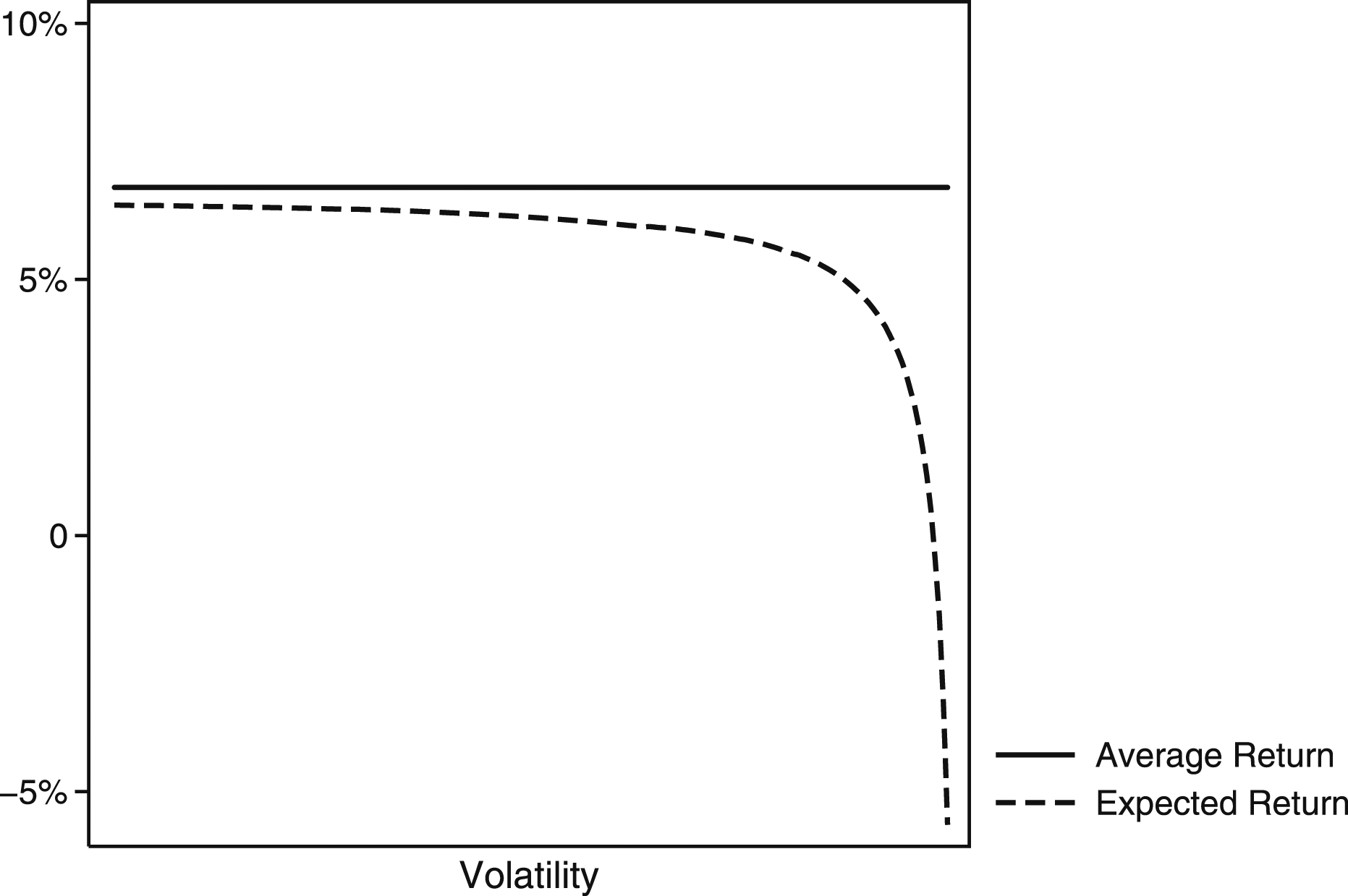
The intuition about this conclusion relates to the compounding effects of asset returns over time. Put simply, asset returns are related to each other in that future returns depend on the past, and high volatility in one period will reduce what investors can expect to earn in the future. Thus, even if risky assets such as stocks produce greater returns over time than safer assets such as real estate do, there will be periods when the expected returns on financial assets fall sharply. Neglecting market risk does not present a problem as long as there is low to moderate volatility in the market. However, as the level of risk rises, expected returns can start to deviate from observed returns in general. Increased volatility can cause problems when we compare individuals based on their current asset holdings. Instead, we should expect different effects, especially of the possession of financial assets between elections (given the variation in expected returns).
To illustrate how market risk influences voting, we can imagine a world where there are two parties competing for the votes of asset owners. Once they are elected, these parties promise that they will implement differing policies and reforms. The right-wing party, on the one hand, promises a low-tax scheme and a trimmed welfare state, thereby benefiting businesses and shareholders. The left-wing party, on the other hand, promises to benefit the less well-off with expanded welfare benefits financed by a higher tax rate. And given the self-interested voters, elections, in this world, often become about the general tax rate.
Thus, when will asset owners vote for the right-wing policy platform? Well, citizens must decide on whether to vote for a high or a low tax rate, based on both their current financial status and their future expectations. With a simple formal model, it can be shown that an individual’s marginal benefit from a higher tax rate falls with higher average returns, but rises with a higher level of market risk. Please see the Appendix for mathematical proofs. More precisely, I use a setup similar to Ansell’s (2014) to show that asset owners have more use for welfare spending when the level of market risk rises, given the negative relationship between expected returns and market uncertainty.
Furthermore, self-interested asset owners should only vote for the right-wing party if the expected benefit from right-wing policies is greater than that of left-wing ones. This condition may be fulfilled during long periods when asset returns remain stable. However, voting becomes much harder in a world where citizens must identify potential risks in advance, analyze these risks, and take action to protect their financial status. During periods marked by sharp spikes in market risk, for instance, asset owners can become indifferent between the opposed policy platforms—or even, in fact, supportive of the left, given a drastic fall in expected returns. Hence, I hypothesize based on this background that: the electoral support for right-wing parties decreases when the level of market risk increases.
This prediction is similar to what many studies have found: namely, that economic insecurity leads to support for left-wing policies (Cusack et al., 2006; Rehm et al., 2012; Rehm, 2011; Milita et al., 2019; Vlandas, 2019). Sharp increases in financial market risk, in this view, can serve to reduce electoral support for parties with a traditional right-wing profile, thereby generating cycles in patrimonial voting over time. Asset owners flock toward conservative parties when risk in the market is low, but they move closer to the center or even the left when the risk level is high.
Institutional Setting and Dependent Variable
The main issue we confront when estimating the impact from risks on voting is that assets are not randomly distributed across the population. A very strong selection process operates instead, whereby citizens with a tolerance for risk accumulate riskier assets over time, while risk-averse persons invest in assets with lower risk profiles. The problem is that both risk profiles and investment choices correlate with political preferences. Left-wing voters, for example, invest in financial assets to a lesser degree (Kaustia & Torstila, 2011). We find the same pattern in lottery studies if we collate the demand for lottery tickets with risk preferences because such preferences too are linked to voting choices (Lin˜eira & Henderson, 2019). Studies that manage to control for such factors report very weak effects from assets on voting (Ahlskog & Brännlund, 2021).
To mitigate selection problems, we can introduce panel data. To the best of my knowledge, however, this is rarely available at the individual level, unfortunately. My solution, therefore, is to look for both spatial and temporal differences across electoral districts. These districts cover very small areas in Sweden, and they usually contain some 1000 to 3000 voters. They are nested, furthermore, within municipalities ruled by a local government. There are 290 local governments in Sweden, all elected on the same day as the election for the national parliament.
It is common to treat local elections as something similar to national ones. In fact, it has been argued, Swedish municipalities operate in a quasi-parliamentary fashion, in that the mayor and the committee chairs are appointed by the coalition that wins a majority on the local council. In this setting, the largest coalition has a significant influence on local policy, and the formation of the local government is similar to that which takes place in many other systems based on proportional representation (Bäck, 2003; Cronert & Nyman, 2020). Hence, election results in the aforementioned districts decide the political coloration of the local government. Moreover, two thirds of all social services in Sweden are provided by these local governments, making these elections important.
There are local parties, but local branches of the parties represented in the national parliament tend to dominate. This implies there is a clear left/right dimension to local politics as well. This division is important because the ideology of the parties in power has a reported effect on local redistribution. Even if all local governments are obliged to provide public goods and services, left-wing governments tax and spend 2 to 3% more than do their right-wing counterparts, and they employ 4% more workers (Pettersson-Lidbom, 2008). These services are financed by grants from the Swedish government and by a proportional local income tax. Due to its clear left/right dimension, then, the Swedish system of municipalities has often been treated as a bipartisan two-party system in empirical research (Alesina et al., 1997; Pettersson-Lidbom, 2008).
Local governments have two especially interesting aspects that suit this study. First, their ability to tax assets is limited. This is important because asset taxation was a highly debated topic in Swedish politics during the period under study. The taxes on wealth and on property, respectively, were abolished in 2007 and 2008 by the right-wing government, and the left-wing opposition reacted by promising in the upcoming election to reinstate such taxes.
This question of asset taxation makes Swedish national elections a most likely case for finding an effect from assets in general, since such taxation generates a clear political conflict. More precisely, as Hellwig & McAllister (2019) illustrated recently, the degree of policy divergence between the parties is crucial for the patrimonial vote, in that the effect thereof only appears when parties position themselves far away from each other on taxes in the policy space. Focusing on local governments allows me to study the effects from market risks in a more neutral setting.
Another advantage with looking at local government is that there is partisan diversity among ruling incumbents. That is, some municipalities are ruled by right-wing parties; others are ruled by the left. This diversity is important because previous research has found that voters use asset markets as a cue for casting a sociotropic vote. More precisely, citizens vote for the government when asset prices rise, but turn to the opposition when they fall (Larsen et al., 2019; Ostrom. et al., 2018; Prechter et al., 2012; Fauvelle-Aymar & Stegmaier, 2013). However, variation in government partisanship allows me to separate policy from incumbent based voting.
Hence, the main dependent variable in this study is the change in the share of votes obtained by the right-wing bloc in each electoral district i. I register a right-wing vote when an individual votes for the Moderate Party, the Centre Party, the Liberal Party, or the Christian Democrats.
1
The clear left/right divide between the political blocs on economic policy is further explained and visualized in the Appendix. Hence, I expect to find falling support for the right-wing bloc when the degree of market risk increases. Figure 2 shows the distribution of changes in the dependent variable. The distribution of change in support for the right-wing parties over time across the electoral districts 2002–2014.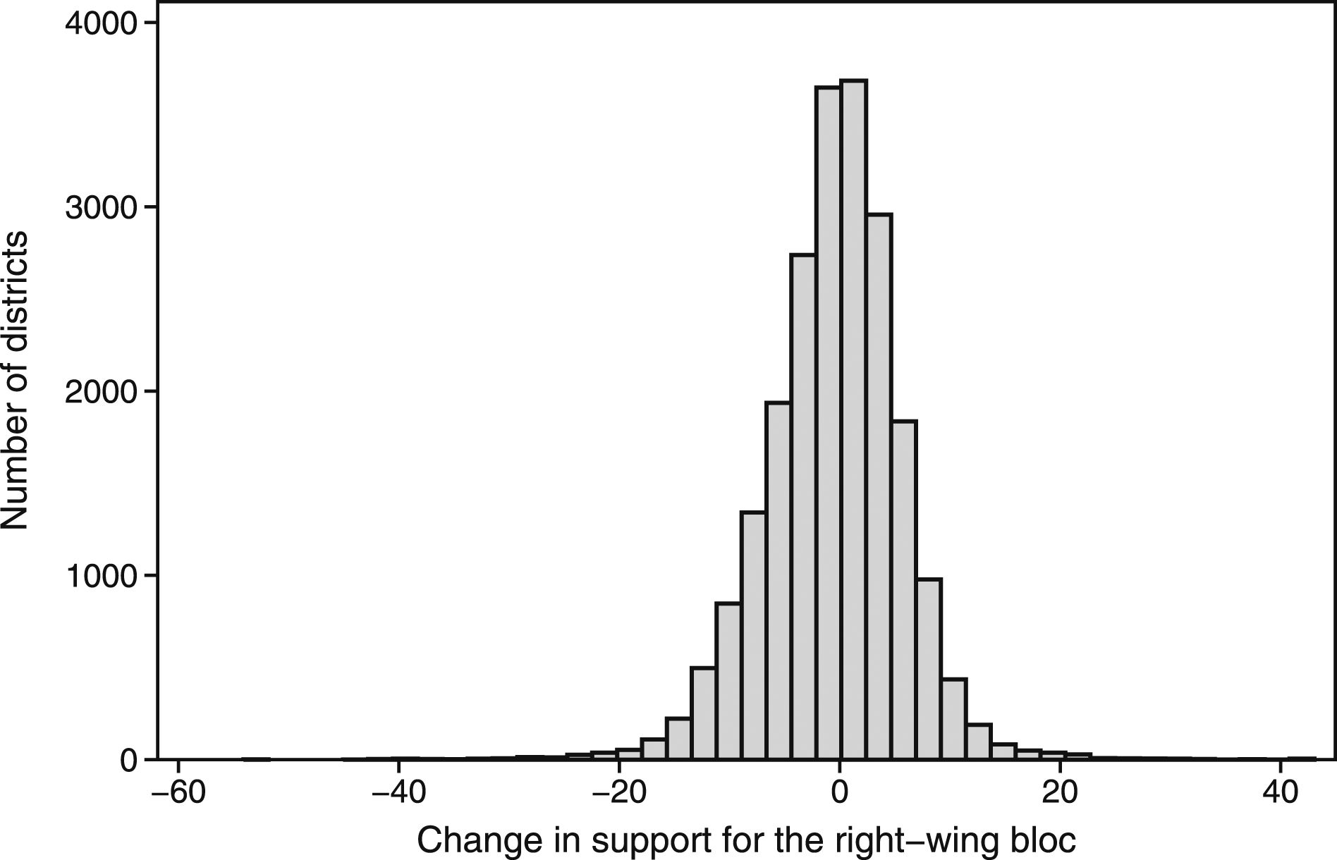
Independent Variable
My empirical strategy draws inspiration from the approach applied in studies of labor-market risks, especially those that find a relationship between labor-market risk exposure and support for welfare spending (Cusack et al., 2006; Helgason & Mérola, 2017; Milita et al., 2019; Rehm et al., 2012; Vlandas, 2019). According to the authors of these studies, occupational unemployment is a good way to measure exposure to labor-market risks and income shortfalls. That is, all citizens can act on changes in the business cycle, but those who are about to lose their job will act with policy in mind, rather than just punishing the party in charge (Helgason & Mérola, 2017). I will adopt a similar approach here since those who own a large share of financial assets should have a greater exposure to financial-market risks. That is, all individuals can act on changes in asset prices, but those who are about to lose money will act with policy in mind.
Moreover, the literature on patrimonial voting draws a clear dividing line between risky and less risky patrimony. Examples of risky patrimony are private equity, stocks, or other types of financial products (Foucault et al., 2013; Stubager et al., 2013; Lewis-Beck et al., 2013). Such assets have higher but riskier returns, and they need more active management than do less risky investments. However, financial assets are also extremely sensitive to changes in world market sentiments—especially risk and fear. A common way of measuring such market risk is with the Chicago Board Options Exchange Volatility Index, more commonly known as VIX. The VIX measures forward-looking expectations regarding volatility among world investors. It rises when investors expect large volatility in US markets. The path of the VIX index can be seen in Figure 3. The path of the VIX-index over time. The shaded areas are the months of each election.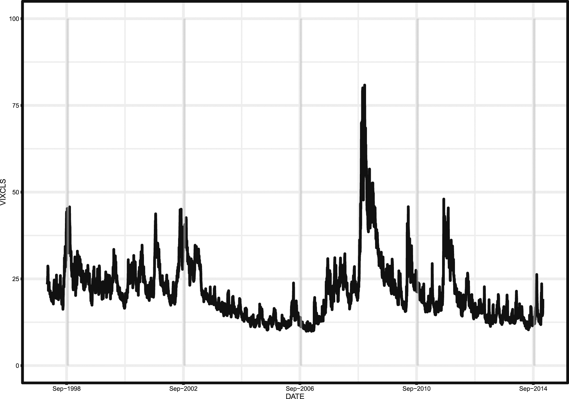
The VIX is often referred to as the index of fear. A high VIX level—80, say—would be seen in something like the 2008 financial crisis: that is, a complete financial meltdown. Under such high levels of stress, investors often abandon riskier assets such as stocks in favor of safer ones like government bonds. A low index level, on the other hand, indicates that markets are calm, encouraging investors to acquire riskier assets once more. This pattern is sometimes referred to as risk-on, risk-off behavior. Still, the problem is that sharp spikes in the VIX index often come without warning. Figure 3 suggests that, over long periods of time, the market can yield stable returns—that is, financial assets are stable investments. But market sentiments can change fast, leaving investors in a state of panic.
Initially, for instance, there was immense uncertainty around the time of the dot-com bubble, in the early 2000s. This was a major bust in the stock market, and it affected most owners of financial assets. However, the really sharp spikes came in the aftermath of the global financial crisis of 2008. The rest of the shock was brought on by the collapse of Lehman Brothers and the meltdown in US mortgage markets. Other spikes followed in 2010 and 2011, reflecting financial distress over the sovereign-debt crisis in Europe. Most investors were simply caught off guard by these spikes and were unable to diversify into less volatile assets in time.
Such surprises are painful for asset owners, but they have an advantage for purposes of analysis. That is, they allow us to identify the effect from market risks on voting. Arguably, that is to say, those who hold a large share of financial wealth will be affected more heavily by spikes in the VIX index than will those with smaller holdings. Consider the following specification:

I define market-risk exposure as the total value of risky assets in district i during the year 1999, divided by the value of total assets in the same district, multiplied by the change in the VIX index in period t, where t = (2002, 2006, 2010, 2014). More precisely, I define stock holdings and mutual funds shares as risky assets, as seen in the literature on patrimonial voting (Foucault et al., 2013; Stubager et al., 2013; Lewis-Beck et al., 2013). Total assets are constituted by housing and apartment wealth, plus these risky assets. These data are provided by Statistics Sweden, and the total value of each asset class has been generated from the Swedish Wealth Register. However, data are only available for the years 1999 through 2006, since the Swedish Wealth Register disappeared in 2007 in connection with the abolition of the wealth tax. The risky-to-total-assets ratio across the districts is visualized in Figure 4. The distribution the risky-to-total asset ratio across electoral districts.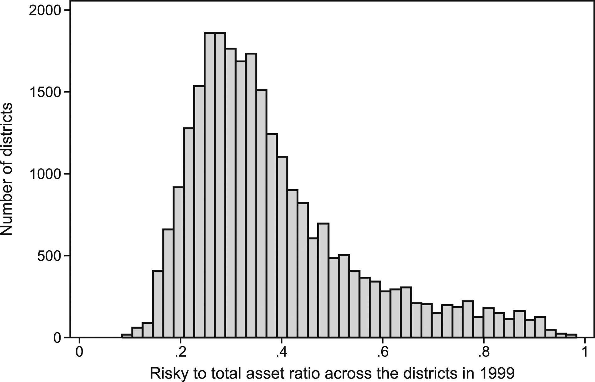
As we can see, most districts have fewer risky assets than non-risky ones. The most common form of asset wealth in Sweden is housing wealth; few households have a large portfolio of stocks. However, most households do save in mutual-funds shares—a behavior which has exposed many savers to financial risks. So, by multiplying changes in the VIX index by their associated share of risky investments in the districts, I obtain a proxy for changes in exposure to market risks. This process bears some resemblance to a shift-share instrumental-variable design with only one share (Goldsmith-Pinkham et al., 2018). However, this is not an instrumental variable setup, since I lack both first- and second-stage equations. I look instead at the reduced-form effect from my proxy variable on election outcomes among the districts.
Empirical Specification
I identify the effect on voting from market-risk exposure by analyzing how the right-wing’s share of votes evolves in districts with high and low risky-to-total-assets ratios over time. This identification strategy has some resemblance to a reduced-form shift-share instrumental-variable strategy, where the share or the risky-to-total-assets ratio is fixed at 1999, and the time-varying shifter is changes in the VIX index. There is a trade-off here, in that fixing the share leads to greater chance of satisfying the exclusion restriction, while on the other hand reducing instrument relevance (Broxterman & Larson, 2020). Still, we need not worry so much about the exclusion restriction, given we are observing the reduced-form effect. However, another reason for fixing the share at 1999 is the relationship between partisanship and investing, because such behavior opens up for reverse causality (Kaustia & Torstila, 2011). Moreover, since I only have one share, the main identifying assumption reduces to that of a conventional difference-in-differences strategy with continuous treatment (Borusyak et al., 2018; Goldsmith-Pinkham et al., 2018). This specification presents a linear relationship between my main variables

Here, the dependent variable is support for the right-wing bloc in a local election in period t, in electoral district i, which is nested in larger municipality m. The dependent variable is expressed in differences, in order to cancel out time-invariant unobserved heterogeneity across electoral districts. The main variable of interest on the right-hand side of equation (2) is changes in district exposure to market risk: that is, the interaction term between changes in the VIX index and the risky-to-total asset ratio in district i.
Given the resemblance here to a difference-in-differences strategy, the key identifying assumption is that the average change in voting among districts with low risk ratios is equivalent to what the average change would be in districts with high risk ratios if there were no changes in the VIX index over time. Hence, districts with high and low risk ratios should be on parallel paths in voting over time. But we can never actually observe such trends, given the continuous changes in the VIX index.
To make the model less restrictive, therefore, I include a linear time trend, which in the first-difference setup translates to a district-fixed effect. By including district-fixed effects ψi, the identifying assumption shifts from parallel paths to parallel growths in voting. This is a weaker assumption, in that districts with high and low risk ratios are allowed to be on different trends in voting as long as these trends are linear (Mora & Reggio, 2012).
A crucial problem here, however, relates to regional trends in voting that vary with the regional business cycle, the political orientation, and even the size and performance of the local government. That is, I want to make sure the districts I compare have as similar pre-trends as possible from the beginning. So, a crucial addition to this setup is to interact year-fixed effects δt with a municipality dummy ζm. This simple interaction term ensures that I exploit variations across districts with different levels of risky-to-total-assets ratios within the same municipality.
Adding both spatial and temporal fixed effects restrict the identifying variation to the difference between how the de-trended support for the right-wing bloc reacts to changes in the de-trended VIX index in districts with a large share of risky assets, compared to the corresponding response in districts with low shares of risky assets within the same municipality. This model is described in the following equation

In terms of additional controls, a big concern is that the risky-to-total-assets ratio picks up important interaction between other districts’ characteristics and changes in the VIX index. To begin with, the risky-to-total-assets ratio does not reveal anything about how wealth is distributed across or within districts. This is problematic since a high ratio can be driven by the holdings of one or two super-wealthy citizens, and the impact on voting can as easily be driven by an interaction between wealth inequality and changes in market exposure. To adjust for such effects, I control for districts’ relative financial wealth against that of other districts, for wealth inequality, and for the ratio between owners and non-owners of financial assets within the districts. One problem, however, is that such data are not available over time. To solve this issue, I interact the conditions found in the districts in 1999 with a set of election dummy variables. For the exact construction of these variables, see in the Appendix.
Another concern relating to endogeneity is the changes in housing prices since such prices have been linked to changes in both policy preferences and voting (Ansell, 2014; Ansell et al., 2018; Larsen et al., 2019). Put simply, it is possible that districts with a high ratio of risky to non-risky assets suffer more in terms of falling house prices when there is more uncertainty in financial markets. So, in order to investigate whether housing prices influence the estimate, I generate a variable that captures district growth in housing prices. To create this variable, I combine growth in housing wealth for the years 2002 and 2006 with growth in housing prices for the years 2010 and 2014. To control for the effect of other economic variables, I add household income, average years of education, share of migrants, population size, age, age squared, and changes in the unemployment rate. Please see the Appendix for construction and data sources.
Finally, we must also remember that the main independent variable here—market risk exposure—is at its core an interaction term between a share and a shifter. Adding simple control variables to such a design adjusts for the linear effect from such controls, but it does not allow for a heterogeneous impact of these controls. Thus, to control for heterogeneous trends in observable confounders, I interact my time-variant controls with the share of risky assets during the base year 1999.
Results
Market Risk Exposure and Right-Wing Voting
In this section, I evaluate the main argument in this study: that right-wing parties lose support on average when the level of market-risk exposure increases among asset-owners. The dependent variable is changes in the voting share of the right-wing bloc in electoral districts in local elections in Sweden. The main independent variable—market-risk exposure—is an interaction term between the changes in the VIX index and the ratio of risky to total assets at the district level. Regarding the functional form, I investigate the non-parametric relationship between visual changes in market-risk exposure and changes in right-wing voting in the Appendix. The visual relationship between these variables is approximately linear.
Market Risk Exposure and Right-Wing Voting.
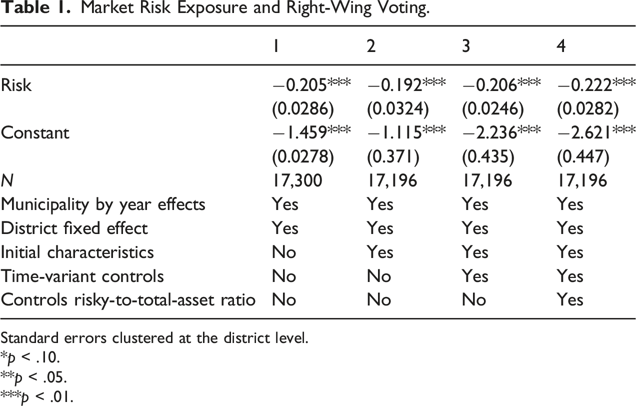
Standard errors clustered at the district level.
*p < .10.
**p < .05.
***p < .01.
However, since these characteristics are time-invariant and will get soaked up by the fixed effect, I interact them with a time dummy in each period. Thus, I can control for periodic shocks across districts with high or low inequality, with a strong or weak position in the national wealth distribution, and with differing degrees of financial ownership. Adding such controls reduces the estimate to −0.19. The next step is to investigate whether time-variant controls such as changes in economic and demographic characteristics over time have an impact. I do this in column three. It increases the estimate to −0.21. As a final test, however, I allow for an interaction between these observables and the risk ratio in 1999. This estimate is presented in column 4. As we can see, it is marginally stronger, at −0.22.
These estimates give little indication that either observed or unobserved heterogeneity which grows over time in a linear fashion presents a problem. However, one can certainly push the tests further. For instance, I include district-fixed effects in the main model, which is the same as netting out long-run linear trends in voting. This is the first estimate presented in Figure 5. However, more steps can be taken to get rid of unobserved heterogeneity across electoral districts. One way is to multiply the district-fixed effect by a linear time trend. This is the same as controlling for long-run quadratic trends in voting or for unobserved confounders that grow over time in a quadratic manner. Testing for pre-trends in voting.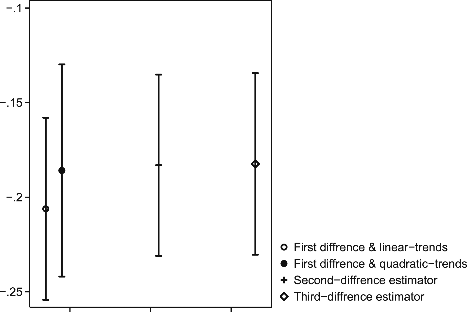
The results from such a flexible function can be seen in Figure 5 as well. More precisely, this specification is represented by the second coefficient from the left. One possible problem with this design, however, is that the trends must be consistently estimated since inconsistently estimated trends will add bias to the model. In the end, I have very few years on which to estimate such trends. Still, there are simpler ways of de-trending variables, such as by looking at the second- and third-difference estimates. I, therefore, run two additional regressions, where I look at the relationship between the second- and the third-difference transformation of these variables. This transformation implies that I look at correlations between the accelerations in voting and market risk, and the rate of change in these accelerations, which arguably should include fewer traces of trends compared to plain changes. The results, presented in Figure 5, are very similar as well.
Market Risk Exposure and Party Voting
The purpose of this section is to investigate what types of parties gain or lose support when voters are exposed to market risk. Hence, I simply break down the results on individual parties and I present the estimates in approximate left/right order based on the Chapel Hill Expert Study. Please see the Appendix. It follows from my argument that no right-wing party should benefit from higher market-risk exposure. It follows too that parties to the left should gain support, given that they offer more generous redistribution plans (Figure 6). Individual regression coefficients for the effect from asset risk on the political parties in the following order: Left Party (LP), Social Democratic Party(SDP), Green Party (GP), Christian Democrats (CD), Center Party (CP), Liberal Party (LP) and Moderate Party (MP).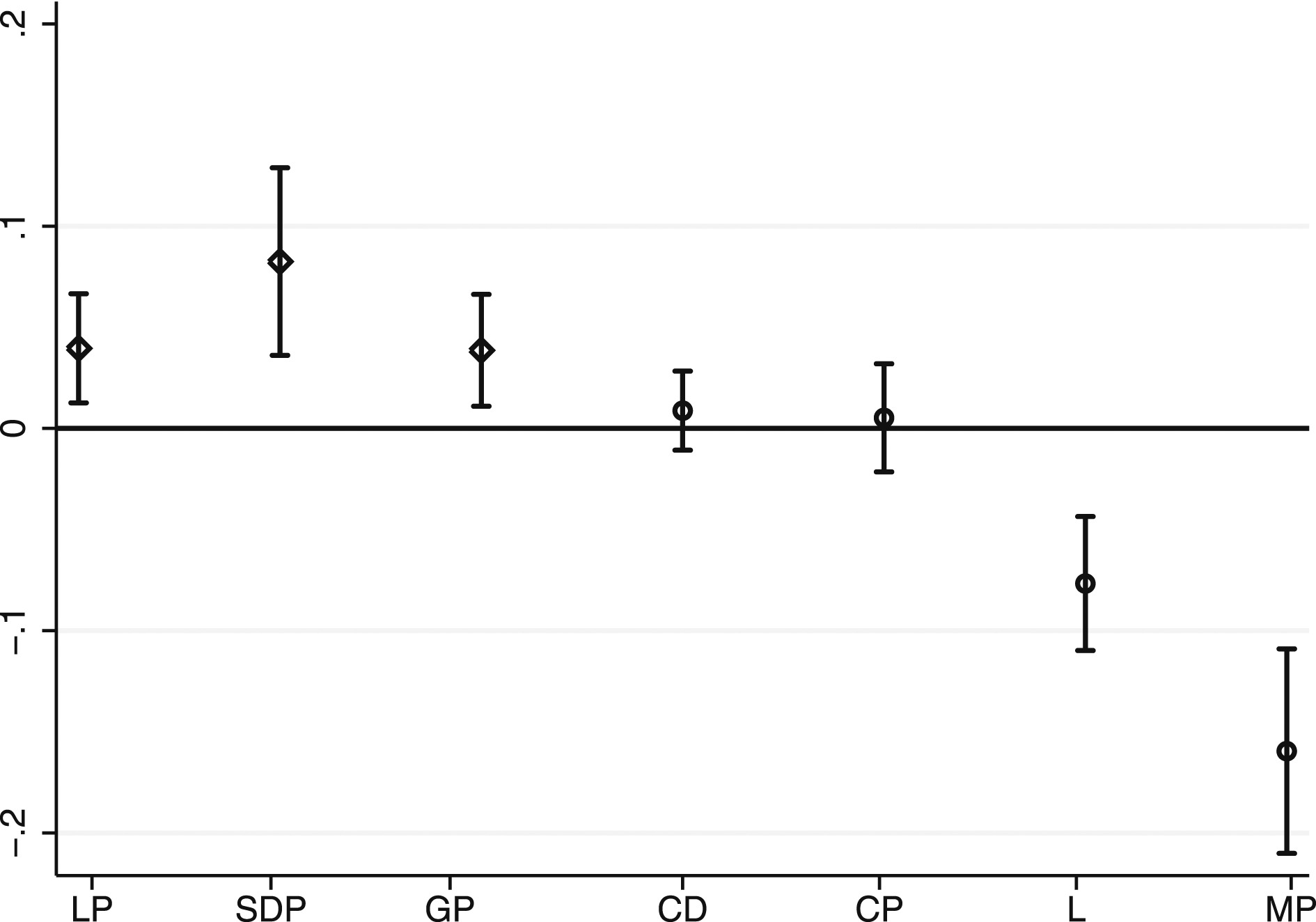
The results suggest that all three left-wing parties—the Left Party (LP), the Social Democrats (SDP), and the Green Party (GP)—benefit from rising asset risk. On the other hand, there are only two clear losers in the right-wing bloc from increased asset risk: the Liberal Party (LP) and the Moderate Party (MP), which at the time were the two parties with very clear pro-market platforms. The Moderate Party is the largest party in the right-wing bloc, and the main challenger to the Social Democrats. In contrast, two smaller right-wing parties—the Centre Party (CP) and the Christian Democrats (CD)—do not seem to suffer much. In sum, these individual estimates suggest that left-wing parties gain momentum from asset risk, while two right-wing parties suffer.
Market Risk Exposure and Incumbency Voting
The purpose of this section is to investigate whether the effects are conditional on incumbency. An important part of my argument is that voters act prospectively rather than retrospectively—that is, that they choose political parties based on the expected value yielded by their policy platforms. This restriction is problematic, inasmuch as a well-established argument in political science is that citizens reward or punish politicians according to their assessment of current economic conditions. More precisely, the sociotropic-voting hypothesis states that citizens rally behind the sitting government when the economy performs well, and that they opt for the opposition when the economy is in recession (see, for instance, Kiewiet & Lewis-Beck, 2011).
Fluctuations in asset valuations, from this perspective, can influence citizens through a similar mechanism, given that some studies indicate stock-market gains are correlated with presidential approval in the US (Fauvelle-Aymar & Stegmaier, 2013; Ostrom et al., 2018; Prechter et al., 2012), and with satisfaction with the government in the UK (Key & Donovan, 2017). Even housing prices are said to correlate with the incumbent vote (Larsen et al., 2019). The problem is that changes in the VIX index will correlate both with large swings in prices for multiple asset classes and with the wider business cycle. Thus, it becomes hard to separate the impact of market risk from that of retrospective behavior if voters are allowed to act on both. Hence, to toughen up the test further, I investigate whether the effects are conditional on incumbency, as seen in Figure 7. The coefficients are presented in the following order: the effect on all governments, the effect on left-wing parties under a left-wing government and left-wing parties under a right-wing government, right-wing parties under a right-wing government, and right-wing parties under a left-wing government.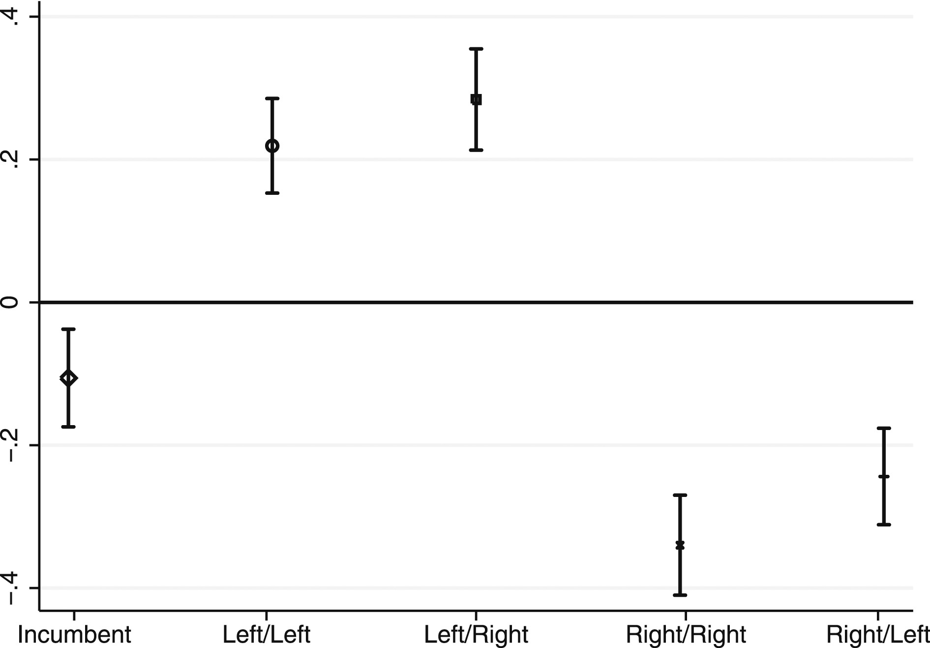
The first coefficient presents the effect from market-risk exposure on all governments. As can be seen, this effect is negative. Such an effect suggests that voters can behave in a retrospective manner and punish all governments for increased risk exposure. If we break down this result, however, we see first that left-wing parties enjoy higher support, both in government and in opposition. Right-wing parties, on the other hand, seem to lose support from increased asset risk, at all times.
Additional Specifications
The attentive reader may be worried that the effect is heterogeneous across districts with high and low ratios of ownership shares since the independent variable is derived from asset values rather than from the number of owners. Perhaps we should expect to find different types of effects in districts where financial wealth is concentrated in just a few hands than in districts where we find a more even distribution. To investigate any concerns over this, I run an alternative analysis in the Appendix, where I look at the impact from market-risk exposure per owner. That is, I weigh the main independent variable by the share of owners in each district. Such an analysis does not, however, tell a different story.
Another concern pertains to standard errors. The unit of observation is a district election, and the standard errors are clustered by district. However, it is easy to imagine that districts with similar mixes of stocks and mutual-fund shares are subject to idiosyncratic shocks in voting. Suppose, for example, that young, urban districts with less financial wealth shifted toward a particular party in one election because they liked its policy offerings, and that, unrelatedly, the VIX value changed sharply in that same election. It would look as if market-risk exposure had affected the voting, and the estimate would furthermore be highly significant statistically. Yet, it would be a statistical artifact (see Adão et al., 2019, for more discussions of these concerns). To correct for this problem, I follow Adão et al. (2019) and run tests where I cluster the standard errors on how similar the districts are in terms of risky to total assets ratios in the Appendix. These tests are not different from the main results.
Discussion
Many scholars have suggested that wealth, especially in the form of risky patrimony, increases support for traditional free-market parties because holders of financial assets have more to gain from right-wing policies (Foucault et al., 2013; Stubager et al., 2013; Lewis-Beck et al., 2013). However, the application of more quasi-experimental research designs has called into question the casual impact of economic affluence on economic-policy preferences and thus the validity of this relationship. To shed light on this inconsistency, I have sought to explore the role of market risk in asset ownership to show that right-wing parties suffer when market risk rises. Thus, I argue, holders of financial assets become less tempted by free-market policy offerings when there is great uncertainty in financial markets.
The general idea in the literature on patrimonial voting is that investors handle risks through asset diversification. Those who accept higher risks take on financial assets; those who prefer to play it safe invest in less volatile assets, such as real estate. The problem, however, is that owners of assets also become exposed to market risks that change between elections. That is, markets can be calm for long periods of time and can generate stable asset returns but can—suddenly and with little warning—fall massively. The world has witnessed huge financial shocks of such a pattern in recent decades. The dot-com bubble, the financial crisis, and, most recently, the coronavirus’s massive impact on financial markets show that people’s savings can evaporate in a matter of days. It is not clear, therefore, why citizens who invest money in the market would support right-wing parties at all times.
My empirical strategy has some resemblance to the shift-share IV design, but the problem is that I have no real measures of perceived market risk among voters. This leaves me with a reduced-form effect. From one standpoint, this is not very strange, as it is common to draw conclusions from reduced-form estimates with a shift-share design (Goldsmith-Pinkham et al., 2018). However, the lack of a first stage limits my ability to draw any conclusions regarding the size of the market risk’s effects. The problem is that changes in the VIX index, along with the share of financial assets, can constitute an effective instrument for perceived market risk among investors; however, these do not work as a perfect proxy for such risks on their own.
Still, one way to get a sense of the size of these effects is to compare the impact of an increase in the VIX index on voting across districts with different shares of financial assets. For instance, the average share of financial wealth in the districts is 0.4, while the share in districts with zero financial wealth is 0. This difference means that the local right-wing bloc gain/loses, on average, 0.08 (0.4*0.2) percentage points in support in the typical district compared to districts with no financial wealth after a one-point decrease/increase in the VIX index. This effect seems small but should be seen in relation to the large shifts in the VIX index observed in Figure 3. In fact, the sharp decline in the VIX index (−15) between the election in 2002 and 2006 coincide with the victory of the right-wing parties in many municipalities as well as with the victory of the right-wing bloc in the national election. The left-wing bloc on the other hand, lost the election in 46 municipalities but the average margin between blocs where only 1.5 percentage points across the electoral districts.
Furthermore, I aim no critique at the argument made in the literature on patrimonial voting. My purpose has instead been to nuance these arguments, by showing that expected returns and changes in market risk matter as well. That is, voters are far more complex than we had previously believed in the models of patrimonial voting. For instance, voters who become wealthy from rising asset values can simultaneously become fearful of future losses if there is uncertainty in the market. Such uncertainty can decrease support for right-wing parties even if asset prices rise. Free-market policies and a slimmed-down welfare state can seem appealing to asset owners most of the time. However, under conditions of extreme market uncertainty, such policies can become expensive. Political scientists ought, therefore, to start thinking about asset wealth in terms of both risks and rewards.
The final question is how far can these results travel? This is a tricky question because one can make the case for both a relatively stronger and weaker effect in this institutional setting. To begin with, I study these effects in local elections and politicians at this level do not influence financial markets or financial regulation. Voters are instead more likely to select local politicians based on their demand for local welfare services. Hence, local elections constitute a good testing ground for my hypothesis, but the effect can, at the same time, be smaller in the general elections because voters vote based on macro-economic performance as well as asset taxation in these settings. More precisely, the effects of patrimony on voting are likely to be smaller in the local context since asset owners are more likely to move to the right when there is polarization between political parties on important economic issues (see Hellwig & McAllister, 2019).
One can, on the other hand, make the case for a stronger impact on left–right voting in Sweden because voters are more likely to vote based on economic policy preferences rather than the macro-economy in mature democracies (Quinlan & Okolikj, 2020). However, Sweden is also known for its egalitarian welfare-state policies and for its even income distribution, and this context constitutes an arduous test for economic voting and, particularly, a wealth-based hypothesis. This is because a larger effect of asset wealth on voting has been found in more liberal welfare systems such as the UK and in countries where the tax system does not limit citizens to invest (Quinlan & Okolikj, 2019). Still, although Sweden has among the highest marginal taxes on income, it treats wealthy asset owners in a very different manner.
During the studied period, the Swedish wealth and property tax was abolished in 2007 and 2008, respectively, by the right-wing government. The social democratic government, on the other hand, abolished both taxes on inheritance and gifts during the preceding period. Government revenues from capital income further declined after the introduction of a special account in 2012 for financial savings; furthermore, corporate taxes were lowered in several steps. Sweden is, in other words, a generous welfare state but it encourages at the same time citizens to save and invest in assets.
Finally, asset wealth is often less evenly distributed than labor income in most economies, and this is true for Sweden as well. The median citizen today has less than half the savings of the average citizen, indicating that a small group with large savings pushes the average higher, while a typical Swede has considerably less savings. One explanation behind this pattern is that a significant share of all wealth in Sweden is inherited, up to 50% of all private wealth according to some estimates (Ohlsson et al., 2019). Today, 10% of the wealthiest households own 75% of all wealth, and the common Swede has very little assets in comparison to citizens in other OECD nations. In fact, the median voter in Sweden is among the poorest in Western Europe when it comes to asset wealth. 2 Thus, we would expect a relatively smaller effect in Sweden given the modest holdings of financial wealth. To conclude this discussion, one can make different arguments about the Swedish setting, and future works should, consequently, make similar studies and investigate this effect on the comparative level.
Footnotes
Acknowledgment
I am grateful for the helpful comments from Karl-Oskar Lindgren, Pär Nyman, Linuz Aggeborn, Marcus Österman, Adrian Adermon, and two anonymous reviewers.
Declaration of Conflicting Interests
The author(s) declared no potential conflicts of interest with respect to the research, authorship, and/or publication of this article.
Funding
The author(s) disclosed receipt of the following financial support for the research, authorship, and/or publication of this article: This study was partly financed by the Swedish Research Council (Grant Number 2017–0076,4).