A quasi-Bayesian Approach to Small Area Estimation Using Spatial Models

Abstract

The empirical best linear unbiased prediction (EBLUP) method has been the dominant model-based approach in small area estimation. As an alternative to this frequentist method, the observed best prediction (OBP) method, also frequentist, was proposed by Jiang et al.^[11] where the parameters of the model are estimated by minimizing an objective function which is implied by the total mean squared prediction error. In a recent article, Datta et al.^[6] followed a general Bayesian approach, proposed recently by Bissiri et al.^[2], to develop a quasi-Bayesian method by appropriately calibrating the objective function for the OBP method for the Fay-Herriot model. In a different article, Chung and Datta^[4] demonstrated that in the absence of covariates with good predictive power the small area estimates from the standard Fay-Herriot model can be improved by using spatially dependent random effects. In this article, we develop a quasi-Bayesian small area estimation method using several spatial alternatives to the independent Fay-Herriot random effects model. Evaluation of the proposed method based on an application to estimation of four-person family median incomes for the U.S. states shows its usefulness. Limited but related simulation studies for the median incomes application reinforce our conclusion.

AMS Subject Classification: 62F15, 62D99

1. Introduction

Shrinkage estimation of the mean vector $\left({\theta }_1,\cdots ,{\theta }_m\right)$ of a multivariate normal distribution is a pioneering breakthrough in statistics by Stein^[21]. He showed that the vector of shrinkage estimators of the individual means has lower frequentist risk under a sum of squared error loss than that of the uniformly minimum variance unbiased estimator vector. Shrinkage estimation makes sense when the components of the mean vector have similar interpretation such as means of a characteristic for many similar subpopulations. Concurrent estimation of subpopulation means is of fundamental importance in small area estimation. Small areas in survey sampling are subpopulations, defined by demographic and/or geographic partitioning of a suitable population. Small areas are actually subpopulations or subdomains of some target population which do not get enough allocations of samples to estimate their means with adequate accuracy.

In a pioneering paper, Efron and Morris^[8] showed Stein’s estimators can be interpreted as empirical Bayes (EB) estimators of the means if one assumes some appropriate models for the mean vector. This EB representation presents a heuristic justification for the above-mentioned risk domination that shrinkage estimators enjoy.

Reliable estimates of subpopulation characteristics ${\theta }_i\text{ s}$ are urgently needed by many national statistical offices to help government administrators implement various social and fiscal policies of their governments. However, a traditional estimate $Y_i$ , also called a direct estimate, of ${\theta }_i$ based only on the sample from that subpopulation may have unacceptable level of estimation error if the corresponding sample size is small. To improve low accuracy of direct estimates of small area means, researchers recommended combining information from the other subpopulations, possibly similar, through model-based estimation of small area means by using suitable models for the ${\theta }_i$ s based on appropriate covariates, if available.

In a large-scale pioneering application of model based small area estimation of average incomes of many small localities in US, Fay and Herriot^[9] proposed a model which is now extensively used in small area estimation. Their model, which is known as the Fay-Herriot model in small area estimation literature, implicitly connects direct estimator $Y_i$ of ${\theta }_i$ with related covariates $x_i$ .

Fay and Herriot^[9] proposed a mixed effects model given by

$$Y_i={\theta }_i+e_i,{\theta }_i=x_i^T\beta +v_i,i=1,\dots ,m,$$

(1.1)

where $Y_i$ is related to ${\theta }_i$ via the sampling model, and ${\theta }_i$ is related to the covariates $x_i$ via the linking model. It assumes that the sampling error $e_i$ satisfies $E_P\left(e_i\mid x_i\right)=0$ and $V_P\left(e_i\mid x_i\right)=D_i$ , where the subscript $P$ refers to the sampling design. Sampling errors are assumed to be independent and normally distributed, and are independent of linking errors, $v_i$ , the area-specific random effects, which are assumed to be independent and normally distributed with zero mean and a common variance $A$ . The sampling variances, $D_i$ ’s, which are usually estimated, are treated as known. We denote model parameters ${\left({\beta }^T,A\right)}^T$ by $\psi$ , where $\beta$ is a $p\times 1$ vector of unknown regression coefficients. In the FayHerriot model, for a $p\times 1$ vector of known covariates $x_i$ , estimation of small area means becomes prediction of the mixed effects ${\theta }_i=x_i^{\top }\beta +v_i,i=1,\dots ,m$ .

While Fay and Herriot^[9] used the EB approach to estimate ${\theta }_i$ based on the model given by equation (1.1), Prasad and RaO^[15], Lahiri and RaO^[12], Datta and Lahiri^[5] and Datta et al.^[7] used the empirical best linear unbiased predictor (EBLUP) method, a frequentist approach, and they derived the second-order approximate mean squared error (MSE) of the EBLUPs of ${\theta }_i$ , and second-order approximate unbiased estimators of the MSE’s for various estimators of the variance parameter (see Datta and Lahiri^[5]). However, Ghosh^[10] developed hierarchical Bayes (HB) estimation of ${\theta }_i$ by augmenting the model in equation (1.1) by an improper uniform prior for $\beta$ and $A$ . Later on, Datta et al.^[7] also considered the HB prediction of ${\theta }_i$ ’s for the Fay-Herriot model.

The model in equation (1.1) assumes independence of the random effects terms $v_i$ ’s across small areas. For subsequent reference we will call this model as the independent Fay-Herriot model. Small area means of geographic areas often display a strong spatial dependence among themselves. In the absence of effective covariates, there maybe a systematic model misspecification by the independent FH model for the means due to spatial correlation among random effects. In such applications, it is recommended to use suitable spatial models for the random effects. In a recent article, Chung and Datta^[4] developed comprehensive $\text{HB}$ estimation of ${\theta }_i$ ’s under many popular spatial models based on certain noninformative priors on the model parameters. We briefly describe these spatial models in the next section.

The EBLUP approach played a major role in small area estimation (cf. Battese et al.^[1]; Prasad and RaO^[15]). While the independent $\text{FH}$ model has been a very popular model for creating the EBLUPs of small area means, many authors in the last twenty years alternatively used spatial random effects models. See, for example, Saei and Chambers^[19], Singh et al.^[20], Petrucci and Salvati^[14], Pratesi and Salvati^[17] and Pratesi et al.^[16].

The EBLUP or the EB predictions of small area means are carried out in two steps, and these predictors are derived under the popular sum of squared error loss function. For simplicity, we present the main ideas below for the independent FH model. First, for known model parameters $\psi$ , the best predictor (BP) ${\tilde{\theta }}_{i,B}$ of ${\theta }_i$ , given by

$${\tilde{\theta }}_{i,B}=Y_i-{\gamma }_i\left(Y_i-x_i^{\top }\beta \right),$$

(1.2)

is derived, where ${\gamma }_i=D_i/\left(D_i+A\right)$ . However, since $\psi$ is unknown, the predictor ${\tilde{\theta }}_{i,B}$ cannot be used. Estimators of $A$ and the regression coefficient $\beta$ are typically obtained by iterative computation based on the marginal distribution of the data.

In a pioneering paper, Jiang et al.^[11] argued that the second step in developing the EBLUPs is not suitable for prediction of ${\theta }_i$ since areas with less accurate $Y_i$ ’s have less influence in determining the model parameters. The maximum likelihood or weighted least squares estimator of $\beta$ assigns relatively lower weights to direct estimators $Y_i$ with larger sampling error variances $D_i$ ’s. Since prediction of ${\theta }_i$ ’s is the main interest, they argued for a purely predictive procedure where both the predictor of $\theta$ and the estimators of model parameters are derived by minimization of a total predictive mean squared error. We review their method in the next section. These authors also argued that their proposal, which they called observed best prediction (OBP), an alternative to the EBLUP, is less sensitive to misspecification of the mean function. Since both the spatial random effects model and the OBP method are effective tools to address misspecification of the mean function of ${\theta }_i$ ’s, in this article we develop a method by combining these two ideas. To address this objective we will extend a quasi-Bayesian method recently developed by Datta et al.^[6]. This method allows us to compute meaningful measure of uncertainty for the Bayesian analogs of OBP estimates for the spatial models. Asymptotically justified estimator of mean squared error of OBP predictor has been derived by Liu et al.^[13] for the independent Fay-Herriot model. This derivation is non-trivial, and no such results exist nor can be easily derived for the spatial Fay-Herriot models. Moreover, such estimator may not always be positive. Our proposed measure of uncertainty, quasi-Bayesian posterior variance, is computational and nonnegative. We showed in Datta et al.^[6] that the quasi-Bayesian method for the independent Fay-Herriot setup is a competitive alternative to the OBP method.

2. A Brief Review of the OBP Method

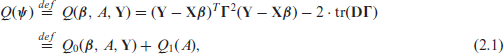
We use the notation $\theta ={\left({\theta }_1,\cdots ,{\theta }_m\right)}^T$ to denote the mean vector and $Y={\left(Y_1,\cdots ,Y_m\right)}^T$ to denote the vector of direct estimates. We first review the objective function crucial to the OBP method of Jiang et al.^[11] for the independent Fay-Herriot model. Under the sum of squared error loss function $L\left(\hat{\theta },\theta \right)={\sum }_{i=1}^m{\left({\hat{\theta }}_i-{\theta }_i\right)}^2$ to estimate $\theta$ by an estimator $\hat{\theta }$ , (Rao and Molina^[18], p. 166) presented an alternative and transparent derivation of the objective function obtained by Jiang et al.^[11] to estimate the model parameters $\psi$ . (Rao and Molina^[18], p. 166) computed the total sampling MSE of ${\tilde{\theta }}_{i,B},i=1,\cdots ,m,{\text{MSE}}_P\left({\tilde{\theta }}_B\right)={\sum }_{i=1}^m{E}_P{\left[{\tilde{\theta }}_{i,B}-{\theta }_i\right]}^2$ . Using equation (6.4.52) in their book, they obtained ${\text{MSE}}_P\left({\tilde{\theta }}_B\right)=E_P\left[{\sum }_{i=1}^m\left\{{\gamma }_i^2{\left(Y_i-x_i^T\beta \right)}^2-2D_i{\gamma }_i+D_i\right\}\right]$ . They dropped the last term, ${\sum }_{i=1}^m{D}_i$ , which is known, to obtain the objective function of Jiang et al.^[11]. This function is given by

$$Q(\psi )\stackrel{\text{def}}{=}Q(\beta ,A,Y)={(Y-X\beta )}^T{\Gamma }^2(Y-X\beta )-2\cdot tr(D\Gamma )\stackrel{\text{def}}{=}{Q}_0(\beta ,A,Y)+Q_1(A)$$

(2.1)

where $Q_1\left(A\right)=-2\cdot \text{tr}\left(D\Gamma \right)\text{In}\left(2.1\right),X={\left[x_1,\cdots ,x_m\right]}^T$ , and $\Gamma =\text{diag}\left({\gamma }_1,\cdots ,{\gamma }_m\right)$ is the shrinkage matrix shrinking $Y$ to the regression function. The resulting estimator $\tilde{\psi }={\left({\tilde{\beta }}^T,\tilde{A}\right)}^T$ , obtained by minimizing $Q\left(\psi \right)$ , is referred to as the best predictive estimator (BPE) of $\psi$ .

The objective function in (2.1), which is valid for the independent Fay-Herriot model, has been generalized by Jiang et al.^[11] even for dependent random effects model. To allow a greater generality for random effects distribution we use the precision matrix to denote a multivariate normal pdf for random effects so that even a singular pdf can be considered. If this matrix is positive definite, it is equivalent to the inverse of the variance-covariance matrix of the random effects. We present the pdf of random effects under various spatial models considered in the next section by using the precision matrix. While the precision matrices for most spatial models are p.d., it is not so for the intrinsic autoregression (IAR) model (discussed later). If a random vector $U$ has the pdf given by

$$f_U\left(u\right)\propto \text{exp}\left[-\frac{1}{2}{(u-\mu )}^T{P}_U\left(u-\mu \right)\right]\text{ for }u,\mu \in \text{colsp}\left(P_U\right)$$

we use the notation $U\sim N\left(\mu ,P_U\right)$ . Here, the symmetric matrix $P_U$ is n.n.d. and $\text{colsp}\left(P_U\right)$ is the column space of the matrix $P_U$ . If $P_U$ is singular, then the distribution of $U$ is singular. Following equation (27) of Jiang et al.^[11] we consider the following mixed effects model

$Y=X\beta +v+e$

(2.2)

where $v$ and $e$ are independently distributed with $v\sim N\left(0,P_M\right)$ and $e\sim N\left(0,P_D\right)$ . Here, we assume that $P_D$ is known, and $P_M$ depends on a parameter vector $\delta$ . We also assume that $P_D$ is p.d., which is identical to $D^{-1}$ , where $D$ is the sampling variance-covariance matrix. Let the mixed effects that we need to predict be denoted by $\theta =X\beta +v$ . If the precision matrix $P_M$ is singular, then the distribution of $\theta$ will be singular, and in that case, we also need that $\text{colsp}\left(X\right)\subset \text{colsp}\left(P_M\right)$ . Consequently, if $\text{rank}\left(X\right)=p$ , then rank of the matrix $P_M$ is at least $p$ . We redefine the model parameter vector $\psi$ by ${\left({\beta }^T,{\delta }^T\right)}^T$ .

Considering $\delta$ known, the best predictor (BP) of $\theta$ , denoted by ${\tilde{\theta }}_B\left(\psi \right)$ , can be obtained from the distribution of $v$ and $e$ . The $\text{BP}$ is given by

$${\tilde{\theta }}_B\left(\psi \right)=Y-B\left(Y-X\beta \right),$$

(2.3)

where $B={\left(P_D+P_M\right)}^{-1}{P}_M$ . The associated measure of uncertainty, $V\left(\theta \mid \psi ,Y\right)$ , is given by $\left(P_D+\right.$ ${\left.P_M\right)}^{-1}$ . Following the argument of Rao and Molina^[18] presented above, we will derive below the equivalent expression of the objective function in (2.1) for the model given by equation (2.2). Noting that ${\tilde{\theta }}_B\left(\psi \right)-\theta =e-B\left(Y-X\beta \right)$ , it can be shown that

$$MS{E}_P\left({\tilde{\theta }}_B\right)=E_P\left[{(Y-X\beta )}^T{B}^{T}B\left(Y-X\beta \right)\right]-2E_P\left[e^{T}B\left(Y-X\beta \right)\right]+\text{tr}\left(D\right).$$

Using $E_P\left[e^{T}B\left(Y-X\beta \right)\right]=\text{tr}\left(DB\right)$ , and dropping the term $\text{tr}\left(D\right)$ , and the operator $E_P\left[\cdot \right]$ from the first term we get from the previous display the following objective function

$$Q\left(\beta ,\delta ,Y\right)\equiv Q\left(\psi ,Y\right)=Q_0\left(\psi ,Y\right)+Q_1\left(\delta \right),$$

(2.4)

where $Q_0\left(\psi ,Y\right)$ and $Q_1\left(\delta \right)$ are given by

$$Q_0\left(\psi ,Y\right)={(Y-X\beta )}^T{B}^{T}B\left(Y-X\beta \right),Q_1\left(\delta \right)=-2\text{tr}\left(BD\right).$$

(2.5)

We will simplify this general expression of the objective function for various spatial models that we introduce in the next section.

If $\delta$ is known, the BPE of $\beta$ can be obtained by minimizing $Q_0\left(\beta ,\delta ,Y\right)$ , the first term on the right-hand side of (2.4). This yields a closed-form solution

$$\widetilde{{\beta }_O}\left(\delta \right)={\left(X^T{B}^{T}BX\right)}^{-1}{X}^T{B}^{T}BY,$$

where the rank of the matrix $BX$ is $p$ , which follows from the assumption that the rank of the matrix $X$ is $p$ and $\text{colsp}\left(X\right)\subset \text{colsp}\left(P_M\right)$ .

Now, $\tilde{\delta }$ , the BPE of $\delta$ , is obtained by minimizing $Q\left({\tilde{\beta }}_O\left(\delta \right),\delta ,y\right)$ with respect to $\delta$ . Then $\tilde{\beta }$ , the BPE of $\beta$ when $\delta$ is unknown is ${\tilde{\beta }}_O\left(\tilde{\delta }\right)$ . We denote the BPE of $\psi$ by $\tilde{\psi }={\left({\tilde{\beta }}^{\top },\tilde{\delta }\right)}^T$ . Finally, following Jiang et al.^[11], the observed best predictor (OBP) of the mixed effects $\theta$ will be obtained by replacing $\psi$ in the BP (2.3) with its BPE $\tilde{\psi }$ .

3. Fay-Herriot Model for Spatially Dependent Random Effects

To highlight importance of spatial models in SAE Chung and Datta^[4] commented that in many problems the area characteristic of interest is closely related to various factors such as population size, ethnicity, age-group and education level which usually change geographically. Many economic and health characteristics display certain spatial patterns. When available covariates do not fully explain such spatial association, the independence and equal variance assumptions of random effects for the model in (1.1) fail, and this simple model may generate unreliable estimates. As an example, they noted that the spatial correlation, measured by Moran’s $I$ , for the 1989 four-person family median incomes based on the 1990 Census of the forty-nine contiguous states (including Washington, D.C.) of the U.S. is 0.44, which indicates a strong spatial dependence. For this example, which we consider later in Section 5, Chung and Datta^[4] showed that if the independent Fay-Herriot model does not employ an effective covariate with strong correlation with the SAE characteristic (the 1989 median income), both the accuracy (in terms of bias) and the precision (in terms of variance) of the resulting estimates drop. In terms of these measures, the paper by Chung and Datta^[4] showed that in the absence of covariates with good predictive power, various spatial random effects models provide better predictions than the independent Fay-Herriot model (see the right half of Table 1 of this article).

Table 1.

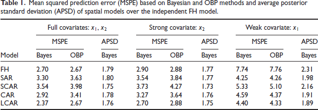
Mean squared prediction error (MSPE) based on Bayesian and OBP methods and average posterior standard deviation (APSD) of spatial models over the independent FH model.

Model	Full covariates: $x_1,x_2$			Strong covariate: $x_2$			Weak covariate: $x_{\mathrm{I}\mathrm{ }}$
	MSPE		APSD	MSPE		APSD	MSPE		APSD
	Bayes	OBP	Bayes	Bayes	OBP	Bayes	Bayes	OBP	Bayes
FH	2.70	2.67	1.79	2.90	2.88	1.77	7.74	7.76	2.31
SAR	3.30	3.63	1.80	3.54	3.84	I. 77	4.25	4.26	1.98
SCAR	3.54	3.98	1.75	3.73	4.27	1.73	5.33	5.10	2.16
CAR	2.92	3.41	1.78	3.27	3.64	1.76	4.59	4.37	1.91
LCAR	2.37	2.67	1.76	2.70	2.88	1.75	4.40	4.33	1.89

All the spatial models we consider here are described through the adjacency matrix of small areas $W=\left\{w_{ij}\right\},1\le i,j\le m$ , which plays an important role in capturing spatial association. Here, $w_{ij}=1$ if the $i$ th and $j$ th small areas are neighbors, and $w_{ij}=0$ , otherwise. Also, $w_{ii}=0$ for $=$ $1,\dots ,m$ . Let $w_{i.}={\sum }_{j=1}^m{w}_{ij}$ be the sum of the $i$ th row of $W$ and $L=\text{diag}{\left\{w_{i.}\right\}}_{i=1}^m$ . Assume that all small areas have at least 1 neighboring area. This implies that $L$ is p.d. We define $\tilde{W}=L^{-1}W$ . We present a few key facts about the eigenvalues of $W$ and $\tilde{W}$ . First, $W$ is a symmetric matrix, all its eigenvalues are real. We denote the $i$ th largest eigenvalue of $W$ by ${\lambda }_i\left(W\right),i=1,\cdots ,m$ . Since $W$ is non-null and $0={\sum }_{i=1}^m{w}_{ii}={\sum }_{i=1}^m{\lambda }_i\left(W\right)$ , it follows that ${\lambda }_m\left(W\right)<0<{\lambda }_1\left(W\right)$ . Since $\tilde{W}$ is a row stochastic matrix, all of its eigenvalues are bounded above by 1, and at least one of them is 1, that is, ${\lambda }_1\left(\tilde{W}\right)=1$ . Since $\tilde{W}$ and $L^{-1/2}W{L}^{-1/2}$ have the same eigenvalues, and the second matrix is symmetric, the eigenvalues of $\tilde{W}$ are real. Finally, $\text{tr}\left(\tilde{W}\right)=0$ implies ${\lambda }_m\left(\tilde{W}\right)$ must be negative.

We will use $R$ to denote the matrix $L-W$ . Four important spatially dependent random effects models are represented by the following positive definite matrices:

$${\text{SAR :Ω}}_2(\rho )={\left(I_m-\rho \tilde{W}\right)}^{\top }\left(I_m-\rho \tilde{W}\right),\rho \in (-1,1),$$

(3.1)

$$\text{SCAR}:{\text{Ω}}_3(\rho )=I_m-\rho W,\rho \in \left({\lambda }_m{(W)}^{-1},{\lambda }_1{(W)}^{-1}\right)\text{,}$$

(3.2)

$${\text{CAR :Ω}}_4(\rho )=L-\rho W,\rho \in \left({\lambda }_m{(\tilde{W})}^{-1},{\lambda }_1{(\tilde{W})}^{-1}\right)\text{,}$$

(3.3)

$$\text{LCAR}:{\text{Ω}}_5(\rho )=\rho R+(1-\rho )I_m,\rho \in (0,1)\text{,}$$

(3.4)

where $\rho$ is the spatial parameter that controls the strength of spatial dependence. Even though we are using the same notation $\rho$ in all four models, meaning of this parameter changes from one model to another. For the $k$ th model, $\rho$ varies between $l_k$ and $u_k,k=2,3,4,5$ ; these bounds are given above by (3.1)-(3.4). Chung and Datta^[4] argued that all the precision matrices above are positive definite. Note that $R={\text{Ω}}_4\left(1\right)={\text{Ω}}_5\left(1\right)$ , and the matrix $A^{-1}R$ is the precision matrix of the intrinsic autoregressive (IAR) model, another popular spatial model. This matrix is singular since $R$ is a singular matrix $\left(\Leftarrow R1=0\right)$ .

The model (3.2) is a simple version of conditional autoregressive model (Rao and Molina^[18], Ch. 9.6.2) where diagonal entries of the precision matrix are all equal to one. This model is known as the simple conditional autoregressive (SCAR) model. The model (3.3) is the widely used conditional autoregressive (CAR) model. Diagonal entries of the precision matrix are $L_{ii}$ for the CAR model, and these entries are between 1 and $L_{ii}$ for the LCAR model. The conditional autoregressive models, SCAR, CAR, and LCAR, assume that ${\theta }_i$ depends only on neighboring small area means. In other words, ${\theta }_i$ is correlated with ${\theta }_j$ ’s, $j\ne i$ , only for the surrounding areas. On the contrary, the simultaneous autoregressive (SAR) model assumes that ${\theta }_i$ is dependent on all other ${\theta }_j$ concurrently, $j\ne i$ , but has stronger (weaker) correlations for neighboring (remote) areas. The independent $\text{FH}$ model can be viewed as a special case of the SAR, SCAR, or LCAR model with $\rho =0$ . In an analogy to the spatial models, the precision matrix of the independent FH model is $I_m$ . For convenience of notation, although this precision matrix is free from $\rho$ , we denote it by ${\text{Ω}}_1\left(\rho \right)$ . We note that for various models we considered here the matrices $A^{-1}{\text{Ω}}_k,k=1,\cdots ,5$ correspond to the precision matrix $P_M$ in the model (2.2).

A full Bayesian analysis for the spatial models above based on a class of improper priors for $\beta$ and $A$ was pursued by Chung and Datta^[4]. For the CAR model with ${\text{Ω}}_4\left(\rho \right)$ with $\rho =1$ , the intrinsic CAR model (which we refer to here also as the IAR model), a fully Bayesian analysis based on a proper inverse gamma prior for $A$ has been considered by Vogt^[22] and Vogt et al.^[23]. Even though the IAR model is a limiting case of the $\text{CAR}\left(\rho \right)$ model with $\rho =1$ , Chung and Datta^[4] did not pursue the IAR model, and the proof of the propriety of the posterior for the CAR model will not automatically extend to the ICAR (or IAR) model without appropriate modification.

The EBLUP approach to small area estimation for some spatial models has been considered by several authors. Singh et al.^[20] made a pioneering effort for the SAR model. Following the approach of Datta and Lahiri^[5], Singh et al.^[20] derived a second-order approximation to the MSE of the EBLUP and a second-order unbiased estimator the MSE. Petrucci and Salvati^[14], Pratesi and Salvati^[17] and Pratesi et al.^[16] used Singh et al.^[20] results to several useful applications.

4. A Quasi-Bayesian Alternative to the OBP

For the independent Fay-Herriot model Datta et al.^[6] developed an alternative Bayesian version of the OBP method of Jiang et al.^[11]. While they referred to this method as pseudo-Bayes, the term pseudo’ seems to have a pejorative meaning. Consequently, in this article we will replace pseudo’ by quasi’.

In a recent article Liu et al.^[13] obtained a suitably justified estimator of the MSE of the OBP predictors of small area means for the independent Fay-Herriot model. However, derivation of the estimator is challenging and the estimator is occasionally negative. Quasi-Bayesian method of Datta et al.^[6] not only produces point estimates comparable with the OBPs, the associated posterior variances, naturally positive, are comparable with MSE estimates. Additionally, the quasiBayesian method provides useful credible intervals for the small area means in a straightforward manner. Even though the frequentist OBP point predictors for the spatial models can be calculated, no valid estimators of their MSEs are available yet. Any reasonable extension of the tedious calculations for the estimators of MSE, presented in Liu et al.^[13] only for the independent model, will be far more challenging for the spatial models. Moreover, these estimators may be negative. Due to much usefulness of both the spatial models and the OBP method, a quasi-Bayesian extension of Datta et al.^[6] solution for the independent Fay-Herriot model to a spatial dependent setup can serve as a way to provide reasonable credible intervals as well as uncertainty estimates of the estimators for small area means.

The standard Bayesian method updates a prior distribution of the parameters in a model by their likelihood. In a recent article, Bissiri et al.^[2] presented a general method to update a prior distribution for parameters to a posterior distribution when the parameters are connected to observations through a loss function rather than the traditional likelihood. Since the OBP procedure uses only a loss function and not the likelihood for the model parameters to estimate them, in our Bayesian analog to the OBP solution we use the OBP loss function and an algorithm from Bissiri et al.^[2] to create a quasi-likelihood function. Indeed, Datta et al.^[6] followed this algorithm to construct a quasi-likelihood from the OBP loss function under the independent Fay-Herriot model and a quasi-Bayesian solution from this likelihood.

4.1. Update of a Prior by a Loss Function: a Quasi-posterior

The discussion in this subsection is based on modification of Section 2.1 of Datta et al.^[6]. To derive a quasi-posterior pdf for $\psi$ , we adopt the framework for general Bayesian inference put forward by Bissiri et al.^[2]. According to these authors, the information’ about the parameter $\beta$ in the loss function $Q_0\left(\beta ,A,\rho ,y\right)$ should be appropriately calibrated to update the prior distribution for $\beta$ . We update the uniform prior on $\beta$ by creating an ad hoc likelihood’ for $\beta$ from this loss function. Since the loss function depends on the scale of the data $y$ , the ad hoc likelihood needs to be calibrated so that both the ad hoc likelihood and the prior pdf of $\beta$ become scale-free’.

In general, for some data $d$ with the density $f\left(d\mid \varphi \right)$ and prior $\text{pdf}\pi \left(\varphi \right)$ for the parameter $\varphi$ , the usual Bayes' rule updates the prior $\text{pdf}\pi \left(\cdot \right)$ to the posterior pdf determined by normalization of the kernel $f\left(d\mid \varphi \right)\pi \left(\varphi \right)$ of $\varphi$ . This kernel is proportional to $\text{exp}\left[-ws\left(\varphi ,d\right)-\text{log}\left(\pi \left({\varphi }^{\text{*}}\right)/\pi \left(\varphi \right)\right)\right]$ , where $s\left(\varphi ,d\right)=-\text{log}\left(f\left(d\mid \varphi \right)\right),w=1$ and ${\varphi }^{\text{*}}$ is a suitably chosen value of $\varphi$ . Bissiri et al.^[2] and Bissiri and Walker^[3] developed a general Bayesian method which generalizes the usual Bayes' rule to facilitate updating a prior pdf by loss information on the parameter $\varphi$ . A brief review of their solution is below.

If a nonnegative function $l\left(\varphi ,d\right)$ is the loss information on $\varphi$ based on data $d$ , Bissiri et al.^[2] suggests a general Bayes’ method to update a prior pdf $\pi \left(\varphi \right)$ by the normalized version of the kernel $\text{exp}\left[-w_{l}l\left(\varphi ,d\right)-\text{log}\left(\pi \left({\varphi }^{\text{*}}\right)/\pi \left(\varphi \right)\right)\right]$ , where $w_l>0$ is an appropriate constant to calibrate the loss information so that the components $w_{l}l\left(\varphi ,d\right)$ and $-\text{log}\left(\pi \left(\varphi \right)\right)$ are on a comparable scale. When $l\left(\varphi ,d\right)$ is $s\left(\varphi ,d\right)$ , the self-information loss, $w_l=1$ is the natural choice to combine the data loss with the prior $\text{loss}-\text{log}\left(\pi \left(\varphi \right)\right)$ to update the prior distribution. In our application, the loss function $Q_0\left(\beta ,A,\rho ,y\right)$ for $\beta$ is not a self-information loss. Bissiri et al.^[2] (cf. Section 3) argues that when different types of loss functions are combined, their calibration is crucial. In particular, the loss function should be commensurate to the prior distribution.

One way to combine two losses $l\left(\varphi ,d\right)$ and $-\text{log}\left(\pi \left(\varphi \right)\right)$ is based on a prior evaluation of the expected value of $l\left(\varphi ,d\right)$ to determine $w_l$ for the calibration (Bissiri et al.^[2], Section 3.2). To pick $w_l$ , solve

$$w_{l}E\left[l\left(\varphi ,d\right)\right]=E_{\pi }\left[\text{log}\left(\pi \left(\check{\varphi }\right)/\pi \left(\varphi \right)\right)\right],$$

(4.1)

where the left hand expectation $E\left[\cdot \right]$ is with respect to a joint distribution for $d$ and $\varphi$ , say $m\left(d,\varphi \right)$ , and the resulting marginal for $\varphi$ is $\pi \left(\varphi \right)$ . Here, $\check{\varphi }$ is taken as the maximizer of $\pi \left(\varphi \right)$ . Specifically, if $d$ given $\varphi$ has mean and variance $\varphi$ and ${\sigma }^2$ , respectively, and if $\pi \left(\varphi \right)$ is normal with mean $\eta$ and variance ${\tau }^2$ , then for squared error $\text{loss}l\left(\varphi ,d\right)={(\varphi -d)}^2$ , the scale $w_l$ is $1/\left(2{\sigma }^2\right)$ . This calibration relates the loss $w_{l}l\left(\varphi ,d\right)$ to the self-information loss for normally distributed data. The scaling constant $w_l$ is independent of both $\eta$ and ${\tau }^2$ . Hence, by taking a very large ${\tau }^2$ , one can approach a uniform prior for $\varphi$ and calibrate the squared error loss function relative to this approximate prior.

4.2. Calibration for $\beta$ : Quasi-posterior of $\beta$ Given $A,\rho$

We calibrate $Q_0\left(\beta ,A,\rho ,Y\right)$ , the first component of our loss function. For given $A,\rho$ , following an argument similar to the one from Section 2.2 of Datta et al.^[6], we find that for a multivariate normal

prior for $\beta$ an appropriate scaling factor, $w_0$ , is given by

$$w_0=\frac{m}{2}{[\text{tr}\left\{BD\right\}]}^{-1}.$$

The matrix $B$ has been defined following equation (2.3). This scalar $w_0$ is free from the parameters of the multivariate normal prior. By taking the variance of this prior very large’, we can use the traditional uniform prior for $\beta$ . Thus the posterior for $\beta$ is

$${\pi }_{qs}\left(\beta \mid A,\rho ,y\right)\propto \text{exp}\left[-w_0{Q}_0\left(\beta ,A,\rho ,y\right)\right],$$

(4.2)

see (Bissiri et al.^[2]). The above posterior distribution, conditional on $A,\rho$ , is multivariate normal with mean vector ${\tilde{\beta }}_O\left(\delta \right)={\left(X^T{B}^{T}BX\right)}^{-1}{X}^T{B}^{T}BY$ and variance-covariance matrix ${\left(2w_0{X}^T{B}^{T}BX\right)}^{-1}$ .

4.3. Approximate Calibration of Loss Function for $A$ and $\rho$

The two-step minimization of the loss function $Q\left(\beta ,A,\rho ,y\right)$ to estimate the model parameters gives the loss function $Q_{\text{*}}\left(A,\rho \right)=Q\left(\tilde{\beta }\left(A,\rho \right),A,\rho ,Y\right)$ for $A$ and $\rho$ . For a prior $\pi \left(A,\rho \right)$ on $A$ and $\rho$ , we need to calibrate the loss function $Q_{\text{*}}\left(A,\rho \right)$ by suitable weight $w_{\text{*}}$ to create a quasi-likelihood for $A$ and $\rho$ .

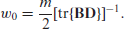
Let $\overline{D}={\sum }_{i=1}^m{D}_i/m$ . We use a uniform prior for $\rho$ over its allowable range $\left(l_k,u_k\right)$ , and an independent prior ${\pi }_A\left(A\right)=\stackrel{࿽}{D}{(A+\stackrel{࿽}{D})}^{-2}$ . It can be shown that ${\int }_0^{\infty }{\int }_{l_k}^{u_k}\text{log}\left[{\pi }_A\left(\check{A}\right)/{\pi }_A\left(A\right)\right]{\pi }_A\left(A\right){\pi }_{\rho }\left(\rho \right)d\rho dA=2$ . We remark that this value is specific to the prior ${\pi }_A\left(A\right)$ . For another proper prior ${\pi }_A^{\text{*}}\left(A\right)$ , we need to recompute the corresponding value, which we may do by the Monte Carlo method. We also need to compute $E\left[Q_{\text{*}}\left(A,\rho \right)/m\right]$ , where the expectation is with respect to the joint distribution of $Y$ and the model parameters. We can simplify this via iterative expectation by using the first two moments of $Y$ (given $,A,\rho$ ). The result depends on $A,\rho$ , but not on $\beta$ , and we find the Monte Carlo expectation of this function with respect to the prior for $A$ and $\rho$ by drawing 10000 values for the pair from their joint prior distribution. Using this value, we get the calibration coefficient $w_{\text{*}}$ using appropriate modification of the equation (4.1).

Using the above calibration weight, for the loss function $Q_{\text{*}}\left(A,\rho \right)$ , an update of the prior $\pi \left(A,\rho \right)$ is given by the quasi-posterior

$${\pi }_{qs}\left(A,\rho \mid y\right)\propto {(A+\stackrel{࿽}{D})}^{-2}\text{exp}\left[-w_{\text{*}}{Q}_{\text{*}}\left(A,\rho \right)\right]I\left(l_k<\rho <u_k\right).$$

(4.3)

To make quasi-Bayesian inference on $\theta$ , first generate generate $A$ and $\rho$ from the quasi-posterior in (4.3), then use the generated $A$ and $\rho$ to get $\beta$ from its conditional quasi-posterior in (4.2). Finally, use the generated values of $\beta ,A,\rho$ to draw $\theta$ from an MVN distribution with mean ${\tilde{\theta }}_B\left(\psi \right)$ in (2.3) and variance-covariance matrix ${\left(P_D+P_M\right)}^{-1}$ .

For a suitably large $S$ , we generate ${\theta }^{\left(s\right)},s=1,\cdots ,S$ , following the method outlined above. Based on these generated values of ${\theta }^{\left(s\right)}$ , we can create various summaries of the posterior distribution including the posterior mean, variance and posterior quantiles of ${\theta }_i,i=1,\cdots ,m$ to find their point estimates and credible intervals.

Finally, for the IAR model we have no spatial correlation parameter $\rho$ and the precision matrix of $v$ is given by $A^{-1}R$ . Using this precision matrix we can easily obtain $Q_0\left(\beta ,A,Y\right)$ and $Q_1\left(A\right)$ , which will provide the quasi-posterior distributions of $\beta$ and $A$ .

5. Application to the Current Population Survey Data

We apply our quasi-Bayesian method for the spatial models to estimate the four-person family median incomes for forty-eight states of the continental US and the District of Columbia for the income year 1989. We exclude Alaska and Hawaii from this application because they are geographically isolated from the continental US. The US Department of Health and Human Services (HHS) needs accurate state-level median income estimates to implement an energy assistance program for low-income families. The yearly household income data is collected from the Annual Demographic Supplement to the monthly Current Population Survey (CPS). The state-level estimates for most states from the CPS sample, unfortunately, are not adequately accurate. Using the CPS estimates as direct estimates, and relevant administrative data and past census data as covariates, the US Census Bureau developed model based estimates of the median incomes by using the regular Fay-Herriot model with independent random effects. In this application, we develop alternative small area estimates of median incomes based on the spatial models and compare their performances with the estimates from the traditional Fay-Herriot model. We consider estimation of incomes for the year 1989 since more accurate estimates of the 1989 unknown incomes are available from the 1990 decennial census. Since census values are accurate, we treat these estimates as true values’ and compare our various predictions against these values.

We denote the true 1989 four-person family median income for $i$ th state by ${\theta }_i$ , and the direct estimate of ${\theta }_i$ from the 1990 CPS by $Y_i$ . Two available covariates for this problem are

$x_{i1}$ : 1979 four-person family median income of the ith state from the 1980 census,

$x_{i2}=\left(PC{I}_{i,1989}/PC{I}_{i,1979}\right)\cdot x_{i1}$ : adjusted 1979 census four-person family median income of the ith state,

where PCI is state level per capita income from the U.S. Bureau of Economic Analysis. From our present and previous analyses (cf. Chung and Datta^[4] and Datta et al.^[6]) we found that the covariate $x_2$ is more effective in accounting the variability of the median income in small areas. When we look at the spatial dependence within each covariate, we find that the Moran’s I measuring the spatial dependence for the 1989 census state median incomes is 0.50. The corresponding value for $x_2$ is 0.43. The Moran’s I for the direct estimates $y_i$ from the 1989 CPS is 0.31. But the same for $x_1$ is 0.22. While the CPS estimates track closely in terms of Moran’s I of the true’ values, the 1989 census values, they have high variances. Based on Moran’s I, borrowing information from $x_2$ may be more effective than using $x_1$ to track spatial patterns of ${\theta }_i$ ’s. We use mean squared prediction error (MSPE) from the truth’ ${\theta }_i$ , which are unknown. In their place, we use the median income values we obtained from the 1990 census. We denote these values by $C_{i,89}$ . We also compute average of posterior standard deviations (APSD) to evaluate the accuracy of predictions. We define these criteria by

$$MSPE =\frac{1}{m_E}{\displaystyle \sum }_{i\in E}{\left({\hat{\theta }}_i-C_{i,89}\right)}^2,$$

(5.1)

$$APSD=\frac{1}{m_E}{\displaystyle \sum }_{i\in E}sd\left({\theta }_i\right),$$

(5.2)

where ${\hat{\theta }}_i$ is the estimated value from each model and ${\theta }_i$ is the true median income value. Here $E$ is a suitable subset of $\left\{1,\cdots ,m\right\}$ , which is determined by indices only of the sampled or non-sampled small areas, and $m_E$ is the number of elements in $E$ . Finally, $sd\left({\theta }_i\right)$ is the posterior standard deviation of ${\theta }_i$ based on the model under consideration.

5.1. Median Incomes of 4-person Families by State

We fit four spatial models defined by (3.1) to (3.4) and the FH model with three subsets of covariates, given by the design matrix $X=\left[1_m,x_1,x_2\right]$ , or $X=\left[1_m,x_2\right]$ , or $X=\left[1_m,x_1\right]$ . The first setting is the most efficient one and the last setting is the least efficient. We calculate the MSPEs and APSDs over 49 areas from respective ${\theta }_i$ ’s and results are summarized in Table 1. Results reported for Bayes are based on the quasi-Bayes predictors we develop here.

Table 1 above shows that for the most efficient set of covariates (full covariates) the LCAR model has about 12 per cent smaller MSPE and 2 per cent smaller APSD than those of the independent FH model for quasi-Bayes. Since $x_2$ displays a good spatial pattern, it can explain most of the variability of ${\theta }_i$ . As a result, it is not surprising that in terms of MSPE, except the LCAR model, the independent FH model is at least as good as the spatial models. In terms of the APSD values, all five models are comparable. Moreover, in terms of MSPE, quasi-Bayes outperforms OBP method for all four spatial models. The quasi-Bayes method has about 14 per cent smaller MSPE than those of the OBP method of CAR model.

On the other extreme, when only the weaker variable $x_1$ is included in the regression model, it is no surprise that the MSPE and the APSD for all five models are higher in comparison with the other two combinations of covariates for both quasi-Bayes and OBP. In this case, under quasi-Bayes method, however, the MSPE and the APSD of the SAR are approximately 45 per cent and 14 per cent, respectively, less than those of the independent FH model. The LCAR is the second-best model in terms of MSPE, with an MSPE that is 43 per cent smaller, and in terms of the APSD the LCAR is the best for which the APSD is 18 per cent smaller than that for the independent FH model. By removing the strong covariate $x_2$ from the full model, the MSPE of the SAR and LCAR models increase by about 29 per cent and 86 per cent, respectively, while the MSPE of the independent FH model increases by roughly 187 per cent. These results show that when covariates are less than effective in explaining existing spatial variation, spatial models that account for such variation can generate much more accurate predictions than the independent FH model.

Table 1 provides MSPE values for the OBP method. In terms of the MSPE, only when the weak covariate is used in the regression function, the OBP only marginally performs better than the quasiBayes predictors for the SCAR and CAR models. However, the OBP has no estimated root mean squared error of prediction for spatial models.

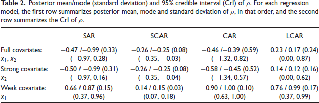
In Table 2 we provide point estimates and credible intervals of the spatial parameter for various models. Among the three sets of regression models we considered, only for the case of $x_1$ , credible intervals of the spatial parameter for all four models do not include 0, the null value; these intervals quite strongly indicate the presence of a significantly nonzero spatial pattern.

Table 2.

Posterior mean/mode (standard deviation) and 95% credible interval (Crl) of $\rho$ . For each regression model, the first row summarizes posterior mean, mode and standard deviation of $\rho$ , in that order, and the second row summarizes the Crl of $\rho$ .

	SAR	SCAR	CAR	LCAR
Full covariates:	$-0.47/-0.99\left(0.33\right)$	$-0.26/-0.25\left(0.08\right)$	$-0.46/-0.39\left(0.59\right)$	$0.23/0.17\left(0.24\right)$
$x_1,x_2$	$\left(-0.97,0.28\right)$	$\left(-0.35,-0.03\right)$	$\left(-1.32,0.82\right)$	$\left(0.00,0.87\right)$
Strong covariate:	$-0.50/-0.99\left(0.31\right)$	$-0.26/-0.25\left(0.08\right)$	$-0.58/-0.45\left(0.52\right)$	$0.14/0.12\left(0.16\right)$
$x_2$	$\left(-0.97,0.16\right)$	$\left(-0.35,-0.04\right)$	$\left(-1.34,0.57\right)$	$\left(0.00,0.62\right)$
Weak covariate:	$0.66/0.87\left(0.15\right)$	$0.14/0.15\left(0.03\right)$	$0.90/1.00\left(0.10\right)$	$0.76/0.99\left(0.17\right)$
$x_1$	$\left(0.37,0.96\right)$	$\left(0.07,0.18\right)$	$\left(0.63,1.00\right)$	$\left(0.37,0.99\right)$

5.2. Estimation of Some Non-sampled State Means

We evaluate the spatial models in terms of the accuracy of their predictions for non-sampled small areas. In this study we have evaluated both the approaches, quasi-Bayesian and OBP. Again, our two covariate settings are $X=\left[1,x_1\right]$ and $X=\left[1,x_2\right]$ . To check the quality of prediction for non-sampled areas with no direct estimates, we follow an idea of Chung and Datta^[4]. Suppose there are $m_1$ nonsampled areas and $m_2=m-m_1$ sampled areas. We constructed 12 data sets in an arbitrary manner, eleven of which lack four $\left(m_1=4\right)$ direct estimates and one lacks five $\left(m_1=5\right)$ direct estimates. We do not use CPS estimates (direct estimates) of the states omitted at each example and predict the ${\theta }_i$ ’s of the omitted states. Suppose ${\theta }_{\left(1\right)}$ is the subvector of $\theta$ corresponding to the non-sampled areas, and ${\theta }_{\left(2\right)}$ is the subvector of $\theta$ corresponding to the sampled areas. Let $Y_{\left(2\right)}$ denote the vector of direct estimates for the sampled areas. We arrange the elements of $\theta$ and define an indicator matrix $M$ so that ${\theta }_{\left(2\right)}=M\theta$ . The matrix $M$ is $m_2\times \left(m_1+m_2\right)$ with its last $m_2$ columns form an identity matrix, and the first $m_1$ columns are null vectors. We then define $X_{\left(2\right)}=MX$ .

We obtain OBP and quasi-Bayes predictions of ${\theta }_{\left(1\right)}$ based on $Y_{\left(2\right)}$ for all five models. Using these predictions, we compute, for each non-sampled area under the FH model and spatial models for each data set, the squared prediction error for both the quasi-Bayes and OBP point predictors. Obviously, we get the posterior standard deviations only for the quasi-Bayes method. We summarize the mean squared prediction error (MSPE) over non-sampled areas for each data set in Table 4 and average posterior standard deviation (APSD) in Table 3. Evaluation of prediction performance is based on the following ratios:

$$MSPE\_Rati{o}_{ki}=\frac{msp{e}_{ki}}{msp{e}_{1i}},APSD\_Rati{o}_{ki}=\frac{aps{d}_{ki}}{aps{d}_{1i}},i=1,\cdots ,12;k=2,\cdots ,5$$

Table 3.

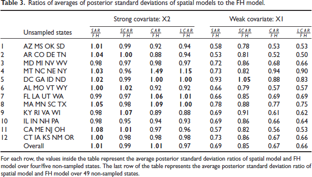
Ratios of averages of posterior standard deviations of spatial models to the $\mathrm{F}\mathrm{H}$ model.

	Unsampled states	Strong covariate: X2				Weak covariate: XI
		$\frac{SAR}{FH}$	$\frac{SCAR}{FH}$	$\frac{CAR}{FH}$	$\frac{LCAR}{FH}$	$\frac{SAR}{FH}$	$\frac{SCAR}{FH}$	$\frac{CAR}{FH}$	$\frac{LCAR}{FH}$
I	AZ MS OK SD	1.01	0.99	0.92	0.94	0.58	0.78	0.53	0.53
2	AR CO DE TN	1.04	1.00	0.88	0.94	0.53	0.81	0.52	0.50
3	MD MI NV WV	0.98	0.97	0.98	0.97	0.72	0.86	0.68	0.66
4	MT NC NE NY	1.03	0.96	1.49	1.15	0.73	0.82	0.94	0.90
5	DC GA ID ND	1.02	0.99	1.00	1.00	0.93	1.05	0.88	0.83
6	AL MO VT WY	1.00	1.02	0.92	0.92	0.66	0.79	0.57	0.57
7	FL LA UT WA	0.99	0.97	1.06	1.01	0.66	0.85	0.69	0.69
8	MA MN SC TX	1.05	0.98	1.09	1.00	0.78	0.88	0.77	0.75
9	KY RI VA WI	0.98	1.07	0.89	0.88	0.69	0.91	0.61	0.62
10	IL IN NH PA	0.98	0.95	0.94	0.93	0.69	0.86	0.66	0.64
II	CA ME NJ OH	1.08	1.01	0.97	0.96	0.57	0.82	0.56	0.53
12	CT IA KS NM OR	1.00	0.98	0.98	0.98	0.73	0.86	0.67	0.66
	Overall	1.01	0.99	1.01	0.97	0.69	0.85	0.67	0.66

For each row, the values inside the table represent the average posterior standard deviation ratios of spatial model and $\mathrm{F}\mathrm{H}$ model over four/five non-sampled states. The last row of the table represents the average posterior standard deviation ratio of spatial model and FH model over 49 non-sampled states.

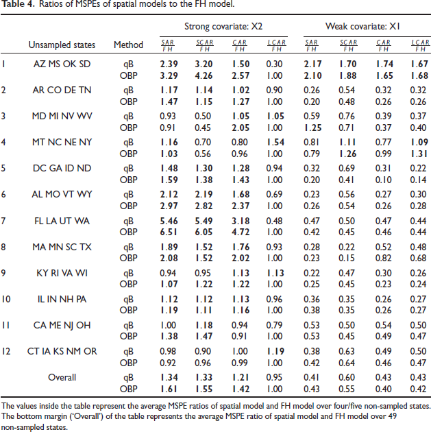
where $aps{d}_{ki}$ is the average posterior standard deviations of all omitted $\theta$ ’s (four or five) under the $k$ th model for the $i$ th data set. A similar meaning is for $msp{e}_{ki}$ . The value of MSPE_Ratio ${ }_{ki}$ or APSD_Ratio k ${ }_{\text{i }}$ less than one means that the kth spatial model using ith data set has a smaller mean squared prediction error or average posterior standard deviation than the FH model. Ratios higher than one are highlighted in bold in Table 3 and Table 4.

Table 4.

Ratios of MSPEs of spatial models to the FH model.

	Unsampled states	Method	Strong covariate: $\mathrm{X}2$				Weak covariate: $\mathrm{X}\mathrm{I}$
			$\frac{SAR}{FH}$	$\frac{SCAR}{FH}$	$\frac{CAR}{FH}$	$\frac{LCAR}{FH}$	$\frac{SAR}{FH}$	$\frac{SCAR}{FH}$	$\frac{CAR}{FH}$	$\frac{LCAR}{FH}$
1	AZ MS OK SD	qB	2.39	3.20	1.50	0.30	2.17	1.70	1.74	1.67
		OBP	3.29	4.26	2.57	1.00	2.10	1.88	1.65	1.68
2	AR CO DE TN	qB	1.17	1.14	1.02	0.90	0.26	0.54	0.32	0.32
		OBP	1.47	1.15	1.27	1.00	0.20	0.48	0.26	0.26
3	MD MI NV WV	qB	0.93	0.50	1.05	1.05	0.59	0.76	0.39	0.37
		OBP	0.91	0.45	2.05	1.00	1.25	0.71	0.37	0.40
4	MT NC NE NY	qB	1.16	0.70	0.80	1.54	0.81	1.11	0.77	1.09
		OBP	1.03	0.56	0.96	1.00	0.79	1.26	0.99	1.31
5	DC GA ID ND	qB	1.48	1.30	1.28	0.94	0.32	0.69	0.31	0.22
		OBP	1.59	1.38	1.43	1.00	0.20	0.41	0.10	0.14
6	AL MO VT WY	qB	2.12	2.19	1.68	0.69	0.23	0.56	0.27	0.30
		OBP	2.97	2.82	2.37	1.00	0.26	0.54	0.26	0.28
7	FL LA UT WA	qB	5.46	5.49	3.18	0.48	0.47	0.50	0.47	0.44
		OBP	6.51	6.05	4.72	1.00	0.42	0.45	0.46	0.44
8	MA MN SC TX	qB	1.89	1.52	1.76	0.93	0.28	0.22	0.52	0.48
		OBP	2.08	1.52	2.02	1.00	0.23	0.15	0.82	0.68
9	KY RI VA WI	qB	0.94	0.95	1.13	1.13	0.22	0.47	0.30	0.26
		OBP	1.07	1.22	1.22	1.00	0.25	0.45	0.23	0.24
10	IL IN NH PA	qB	1.12	1.12	1.13	0.96	0.36	0.35	0.26	0.27
		OBP	1.19	1.11	1.16	1.00	0.38	0.35	0.26	0.27
11	CA ME NJ OH	qB	1.00	1.18	0.94	0.79	0.53	0.50	0.54	0.50
		OBP	1.38	1.47	0.91	1.00	0.53	0.45	0.49	0.47
12	CT IA KS NM OR	qB	0.98	0.90	1.00	1.19	0.38	0.63	0.49	0.50
		OBP	0.92	0.96	0.99	1.00	0.42	0.64	0.46	0.47
	Overall	qB	1.34	1.33	1.21	0.95	0.41	0.60	0.43	0.43
		OBP	1.61	1.55	1.42	1.00	0.43	0.55	0.40	0.42

The values inside the table represent the average MSPE ratios of spatial model and FH model over four/five non-sampled states. The bottom margin ('Overall') of the table represents the average MSPE ratio of spatial model and FH model over 49 non-sampled states.

When using a weak covariate, the MSPEs and APSDs of SAR, SCAR, CAR, and LCAR models for the non-sampled states are usually smaller than those based on the independent FH model. Their Overall’ MSPE ratios (to the FH independent model) are $0.41,0.60,0.43$ and 0.43, respectively. The Overall’ APSD ratios are $0.69,0.85,0.67$ and 0.66, respectively. Both SAR and CAR models produce an MSPE ratio greater than 1 for one data set, whereas SCAR and LCAR models produce MSPE ratios greater than 1 for two data sets. Even after substantial exploratory analysis we have been unable to hit on a possible explanation for this anomaly.

For the more effective covariate setting, in terms of both MSPE and APSD ratios, except the LCAR model all other spatial models fare worse than the independent FH model. In this case, the LCAR model has the smallest MSPE ratio of 0.95 and the APSD ratio of 0.97.

Table 5.

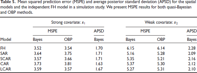
Mean squared prediction error (MSPE) and average posterior standard deviation (APSD) for the spatial models and the independent FH model in a simulation study. We present MSPE results for both quasi-Bayesian and OBP methods.

Model	Strong covariate: $x_I$			Weak covariate: $x_2$
	MSPE		APSD	MSPE		APSD
	Bayes	OBP	Bayes	Bayes	OBP	Bayes
$\text{FH}$	3.52	3.54	1.70	6.15	6.14	2.28
SAR	3.64	3.75	I.7I	5.16	5.28	2.09
SCAR	3.57	3.66	I.7I	5.35	5.21	2.16
CAR	3.73	3.81	1.63	5.37	5.30	2.12
LCAR	3.59	3.57	I. 67	5.27	5.31	2.10

Finally, from the right half of Table 4 we see that for the weak covariate case, the average MSPEs for the OBP predictors are lower under the spatial models than under the independent FH model. Also, the same part of this table shows that improvements in these MSPE ratios are slightly better for the OBP method than for the quasi-Bayesian method. However, for the SAR model, the Bayesian method is at least as good as the OBP method. We reiterate that while the Bayesian method provides a measure of uncertainty of the point estimates, the OBP method has no such measure available.

6. Simulation Studies

In this section, we present two simulation studies to examine our proposed quasi-Bayes approach to spatial models under two scenarios. To make the simulation setting realistic, we mimic the 1989 4 -person family median income data described in Section 5. The first scenario evaluates the quality of prediction under two different informative covariate settings with all contiguous $\text{m}=49$ areas (48 states and Washington, D.C.) of U.S. and the second scenario evaluates the quality of prediction in the absence of direct estimates, details are shown in Subsections 6.1 and 6.2, respectively.

6.1. A Simulation Study Without Non-sampled Areas

In the first simulation, we mainly evaluate the quality of prediction under different covariate settings, strong and weak covariates. There are no non-sampled areas. For each setting, we consider S $=100$ replicated data sets.

Data generation: We use the $D_i$ values from the application as the $D_i$ ’s in the simulations. Let $\stackrel{࿽}{D}=$ $m^{-1}{\sum }_{i=1}^m{D}_i$ . We set $\rho =0.85$ so that the Morans I values of 100 replicated small area means range from 0.32 to 0.66 with mean 0.50 (which is consisitent with Moran’s I value for the 1989 census state median incomes in Section 5) and $A=\stackrel{࿽}{D}/2$ and consider two independent covariates $x_1$ and $x_2$ with SAR spatial dependence, that is, $x_1,x_2\sim N_m\left(0_m,{\left\{{\Omega }_2\left(\rho \right)\right\}}^{-1}\right)$ . Then, letting ${\left({\beta }_1,{\beta }_2\right)}^{\top }={(2,1)}^{\top }$ and $\mu ={\beta }_1{x}_1+{\beta }_2{x}_2$ , we generate small area means and direct estimates from the following independent FH model:

$$\theta \sim N_m\left(\mu ,A{I}_m\right),Y\mid \theta \sim N_m\left(\theta ,D\right).$$

The covariate $x_1\left(x_2\right)$ introduces stronger (weaker) spatial pattern to the ${\theta }_i$ ’s, and we refer $x_1\left(x_2\right)$ as the strong (weak) covariate.

The simulation outcomes presented in Table 5 align with the real data analysis outcomes presented in Table 1. At the strong covariate setting, the independent model is a very competitive model for both quasi-Bayes and OBP methods. At the weak covariate setting, the LCAR model has roughly 14 per cent smaller MSPE (quasi-Bayes method) and 8 per cent lower APSD than the FH model. In contrast, with the strong covariate setting, the MSPE and APSD values for the LCAR and FH models are comparable since $x_2$ can explain the majority of variability of ${\theta }_i$ ’s. Moreover, when only the weaker variable $x_1$ is included in the regression model, the MSPE and APSD for all five models are greater than their counterparts when only the stronger covariate $x_2$ is included. Across these covaiate settings, the MSPEs of the SAR, SCAR, CAR and LCAR models increase by approximately 42 per cent, 50 per cent, 44 per cent and 47 per cent, respectively, for the quasi-Bayes method, and 41 per cent, 42 per cent, 39 per cent and 49 per cent, respectively, for the OBP method. While the MSPE of the independent FH model increases by 75 per cent and 73 per cent, respectively for the quasi-Bayes and OBP methods. These results again validate usefulness of spatial models when available covariates are not much effective in explaining existing spatial variation.

6.2. A Simulation Study with Non-sampled Areas

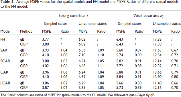
In the second simulation study, we compare prediction performances of the $\text{FH}$ model and the four spatial models in the absence of informative covariates with several non-sampled areas. Following the setup in Chung and Datta^[4], we also do not simulate direct estimates for the following $m_1=7$ states: Delaware, Massachusetts, Michigan, Nebraska, Rhode Island, South Dakota, and Texas. For the remaining $m_2=42$ areas we have direct estimates.

Data generation: Similar to the first simulation, the only difference is we do not simulate direct estimates of $m_1=7$ states. We denote $\overline{D}=m_2^{-1}{\sum }_{i=1}^{m_2}{D}_i$ and $D_{\left(2\right)}=\text{diag}{\left\{D_i\right\}}_{i=1}^{m_2}$ . We set $\rho =0.85$ and $A=\stackrel{࿽}{D}/2$ and consider two independent covariates $x_1$ and $x_2$ with SAR spatial dependence, that is, $x_1,x_2\sim N_m\left(0_m,{\left\{{\Omega }_2\left(\rho \right)\right\}}^{-1}\right)$ . Then, letting ${\left({\beta }_1,{\beta }_2\right)}^{\top }={(2,1)}^{\top }$ and $\mu ={\beta }_1{x}_1+{\beta }_2{x}_2$ . However, we generate small area means and direct estimates from the following independent FH model:

$$\theta \sim N_m\left(\mu ,A{I}_m\right),Y_{\left(2\right)}\mid {\theta }_{\left(2\right)}\sim N_m\left({\theta }_{\left(2\right)},D_{\left(2\right)}\right),$$

where the components of $Y_{\left(2\right)}$ and ${\theta }_{\left(2\right)}$ correspond to the $m_2$ sampled small areas.

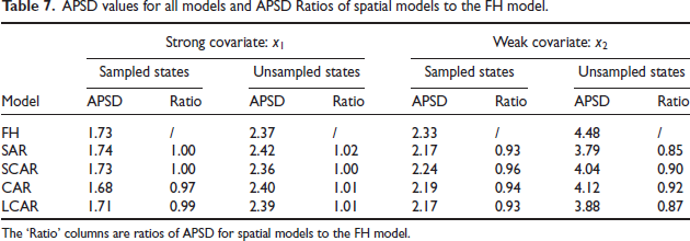
Table 6 presents the average MSPE and MSPE ratios across four spatial models and the FH model if only the strong or weak covariate $x_2$ or $x_1$ is included. When only a strong covariate is given, the independent model is a very competitive model for both quasi-Bayes and OBP methods for both sample states and non-sampled states. Improvements are greater when only a weak covariate is added compared to when only a strong covariate is included. For the quasi-Bayes method under weak covariate setting, LCAR and SAR models have roughly 12 per cent and 13 per cent lower MSPEs than the FH model for sampled states, respectively. For un-sampled states, both LCAR and SAR models have about 33 per cent lower MSPEs than the FH model. We reach a similar conclusion about the spatial models when we compare them in terms of APSD presented in Table 7. Overall, among the four spatial models, LCAR is the most competitive, considering the data were generated using the SAR model. In terms of MSPEs our quasi-Bayes predictors generally outperform the OBP predictors for all spatial models.

Table 6.

Average MSPE values for the spatial models and FH model and MSPE Ratios of different spatial models to the $\text{FH}$ model.

Model	Method	Strong covariate: $x_1$				Weak covariate: $x_2$
		Sampled states		Unsampled states		Sampled states		Unsampled states
		MSPE	Ratio	MSPE	Ratio	MSPE	Ratio	MSPE	Ratio
$\text{FH}$	$qB$	3.77	I	6.02	I	6.43	I	17.38	I
	OBP	3.80	I	6.02	I	6.43	I	17.38	I
SAR	$qB$	3.93	1.04	6.56	1.09	5.60	0.87	11.63	0.67
	OBP	4.10	1.08	7.10	1.18	5.74	0.89	12.54	0.72
SCAR	$qB$	3.88	1.03	6.31	1.05	5.82	0.91	12.14	0.70
	OBP	4.02	1.06	6.68	I.II	5.72	0.89	12.32	$0.7\text{I}$
CAR	$qB$	3.96	1.06	6.24	1.04	5.88	0.91	13.66	0.79
	OBP	4.10	1.08	6.59	1.09	5.84	0.91	13.90	0.80
LCAR	$qB$	3.86	1.02	6.29	1.04	5.66	0.88	11.40	0.66
	OBP	3.87	1.02	6.35	1.05	5.73	0.89	12.16	0.70

The Ratio’ columns are ratios of MSPE for spatial models to the FH model. We abbreviate quasi-Bayes by qB.

Table 7.

APSD values for all models and APSD Ratios of spatial models to the FH model.

Model	Strong covariate: $x_1$				Weak covariate: $x_2$
	Sampled states		Unsampled states		Sampled states		Unsampled states
	APSD	Ratio	APSD	Ratio	APSD	Ratio	APSD	Ratio
$\text{FH}$	1.73	I	2.37	I	2.33	I	4.48	I
SAR	I. 74	1.00	2.42	1.02	2.17	0.93	3.79	0.85
SCAR	1.73	1.00	2.36	1.00	2.24	0.96	4.04	0.90
CAR	1.68	0.97	2.40	1.01	2.19	0.94	4.12	0.92
LCAR	I.71	0.99	2.39	1.01	2.17	0.93	3.88	0.87

The Ratio’ columns are ratios of APSD for spatial models to the FH model.

7. Conclusions

Jiang et al.^[11] suggested the OBP method as an alternative to the EBLUP method to predict small area means. Although these authors suggested the OBP approach for a general mixed effects model, accurate estimation of the mean squared error of the OBP predictors of small area means are available only for the independent Fay-Herriot model (cf. Liu et al.^[13]). Derivation of the MSE estimator by Liu et al.^[13] is tedious and the estimator is not guaranteed to be positive. No such results are available for spatial random effects models. Spatial random effects models provide useful prediction of small area means in the absence of good covariates to explain the spatial variation of the small area means (cf. Chung and Datta^[4]). In this work, we have developed a quasi-Bayesian version of the OBP method for prediction of small area means based on various spatial random effects model. This work is a generalization for spatial models of the quasi-Bayesian method by Datta et al.^[6]. It also generalizes the regular Bayesian spatial method of Chung and Datta^[4] for the OBP method based on a quasi-Bayesian argument. Evaluation of the proposed quasi-Bayes spatial predictions based on available Census data and realistic simulations show the usefulness of quasi-Bayesian spatial predictors of small area means. These methods are straightforward to implement to create reliable measures of uncertainty and credible intervals for the small area means.