
Abstract
This article offers a non-technical review of selected applications that combine survey and geospatial data to generate small area estimates of wealth or poverty. Publicly available data from satellites and phones predict poverty and wealth accurately across space, when evaluated against census data, and their use in model-based estimates improves the accuracy and efficiency of direct survey estimates. Models based on interpretable features appear to predict more accurately than estimates derived from convolutional neural networks. Estimates for sampled areas are significantly more accurate than those for non-sampled areas due to informative sampling. In general, estimates benefit from using geospatial data at the most disaggregated level possible. Tree-based machine learning methods appear to generate more accurate estimates than linear mixed models in common settings. Small area estimates using geospatial data can improve the design of social assistance programmes, particularly when the existing targeting system is poorly designed.
Introduction
Using geospatial data as auxiliary data for small area estimation is an old idea. Proof of concept was initially demonstrated 35 years ago by Battese et al.,[1] who combined survey data with early imagery from the Landsat satellite to predict the area under Corn and Soybean production in 11 counties in Iowa. That paper is widely cited in the field of small area estimation statistics, with nearly 1,100 cites on Google Scholar as of May 2023. But the paper is better known for another seminal contribution, as it was the first to develop and apply the well-known nested-error unit-level model, with a conditional random effect specified at the target area level, to estimate means for small areas. From 1988 to about 2015, economists and statisticians devoted considerable effort to refining this model in various ways, with a particularly important innovation introduced by Molina and Rao,[2] to estimate indicators other than means, such as poverty headcount rates, using simulation techniques. In the meantime, the publication of Elbers et al.[3] (ELL), which used a slightly different unit-level model, popularized the use of small area estimation at the World Bank. Nonetheless, until relatively recently, virtually all applications during this time used census or other administrative data as auxiliary data, ignoring geospatial data as a potential source of auxiliary data from which surveys could borrow strength’ to improve the measurement of socio-economic data.
Geospatial data were rediscovered as a potential source of auxiliary data in the mid 2010s, as advances in computing power and storage enabled geospatial data to become publicly available at a wide scale, as surveys began to be regularly implemented on tablets that collect geocoordinates and as a new generation of data scientists, economists and statisticians discovered the potential of geospatial data to improve socio-economic measurement. This, in turn, sparked interest in combining survey and satellite indicators for the purposes of small area estimation. Using appropriate methods for this type of data fusion’ is important because small area poverty estimates have implications for targeting and evaluating public interventions and can shed light on economic geography more generally. At the same time, in part because of recent advances in machine learning algorithms, different disciplines and authors have taken very different methodological approaches to combining geospatial data and survey data for the purposes of small area estimation.
This article provides a non-technical review of selected evidence from this relatively new literature. It builds on two recent reviews[4, 5] but focuses exclusively on the small area estimation of wealth and poverty, devoting particular attention to differences in statistical methodology across studies. In particular, we ignore some of the excellent recent work on agricultural crops and yields,[6, 7] labour[8] and other indicators. There is now a robust literature documenting that estimates of wealth and poverty derived from survey and geospatial data are correlated with benchmarks derived from surveys or censuses. The strength of these correlations varies widely and depends on a myriad number of factors, including the country context, the method used for prediction, the target area for prediction, the exact indicator being predicted, the choice of geospatial variables and the nature of the training and evaluation data.
Because the literature is relatively new, no consensus has yet emerged around the optimal prediction method in different contexts. Furthermore, comparisons of alternative prediction methods in the same geographic context remain rare, and some of the few examples of these comparisons have not yet been published in peer reviewed journals. Therefore, most of the evidence presented below on comparisons across alternative models should be interpreted as tentative priors based on limited evidence from specific contexts.
This review is divided into three sections. The first section begins by very briefly describing some of the many publicly available geospatial indicators. It then reviews selected studies from a rapidly growing literature evaluating the accuracy of small area estimates of wealth and poverty using geospatial data, documenting strong correlations across several studies when compared with census-based estimates. Then the article briefly touches on three related issues: the sensitivity of accuracy to the nature of the training data, the more limited ability of geospatial data to predict variation across time in welfare than variation across space and the important distinction between sampled and non-sampled target areas when considering the accuracy of estimates. The second section of this article focuses on comparisons between different types of statistical methods for cross-sectional predictions, including the nature of the geospatial features and different types of models used for prediction. The third section briefly discusses an important recent paper describing how survey and geospatial data were combined to target poor households in Togo.[9] The final section concludes with a summary of key points and suggestions for further research.
Small Area Estimates of Poverty and Wealth with Geospatial Data
What Type of Geospatial Features Are Publicly Available?
Geospatial data are typically obtained from satellites, mobile phones or internet activity. Satellite indicators have a few key advantages over mobile phones and internet activity, however, including the public availability of a large number of indicators, in many cases derived from publicly available imagery provided by the Sentinel 2 and Landsat satellites. Proprietary high-resolution satellite imagery—from companies such as Maxar, Planet, Airbus, and others—can also either be used directly as an input into deep learning models or as inputs to derive interpretable features such as building footprints, roads and vehicles. Unlike call detail records (CDRs), satellite-based indicators typically cover the entire country and therefore avoid selection bias. CDRs from mobile phones, in addition to only representing mobile phone users, are also more difficult to obtain for privacy reasons. However, CDR can, in some contexts, provide more informative indicators such as location information, cell phone behaviour and connection quality and device type. Internet records such as Twitter usage can also be informative.[10] Information from online platforms also suffers from selection bias, however, since only a portion of the population uses it in developing countries, and it is difficult to estimate the extent to which this source of bias affects estimates.
A rich variety of geospatial indicators derived from satellite imagery have become publicly available and can be found in Google Earth Engine, Microsoft Planetary Computer and other freely accessible websites. These offer access to several climate-related variables as well as a host of predictive features such as night-time lights, land classification, year of switch from pervious to impervious surface, estimates of net primary production, cell phone placement, a wide variety of climate and temperature variables, pollution estimates from the Sentinel 5-P satellite, a variety of soil quality measures and countless other geospatial indicators. Meta has also publicly released the Relative Wealth Index, based on the pioneering work of Chi et al.[11] Modelled population estimates from Worldpop, Meta or Google are also critical inputs into small area estimation, as they all are strong predictors of welfare and also essential for aggregating predictions to higher administrative levels.
Information on building footprints is also valuable when they can be obtained. Worldpop has made statistical information on building footprints available for much of Africa[12]; these are derived by Ecopia using Maxar imagery. The Microsoft planetary computer also now contains building footprint data for a variety of countries, including most of Europe and the Americas, and parts of Africa and Southeast Asia. Google recently released a new version of its open buildings layer covering Africa and Southeast Asia, and the German Aerospace Center recently released the World Settlement Footprint global database of 3-D building footprints.[13] Liu et al.[14] recently showed that building footprints can be modelled accurately using Sentinel 1 and Sentinel 2 imagery, but the resulting indicator data have not yet been publicly released. Dynamic information on building footprints should become increasingly available in the near future. In addition, a variety of data pertaining to agriculture and food security are posted online through Food and Agriculture Organization’s hand-in-hand geospatial platform that contains information on food security, crops and vegetation. Recent subnational estimates of crop type and yield estimates are only available for a few countries at this time, but coverage will likely expand significantly in the coming years. Overall, an impressive amount of geospatial imagery and indicators is already publicly available, and more should be coming online in the next few years.
Geospatial Data Predicts Poverty and Wealth Accurately Across Space
Several studies have examined how predictions of wealth or poverty derived from linking survey and geospatial data compare with either survey or census-based measures of poverty and welfare. Accuracy is often assessed using R2, defined as
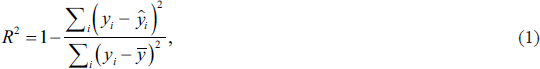
where
Comparison of Accuracy Across Different Sources.
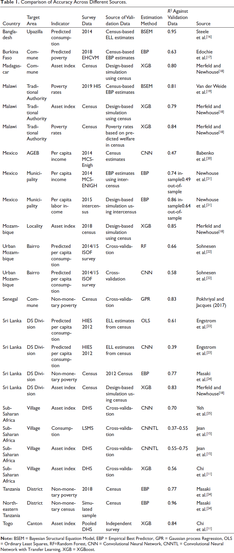
An important early paper on how geospatial data predict poverty and wealth was that of Jean et al.[15] Their paper used deep learning’ in the form of a convolutional neural network (CNN) to predict welfare, using daytime imagery taken from Google Earth and the luminosity of night-time lights in several countries in Sub-Saharan Africa. Each layer of the CNN successively filters the original image into more and more condensed abstract features, until the final layer represents the predicted luminosity value. Jean et al.[15] transfer the features from the penultimate layer of the CNN to a ridge regression that estimates the value of an asset index or per capita consumption in withheld villages.
In Jean et al.,[15] the target areas are survey clusters, the reference measure
Babenko et al.[20] improved upon this method by using daytime imagery to train a CNN model directly using survey data on per capita income. They trained the CNN model to predict the share of the population in extreme and moderate poverty in different Area Geo Estadistica Basicas (AGEBs)—small areas analogous to a census block—based on per capita income data collected in the 2014 MCS-ENIGH household survey. The prediction of AGEB-level poverty rates achieved an R2 of 0.47 when compared with survey estimates from withheld AGEBs. Interestingly, this is within the range reported by Jean et al.[15] for per capita consumption, despite the difference in welfare measure (income vs consumption) and country context. A prediction model based solely on land-cover classification predicted equally well, however, and models that used both predicted poverty (from the CNN) and the land-cover classification achieved an R2 of 0.57. This suggests that the CNN-based estimates of poverty in this case did not capture all of the imagery features correlated with average household per capita income. We further touch on the differences between interpretable and CNN-derived features below.
Newhouse et al.[21] use the CNN poverty estimates and land-cover classification from Babenko et al.[20] as inputs into empirical best predictor (EBP) models to predict poverty at the municipality level. The EBP model provides a simple framework for combining the two features in a linear mixed model, in addition to offering a well-established parametric bootstrap method for estimating uncertainty.[26] Official estimates for municipalities developed by the government based on the household-level intercensus were used as the reference for comparison. The R2 of the estimates was 0.74 for sampled municipalities but only 0.49 for non-sampled municipalities. Because this is only based on one sample, the paper also performed design-based simulations using a measure of per capita labour income taken from the intercensus. In the simulations, the R2 was 0.86 for sampled areas and 0.64 for out-of-sample areas. This article further discusses the difference in accuracy between sampled and non-sampled areas below.
Steele et al.[16] predict a wealth index and per capita expenditure in Bangladesh using a hierarchical Bayes structural equation model, allowing for spatial covariance. Their paper differs from many others by also incorporating CDR features from mobile phones in addition to satellite features. Results were validated both using cross-validation and using poverty estimates derived from the 2012 census. The results showed that it is much easier to predict wealth than per capita consumption, a finding consistent with Jean et al.[15] When using cross-validation for evaluation, out-of-sample R2 for village-level estimates was 0.76 for wealth as opposed to 0.36 for consumption. However, when comparing Upazilla-level (sub-district level) estimates with previous estimates derived using traditional small area estimates from the 2010 census, R2 was a much higher 0.95.
Similarly, Pokhriyal and Jacques[27] combine CDR and satellite data from Senegal with census data to predict non-monetary poverty across communes in Senegal. They use Gaussian process regression, a non-parametric machine learning method. They evaluate their estimates using 10-fold cross-validation. The estimates for non-monetary poverty across Communes achieved an out-of-sample R2 of 0.83 and a rank correlation of 0.87.
Chi et al.[11] used several DHSs and a mix of publicly available and proprietary geospatial data to predict an asset index for 2.4 km grids across 135 countries. The authors trained the model on the asset index available in the DHS, using data for 56 countries. Proprietary predictors include internet connectivity information obtained from Meta. In validation exercises, R2 varied greatly, depending on the context, level of geographic disaggregation, and comparison indicator. When validated using cross-validation across enumeration areas in the survey data, the R2 of the estimates was 0.56, similar to the 0.6 value reported by Yeh et al.[25] for Africa. Meanwhile, when validated against independent wealth measures, R2 was 0.60 across rural Kenyan villages, 0.70 across Nigerian Local Government Areas and 0.84 across Togolese Cantons. But when validated against the predicted probability of being poor, or predicted per capita consumption or income, R2 values are much lower: 0.04 across Malawian villages, 0.17 in Rural Kenya and approximately 0.3 across Mexican municipalities.[11, 21, 28] This is due to key differences between wealth and predicted per capita consumption, including the fact that the latter is expressed in per capita terms.
Masaki et al.[24] also consider the prediction of non-monetary poverty in Tanzania and Sri Lanka. Their study used census data from both countries to construct a non-monetary welfare index, and classified households whose index fell below a percentile threshold roughly equal to the prevailing national poverty rate as non-monetarily poor. The analysis combines survey-based estimates with publicly available geospatial indicators using an EBP model following.[2] Relative to direct survey estimates, the correlation with the census rose from 0.72 to 0.88 in Sri Lanka and from 0.77 to 0.88 in Tanzania. Unlike previous papers integrating survey and geospatial data, this one estimates the efficiency gain as well as the gain in accuracy due to incorporating geospatial data and finds that it is roughly equivalent to expanding the size of the sample by a factor between 3 and 5.
Van der Weide et al.[19] generate small area estimates of monetary poverty in Malawi for traditional authorities by combining survey data with publicly available geospatial features. Like Steele et al.,[16] their study uses a Bayesian structural equation model that accounts for spatial correlation across areas and validates the prediction against census-based estimates. It finds a correlation between the geospatial and census estimates above 0.9, although some individual target areas show substantial discrepancies between the census and geospatial-based estimates due to differences in the data used for prediction.
Krennmair and Schmid[29] propose a mixed effect random forest model, which is tested in a design-based simulation using household-level covariates in Mexico. The results demonstrate the benefits of applying machine learning methods over traditional linear models. Design-based simulations from the Mexican state of Nuevo León indicate that this approach reduces median relative bias by about 20% relative to the more typical approach of applying an EBP model with a transformation. The paper also evaluates a random effect block residual bootstrap approach to estimating uncertainty and finds that it performs well.
Merfeld and Newhouse[18] evaluate small area estimates of an asset index for four countries: Madagascar, Malawi, Mozambique, and Sri Lanka. In addition, the paper evaluates small area estimates of poverty for Malawi obtained using publicly available geospatial auxiliary data. This study compares linear EBP models with three different types of machine learning models: Extreme Gradient Boosting, Boosted Regression Forests, and Cubist regression. Unlike Krennmair et al.,[30] the machine learning models do not include a conditional random effect. Despite that, the results indicate that all three machine learning methods generate substantially more accurate estimates than the linear EBP model, particularly out of sample. Of the machine learning methods, boosted regression forests and extreme gradient boosting perform equally well except in Sri Lanka, where extreme gradient boosting produces slightly more accurate estimates. The random effect block residual bootstrap approach proposed by Krennmair et al.[30] also works well when applied to gradient boosting, providing coverage rates ranging from 94% to 97%.
Sohnesen et al.[22] evaluate small area estimates of proxy means test (PMT) scores in urban Mozambique using cross-validation methods. The paper shows estimates of the accuracy of random forest models based on OpenStreetMap (OSM) data on roads and distance to city centre as well as the density and structure of buildings. They find that this method predicts well, with out of sample R2s of 0.58 at the 115 × 115 m2 cell level and 0.66 when cells are aggregated to Bairros, a highly disaggregated administrative unit.
Finally, Lee and Braithwaite[31] propose an innovative iterative process that combines tree-based machine learning and deep learning to generate wealth estimates. This article first trains a model using extreme gradient boosting to predict the probability of being in different wealth classes using interpretable geospatial features, and then uses the predicted values from this procedure to train a CNN on satellite imagery. The predicted probabilities of being in different wealth classes from the CNN are subsequently fed back into the boosting model. This process is repeated iteratively until there is convergence. This improves upon the methodology in Jean et al.[15] by avoiding the use of night-time lights to train models. The authors report that the average out-of-sample R2 from withheld countries is 0.90.
In general, several studies suggest that small area estimates generated by combining survey and geospatial data are more accurate than those based solely on survey data, sometimes by significant margins. This is notable because small area estimates based on geospatial data are subject to model bias; for example, a model that uses night-time lights as a predictor may underestimate poverty in a poor area that happen to contain a highway, if the high level of night-time lights associated with highways makes the area look less poor from the sky than it actually is. However, at least when predicting poverty rates at higher levels such as subdistricts, the evidence so far indicates that model-based estimates based on geospatial indicators are more accurate than direct survey estimates. This implies that the benefits of reducing sampling error by supplementing survey data with model-based predictions derived from geospatial indicators outweighs the introduction of model bias.
Geospatial Data Are a Second-best Option When Recent Census Data Are Unavailable
Although geospatial data are strongly correlated with welfare across space, recent census data remain the gold standard for auxiliary data for small area estimation. Unfortunately, in many cases census data are old or unavailable, which creates two problems. First, because survey and census data cannot typically be linked at the household level to preserve confidentiality, it is standard when estimating a unit-level model to assume that the predictors follow the same distribution in the survey and the census data. This assumption becomes less tenable as the temporal gap between the census and survey increases. If the census and survey distributions are sufficiently different, estimating a linked model with primary-sampling-unit-level (PSU) aggregates from the census is preferable to assuming a common distribution.[32] A second and more important problem is that old census data, even if they are linked directly to the survey data, cannot reflect any changes that affect wealth or poverty that occurred since the census. Current geospatial data may be more likely to reflect current conditions than old census data, especially when including geospatial indicators such as precipitation and vegetation that better predict short-run shocks.
When it comes to census data, how old is too old? Or, put another way, at what age do census-based predictions become less accurate than current geospatial predictions? It is difficult to know, but Newhouse et al.[21] offer one small piece of evidence on this point. When evaluated against Mexican 2015 small area poverty estimated based on the intercensus, 2010 census-based estimates are more accurate than 2015 estimates based on geospatial indicators (correlation of 0.91 vs 0.86). However, this is only representative of one context, and regional patterns of poverty in Mexico may have been more static during this time than in other contexts.
Prediction Accuracy Is Very Sensitive to the Training Data
Many of the papers discussed above predict poverty rates or average asset indices estimated at the village level. Since these are often derived from surveys with a limited number of observations per village, this raises the issue of noise in the dependent variable. In fact, correlations between predicted values and census-based estimates depend critically on the extent of noise in the training data, which will reduce measured accuracy. For example, Engstrom et al.[23] considered how the accuracy of predictions depends on the size and nature of the sample used to estimate average per capita consumption at the GN division level. That analysis correlated interpretable geospatial features with predicted per capita consumption imputed into a census. Model R2 fell from 0.61 when using the mean over all census households, to 0.55 when using the mean over thirty households, and further to 0.40 when taking the mean over 8 households per enumeration area. Differences in the extent of noise present in the training data, as well as the reference evaluation measure, will not necessarily affect the ranking of different types of models within the same context. But it explains much of the wide variation in R2 observed in Table 1 across different studies, which underscores the benefits of evaluation studies that compare different methods in the same context, using the same reference measure.
Gualavisi and Newhouse[28] offer another stark example of how sensitive predictive accuracy is to the source of training data. Using a census extract from 10 districts in Malawi, the analysis compared estimates of average village welfare imputed into a household census with estimates derived from combining a survey with publicly available geospatial indicators. However, it also considers a third option, which involves hypothetically supplementing the survey with a partial registry, a microcensus’ that interviews all households in a randomly selected 450 of the 4,500 villages with geolocated data. This involves a two-step approach, where welfare is first predicted into the partial registry and then a geospatial model is trained against the partial registry predictions.
Using a partial registry in this way yields an R2 of 0.35, as opposed to 0.01 for the geospatial poverty map based on survey data and 0.02 for the wealth estimates from Chi et al.[11] These R2 values are much lower than those cited in the previous section. The weak correlation between the Chi et al.[11] estimates and these census-based predictions reflects the challenge of distinguishing between village welfare levels in this context. In particular, the sample consists of 4500 villages, in 10 poor Malawian districts, for which names could be matched between the census and the Unified Beneficiary Registry data containing household geocoordinates. In this context, the Chi et al.[11] estimates may perform poorly because they come from a model trained to wealth while the benchmark reference indicator is imputed per capita consumption; these are conceptually different measures of welfare that tend to diverge more in rural areas and among the extreme poor.[33] For the standard geospatial poverty map based on the survey, the low R2 is also due to the paucity of survey data, as there are only 16 households per enumeration area in the survey sample. Besides the disappointing performance of the standard geospatial poverty estimation and the Meta wealth index estimates in this challenging context, this exercise also illustrates how much the inclusion of additional data from the partial registry improves the performance of the prediction. The partial registry effectively adds valuable information to the training data when using geospatial data for small area estimation. This enables the development of a much more accurate prediction model, using proxy welfare variables that are cheaper and easier to collect.
The importance of training data raises the question of whether estimating different models for different geographies, such as urban and rural areas, improves prediction accuracy. Estimating separate models may improve the accuracy of the estimates by better accounting for heterogeneity across regions. However, these models also utilize less training data, which reduces the richness of the prediction model in the typical case when the sample is used to select or tune models. Newhouse et al.[21] provide some evidence on this question, comparing monetary poverty estimates in Mexico derived from a national model, separate models for urban and rural areas, and separate models for each of six state groupings. Compared to a baseline national model, estimating models separately for urban and rural areas leads to a minor improvement in accuracy, raising the correlation with census-based estimates from 0.86 to 0.87 in sampled areas and from 0.70 to 0.71 in non-sampled areas. Estimating separate models for six groups of states led to a similar minor improvement. These findings for Mexico, however, do not necessarily generalize to other contexts, and additional evidence comparing the accuracy of models specified at different levels would be useful. Tree-based machine learning methods, such as those discussed below, provide more flexible alternatives that explicitly model interactions between predictors. Use of these models should therefore mitigate any benefit from estimating multiple models in disaggregated geographic regions or areas.
Out-of-Sample Predictions Are Significantly Less Accurate Than In-Sample Predictions
Informative sampling occurs when sampling probabilities for primary sampling units vary in a way that is correlated with the outcome of interest, such as welfare. This is typically the case in two stage samples in which primary sampling units are sampled with probability proportional to size, since population size is correlated with most outcomes of interest. Informative samples, if not appropriately adjusted, produce biased estimates. The standard approach to adjust for informative sampling is to weight observations by the inverse probability of selection. This is usually straightforward to do when estimating EBP models with household surveys containing sample weights, for example when using the R Povmap and Stata SAE software packages. This protects against bias from informative sampling within sampled areas, but not against bias in predictions for areas that are not included in the sample.[34] The bias in estimates for non-sampled areas can be severe. Table 2 shows evidence on the extent to which informative sampling leads to less accurate predictions in non-sampled areas. The extent of this bias appears to depend on the country context and the nature of the sample. In the examples reported in Table 2, the estimates in Burkina Faso appear as a particular outlier, with an out-of-sample R2 of 0.21. It is difficult to know exactly why the out-of-sample estimates for Burkina Faso are so inaccurate, but this likely reflects large differences in the relationship between covariates and predictors between sampled and non-sampled areas. In addition, the source of validation data in that case is model-based EBP estimates derived from the census, which are also subject to bias due to informative sampling when predicting out of sample.
Predictions Using Geospatial Data Are Much Less Accurate in Non-sampled Areas.
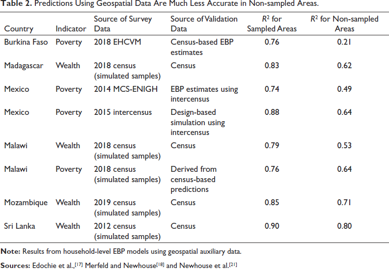
Pfeffermann and Sverchkov[35] proposed a bias correction for out-of-sample areas when the probability of selection of an area into the sample is known, but first stage sampling probabilities are rarely available to analysts, and this correction has not yet to our knowledge been implemented in any small area estimation software package. Estimating a separate model with inverse probability weighting for out-of-sample areas may have the potential to improve the accuracy of out-of-sample estimates, by giving greater weight to areas that were less likely to be sampled, based on observable characteristics, when estimating model parameters. As discussed in more detail below, tree-based machines learning methods are also more robust to this source of bias and therefore tend to generate more accurate out-of-sample predictions. Until either the use of tree-based machine learning or explicit bias correction becomes routine, however, predictions for out-of-sample areas based on publicly available geospatial indicators should be treated with great caution.
Predictions Across Time Are Much Less Accurate Than Predictions Across Space
In contrast to the many studies that have used satellite imagery to predict welfare levels across space, only two published studies to our knowledge have evaluated intertemporal predictions using geospatial data. Yeh et al.[25] attempt to use daytime imagery to predict changes in wealth measured in the DHSs. The CNN was only able to explain 15%–17% of the estimated changes across African villages, however. When using self-reported changes in assets from the most recent survey, the figure rose to 35%. When aggregating up to districts, and using self-reported changes from the endline survey, imagery can explain about half of the variation in self-reported changes. However, self-reported changes are subject to recall error and may only capture major changes in assets.
Meanwhile, Khachiyan et al.[36] look at variation across census blocks in the USA and find that a CNN trained on daytime imagery predicted half of the change in population density between 2000 and 2020, and 42% of the variation in income change between 2000 and 2017. Both Khachiyan et al.[36] and Yeh et al. (2020) use CNNs for prediction. Further studies would be very useful to test the ability of different methods and data sources to predict changes over time.
Summary of Key Lessons on Using Geospatial Data for Small Area Prediction
Overall, the main conclusion from this nascent literature is that geospatial data are strongly predictive of geographic variation in wealth and poverty. Exactly how predictive accuracy varies depending on a myriad number of factors. In general, wealth is easier to predict than consumption. Nonetheless, when national geospatial estimates of poverty or wealth are compared against census-based estimates for sampled areas, the R2 appear to consistently range from about 0.74 to 0.95, as shown in Table 1.
Because geospatial data are particularly predictive of population density[37, 38] and population density is systematically related to economic welfare (Castaneda et al., 2018),[64] geospatial data can help fill in’ two-stage household surveys with model-based predictions, boosting efficiency and accuracy. Most of the studies that have compared geospatial estimates with direct survey estimates find that the model-based estimates are more accurate, although the comparisons are not shown here. There is also evidence that prediction accuracy is highly dependent on the strength of the training data, suggesting that partial registries that collect proxy indicators may be a valuable supplement to household survey data when publicly available geospatial data can be linked. Finally, out-of-sample estimates are generally less accurate than in-sample estimates, and occasionally very inaccurate. This suggests that there are benefits from including as many target areas as possible in the sample, and from additional research and tools to improve out-of-sample prediction accuracy.
At the same time, the early literature has utilized a dizzying number of approaches to integrating survey and geospatial data. Many of these papers train a CNN model directly to imagery, others use machine learning methods applied to specific features, while others use linear mixed models. Those that either use deep learning or tree-based machine learning either ignore or may not properly estimate or evaluate uncertainty, and many of the papers ignore the well-established statistical literature on small area estimation. The following section explores these issues in greater detail.
Interpretable Features Predict at Least as well as Deep Learning from Imagery
One aspect in which the existing literature on geospatial data fusion has diverged involves the nature of the geospatial indicators used. While several studies obtain predictions directly from imagery using deep learning techniques such as CNNs, others instead generate predictions from interpretable features such as land classification types, night-time light luminosity, building density, and so on. When using interpretable features, predictions can be obtained using linear models—which may be regularized—or a tree-based machine learning algorithm such as extreme gradient boosting. It is possible to use both, as demonstrated in Lee and Braithwaite,[31] but using deep learning entails several additional costs. Deep learning models are complex and effectively a black box’ to users. Furthermore, they require specialized skills to understand and deploy, and thousands of training data points to perform well. On the other hand, the number of EAs in survey data are typically less than five hundred. Pre-trained CNNs can help circumvent the need for more data, but little is currently understood about how the specific nature of the architecture or pre-training affects prediction accuracy or bias.
A few existing studies shed light on the relative predictive power of deep learning and interpretable features. As noted above, Babenko et al.[20] compare the predictive power of poverty predictions obtained from a CNN, as well as with those obtained from land classification, and both together. The correlation with the benchmark measure of truth, derived from the census, was equally correlated with the direct CNNs and land classifications, and the correlation improved moderately when both were included.
Engstrom et al.[23] directly compare CNN-based estimates of headcount poverty rates with feature-based estimates in Sri Lanka. A variety of features were used, including roof type, shadows, cars, and road types. In that context, feature-based prediction is more accurate, with an R2 of 0.61 and a mean absolute error of 3.2 pp, as opposed to an R2 of 0.39 and a mean absolute error of 5.5 pp for the CNN-based estimates.
Ayush et al.[39] also derive several interpretable features such as trucks, maritime vessels, vehicles, aircraft, etc. They then compare predictions obtained from these features in a gradient boosting model with those obtained from a CNN trained to nightlights data, as in Jean et al.[15] When predicting average per capita consumption across villages, the out of sample R2 of the interpretable features is 0.54, as compared with 0.41 when using the CNN trained to night-time lights. While this is a lower bound measure of accuracy of the CNN, since it was trained to night-time lights, it is consistent with Engstrom et al.[23]
Sohnesen et al.[22] also compares the accuracy of estimates based on interpretable features with those derived from a CNN in urban Mozambique. The estimates based on interpretable features are based on a random forest model, and the interpretable features include information on buildings extracted from a CNN, as well as information on distance to different types of roads and the city centre taken from OSM. Despite the limited set of features, the feature-based approach substantially outperforms the estimates trained directly to a CNN. At the 115 × 115 m2 cell level, the feature-based approach gives an R2 of 0.58, as opposed to 0.38 for the CNN approach. When aggregated to Bairros, estimates based on features yield an R2 of 0.66, as opposed to 0.58 for the CNN-based approach.
Finally, as noted above, Lee and Braithwaite[31] employ an innovative approach that first uses interpretable features to predict the DHS wealth index, and then supplements that with poverty predicted from a deep learning model. This approach, however, shows limited benefits from adding direct CNN estimates to feature-based estimates for specific countries, with increases in R2 of only about 0 to 2 points across four of the five countries. The exception is South Africa, where there is an increase of about 8 points. These results also suggest that in many contexts adding deep learning estimates to existing predictions based on gradient boosting offers limited additional improvement in accuracy.
Household or Sub-area Models Are Usually Preferable to Area-Level Models When Sub-area Data Are Available
The pros and cons of different models for small area estimation in different contexts has been a subject of contention for many years and there is not yet a consensus between different statisticians and practitioners. For the purposes of this discussion, we assume that recent census data are unavailable, necessitating the use of geospatial data. In most cases, geospatial data are available in the form of zonal statistics at the sub-area level’, where the sub-area is a geographic area such as a grid or village. A zonal statistic, for example, could be the average night-time luminosity in the village or grid. Linking survey and geospatial data at the level of the enumeration area or village is quite common in practice. The DHSs publicly release jittered geocoordinates for each EA in most cases, facilitating this type of linking. Meanwhile, the target area is typically a more aggregate administrative unit, such as a district or subdistrict. Finally, we define the regional level as a level above the target area for which the survey is considered to be representative.
Many analysts use Bayesian modelling for small area estimation. We focus here, however, on EBP models,[2, 40] rather than purely Bayesian models, for three reasons. First, when they have been compared, EBP models give similar results to hierarchical Bayesian models.[41] Second, national statistics offices may be more comfortable with empirical Bayesian than Bayesian methods, partly due to discomfort with assuming a prior distribution. Finally, multiple well-documented and user-friendly software packages employ EBP methods, such as the EMDI, Povmap, and SAE packages in R, and the SAE package in Stata.[42–45]
Here, I focus on EBP models because they incorporate a conditional random effect that conditions on the sample, which is effectively used as a prior estimate. This distinguishes EBP models from two other popular alternatives: M-quantile (Chambers and Tzavidis, 2006)[65] and ELL.[3] Including a conditional random effect is particularly important when the auxiliary data are linked to the survey at the sub-area or area-level.[24] In this case, the sample contains more information relative to the auxiliary data than when using a typical household census, because the auxiliary data is identical for all households within a sub-area. This mechanically introduces correlation across households in a village, increasing the variance of the area effect. This in turn increases the weight given to the sample relative to the prediction in the EBP model when using aggregate predictors, as opposed to household-level predictors.
Within the set of EBP models, three main classes of model can be used to generate area-level poverty estimates using existing publicly available software packages.
The first type of EBP model for poverty estimation is a household-level model, as follows:

where
The assumption that the stochastic error terms are distributed normally necessitates transforming the dependent variable.[47] For household models, a log functional form has often traditionally been used, dating back to ELL.[3] But recently, a number of adaptive transformations that select a parameter to best fit the data have become increasingly popular, following their implementation in the publicly available EMDI software package. Examples of such adaptive transformations include the log-shift and Box-Cox transformations, in which a transformation parameter is selected through restricted information maximum likelihood. Newhouse et al.[21] and Masaki et al.[24] take a different approach, employing a rank order transformation that forces the dependent variable to follow a normal distribution, following Peterson and Cavanaugh.[48] While this does not guarantee that the residuals are normal, it brings them far closer to normality in those contexts. This transformation can be reversed under additional assumptions, although a back-transformation is not necessary for estimating headcount poverty.
The second type of model is a sub-area model’ specified at the lowest level at which the geospatial auxiliary data can be linked to the household model. This model assumes the form

where
The final option is to specify the model at the area level, which is the target area, following the long and distinguished literature spawned by Fay and Herriot[49]:

When testing the area-level models, we follow the recommendation of most software packages by specifying a simple version, namely a linear model with no variance smoothing. In particular, we obtain variance estimates for target areas by using the Horvitz–Thompson variance approximation. However, direct estimates of the variance at the target area level are imprecise, motivating the use of model-based small area estimation in general. Smoothing these variance estimates prior to estimation would likely generate more accurate predictions.[50, 51] In addition, accounting spatial and/or temporal correlation in a Fay–Herriot model can also improve prediction accuracy.[52, 53] A variant of the Fay–Herriot model that allows for spatial autocorrelation based on Petrucci and Salvati (2006)[66] has been implemented in the R EMDI package, while the R SAErobust package also implements the spatiotemporal correlation models proposed by Rao and Yu (1994)[67] and Marhuenda et al. (2013).[68] Testing area-level models with variance smoothing and spatial and temporal correlation structures against household and sub-area models that use sub-area predictors is a useful area for further research.
It is impossible to develop a general rule about the relative accuracy of different models, because their relative accuracy depends on the nature of the data. This is especially true when comparing across different sources of auxiliary data. For example, census data aggregated to the target area level may be preferable to geospatial data available at the sub-area level because it is more predictive of welfare, but current geospatial data may be preferable to old census data even if the latter is available at the household level.
Nonetheless, when considering a single source of auxiliary data, the household and sub-area models enjoy the important advantage of using auxiliary data at a more disaggregated level. The use of more spatially disaggregated data can lead to more accurate estimates of nonlinear functions such as headcount poverty rates, though these gains in accuracy may be negligible in some contexts. An additional benefit from using more spatially disaggregated estimates is the additional precision gained by exploiting the additional variation across sub-areas within areas. Whether the benefit comes in the form of increased accuracy, precision or both, when considering a single source of auxiliary data, it is generally preferable to use a household or sub-area model rather than an area-level model when possible.Although the general principle of using the most spatially disaggregated auxiliary data possible seems straightforward, there is not yet full consensus on this point in the literature. For example, Corral et al.[54] argue that, when considering model-based bias, household models with aggregate variables suffer from omitted variable bias, and therefore recommend using an area-level model rather than a household-level model when the auxiliary data consist solely of sub-area or area-level means. Newhouse et al.,[21] however, show that this source of omitted variable bias is equally present in area-level and household models that use auxiliary data drawn from the population, such as census or administrative data. Furthermore, this source of model-based bias disappears when considering design-model bias, taking the expected value of the predictions prior to drawing the sample. Omitted variable bias is therefore not a relevant concern when selecting between these different types of models.Corral et al.[55] nonetheless recommend the use of an area-level model rather than a household-level model when the predictors are available at the sub-area level, largely on the basis of results from a particular model-based simulation. This model-based simulation takes a simple random sample of households from all PSUs in the population. When the model-based simulation is altered to use a more realistic two-stage sample design in which a subset of PSUs are selected, the household model with sub-area means generates more accurate predictions than the area-level model.[1] Using a two-stage sample effectively increases sampling error in the direct estimates, which in turn increases the benefit of using more geographically disaggregated auxiliary data to fill in the geographic gaps of the sample. Using a one-stage sample, on the other hand, makes the direct survey estimates more accurate, which favours area-level models in this case. This partly illustrates why it is important to be careful before inferring general results from particular model-based simulations.[47]Relative to the area-level model, the household model benefits from using auxiliary data at the sub-area level. The greater variation of more spatially disaggregated data is particularly important when using algorithmic variable selection methods such as LASSO or stepwise regression to select models, which is increasingly common among practitioners. The availability of sub-area variation also becomes more important when forcing the model to include dummy variables at the regional level, the level for which the sample survey is considered to be representative. Forcing the inclusion of regional dummies in the model selection process generally increases the predictive accuracy of the model, by controlling for fixed characteristics of the region. In addition, including regional dummies enables model selection algorithms such as LASSO and stepwise to prioritize variables that best explain within-regional variation for inclusion in the model. Finally, since these algorithms use the sample to determine how many variables to select, using more disaggregated predictors ensures that a richer and more accurate predictive model is selected. The household model may also slightly benefit from predicting a continuous welfare variable, rather than discarding information—about how close a household is to the poverty line—by first converting it to an estimated headcount poverty rate, although it is not clear that this difference is important empirically. Table 3 shows empirical comparisons of accuracy, as measured by R2, from selected evaluations. R2 is shown because it is commonly reported and because its square root tends to be a good approximation of Spearman rank correlation, which is in turn useful for evaluating targeting performance.[2] In most cases, unfortunately, the evidence reported below is based on a single real-life survey. Only in Mexico, to our knowledge, is there simulation evidence comparing area and household-level models using geospatial auxiliary data. In each case, models are selected using LASSO and regional dummies are included.In general, the household model predicts more accurately than the area-level model in contexts where they have been directly compared against census data. The one notable exception is out-of-sample areas in Burkina Faso. However, for in-sample areas the household level model is significantly more accurate, such that the household-level model is more accurate overall (results not shown). In Tanzania, the area-level model also generates slightly more accurate predictions than the household-level model, although the difference is negligible. Interestingly, in the one simulation comparison in Mexico, the two models perform essentially equally well in-sample but the household model is moderately more accurate out-of-sample. Mexico also is different than the other cases in using a relatively small number of proprietary geospatial variables, which may also partly explain why estimates are far more accurate out-of-sample in Mexico than Burkina Faso. In addition, the simulation results reported for Mexico are based on area-level aggregates instead of sub-area level aggregates, due to the lack of sub-area identifiers in the census data. This may explain why the household model and area-level model perform equally well in sampled areas in this context.The comparisons reported in Table 3 are far from conclusive and should be interpreted with caution, since all except for one case are based on a single sample. In addition, the area-level models estimated here use direct survey estimates of variance as inputs into the model, obtained using the Horvitz–Thompson approximation of variance. As noted above, using smoothed variance estimates and accounting for spatial correlation should increase the accuracy of area-level models. Finally, the evaluation metrics are often themselves EBP estimates based on household census data, since official welfare measures are never observed in the census. Nonetheless, despite the limited evidence so far, the household level model appears to generate more accurate predictions than the area-level model in the majority of cases, sometimes by substantial margins. Additional evidence would be useful to get a better sense of the conditions under which household models or area-level models generate more accurate estimates.As noted above, a key benefit of incorporating sub-area level auxiliary data in a household model framework is increased efficiency. In Burkina Faso, the mean estimated mean-squared error for sampled areas was half as small when estimating a household model with sub-area predictors.[17] A similar 45% reduction in mean MSE was observed for in-sample municipalities in Mexico when incorporating sub-area level predictors.[21] While these are only two contexts, they suggest a large efficiency gain when using a household model with sub-area level predictors, relative to an area-level model.
R[2] by Method and In or Out of Sample, Relative to Validation Data.
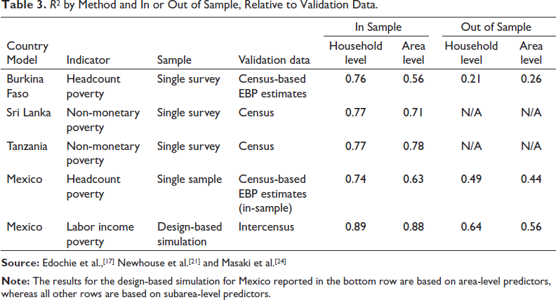
Another option is the sub-area level model given in equation (2), in which the unit of analysis is the sub-area and the dependent variable is sub-area-level poverty rates, in the spirit of Torabi and Rao (2014).[69] Unfortunately, there is little empirical evidence to our knowledge on the relative accuracy of estimates produced by a sub-area versus a household model. In Mexico, when using a single household survey sample, the R2 was equal to 0.70 relative to the evaluation benchmark, less than the 0.74 value for the household-level model. In Burkina Faso, again using a single household survey, the R2 of the sub-are model was 0.83 in-sample, 0.55 out of sample, and 0.77 overall, while the household model yielded an R2 of 0.87 in-sample, 0.45 out of sample, and 0.79 overall.[17] These results suggest that the household model may be if anything slightly more accurate than a sub-area model. These results only pertain to two contexts, however, and further research is needed to rigorously evaluate these different types of models.
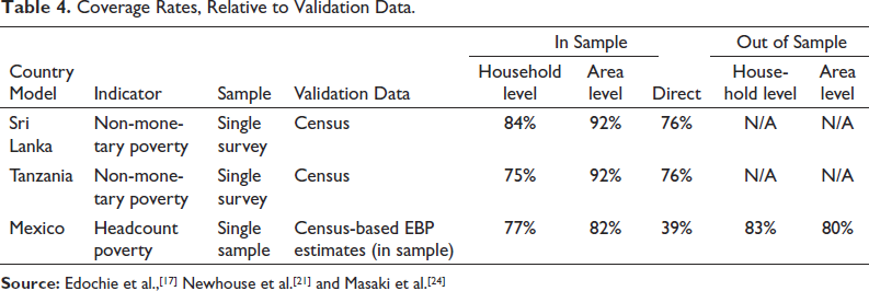
Many of the same studies also compare coverage rates across the models, which are useful for evaluating the accuracy of uncertainty estimates. If estimates of uncertainty are unbiased, coverage rates should be approximately equal to 95%. Table 4 lists estimated coverage rates from selected studies. When estimating the household model, confidence intervals are calculated based on mean squared error, under the assumption that the point estimates are unbiased. For estimating coverage rates, generally the area-level model fares better than the household model, providing coverage rates of 92% in Sri Lanka and Tanzania as opposed to 84% and 75% for the household model. The differences were more muted in Mexico, although unfortunately no coverage statistics were provided for the design-based simulation. The moderate underestimation of uncertainty in the household model may be due to the omission of a random effect at the sub-area level, although the direction of this bias due to omitting this sub-area random effect depends on the structure of the data (Marhuenda et al., 2017).[63] One way to get a sense of the magnitude of this downward bias in estimated uncertainty is to compare coverage rates with those of direct estimates. The standard cluster-robust variance estimator for surveys also underestimates uncertainty because it fails to account for the correlation in poverty status across enumeration areas within target areas. This leads to similarly low coverage rates for direct estimates in Sri Lanka and Tanzania, and much lower coverage rates in Mexico. When compared with the downward bias in standard direct variance estimates, the magnitude of the downward bias in the household model MSE estimates does not seem large enough to warrant serious concern. Tree-based machine learning methods appear to predict more accurately than linear models
Coverage Rates, Relative to Validation Data.
One of the key differences across the different studies listed in Table 1 is the choice of prediction method. Many of the studies used linear mixed models, drawing on the traditional methods popular in small area estimation. On the other hand, others use more sophisticated tree-based machine learning approaches such as Regression Forests or Gradient Boosting. Regression Forests are a generalization of decision trees. The take the average predictions of a continuous dependent variable over many decision trees, which are each derived from repeated random samples of the data and of candidate variables, a process known as bagging.[57] Bagging helps make random forests much more robust to small perturbations in the data than single decision trees. Extreme Gradient Boosting (XGboost), meanwhile, is a generalization of random forests.[58] This method generates predictions based on the sum of a sequence of regression forests, which are estimated by iteratively predicting the residual from the sum of the previous regression forests.
To our knowledge, Krennmair et al.[30] is the first paper to specify a model that combines a conditional random effect with tree-based machine learning, specifically random forests. When applied to Austrian income data, the mixed effect random forest model tends to generate more accurate predictions of mean income than traditional EBP. The authors conclude that random forest models offer substantial advantages over linear models in the presence of complex and non-linear interactions between covariates.
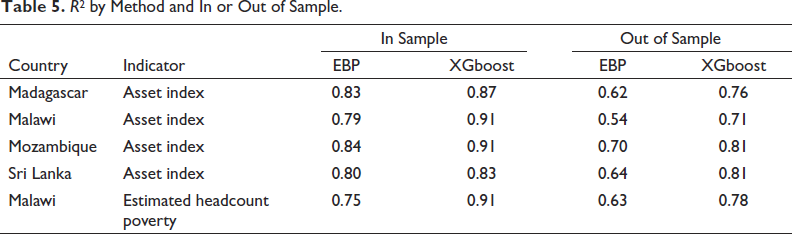
Merfeld and Newhouse[18] compare estimates produced using gradient boosting applied to geospatial data to those from a linear mixed effect EBP model, using samples containing 500 enumeration areas. This differs from Krennmair et al.[30] in two ways: It uses extreme gradient boosting instead of a single random forest model, and it assumes an unconditional random area effect instead of a conditional random area effect. The predictions are evaluated against census aggregates (for the asset index) or whether predicted welfare in the census falls below a threshold (for poverty in Malawi). Uncertainty is estimated using a block random effects bootstrap approach, as proposed by Chambers and Chandra[59] and applied in Krennmair et al.[30] The results in Table 5 show that XGboost, even without the conditional random effect, is more accurate than EBP in each case. For out-of-sample areas, the greater flexibility of the XGboost algorithm eliminates much of the selection bias associated with out-of-sample prediction using linear models under informative sampling. In results not shown here, coverage rates vary from 94% to 97%, reflecting the success of the bootstrap procedure in estimating uncertainty accurately.
R[2] by Method and In or Out of Sample.
A key application of small area estimation is assisting the identification of the poorest households through geographic targeting. Traditionally, cash transfer programs use Proxy Mean Tests (PMT) as a way to identify the poorest households, which utilize a registry of verifiable characteristics to assign each household a score.[60] The weight applied to each characteristic is typically determined through by regressing these proxy welfare indicators on log per capita consumption. However, registries are typically very costly and time-consuming to collect and update. In part because of this, recent research has explored the use of satellite and phone data as an alternative to identify poor households.
A recent paper[9] evaluates an innovative two-step approach to identify the poorest households in Togo, which was applied to the Novissi cash transfer program. The first step entailed using the Meta relative wealth index from Chi et al.[11] to identify the poorest hundred Cantons, which are the third administrative level in Togo, out of 397 total Cantons. Within these identified Cantons, the team used CDR data to identify poor households, using a model trained against per capita consumption collected as part of a phone survey in September 2020. Targeting accuracy was then evaluated against a Proxy Means Test constructed from an independent phone survey representative of all cell phone subscribers in the country.
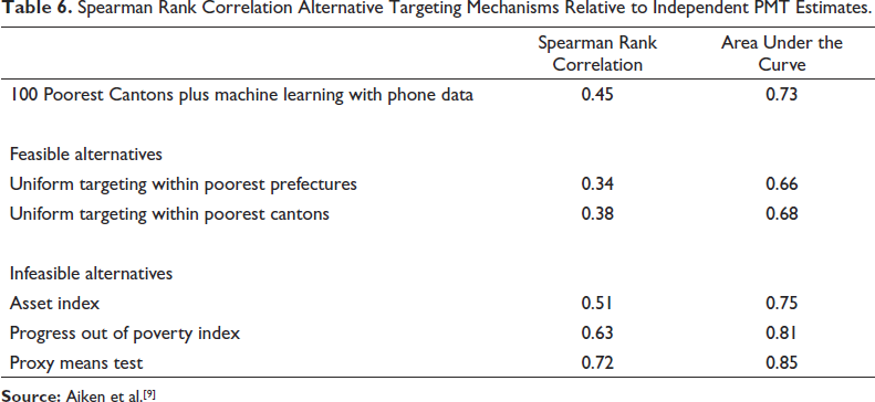
The headline result is that this two-step targeting approach outperformed two hypothetical feasible alternatives based on geographic targeting, as shown in Table 6. The first feasible alternative considered is a transfer of equal value to all persons within the poorest prefectures, which is the second administrative level in Togo, out of 40 total prefectures in Togo. The second alternative provided a transfer of equal value to all individuals within the poorest Cantons. Both of these hypothetical alternatives simulated transferring cash to all households in the poorest geographic areas, Prefectures in the first case and Cantons in the second, until 29% of the population was covered. This 29% threshold selected to cover the same percentage as the two-step approach that combined the relative wealth index with CDR data.
Spearman Rank Correlation Alternative Targeting Mechanisms Relative to Independent PMT Estimates.
Spearman Rank Correlation Alternative Targeting Mechanisms Relative to Independent PMT Estimates.
The Meta relative wealth index, however, is a measure of asset wealth rather than a measure of household-size adjusted consumption. This raises the question of whether targeting could be further improved if the 100 poorest cantons were identified using small area estimates of poverty, derived from combining survey and geospatial auxiliary data along the lines of the studies discussed above, instead of small area estimates of wealth. The paper does not address this question directly, because Canton-level poverty estimates derived from combining survey data on per capita consumption with geospatial data was not considered in the set of feasible options.
The first feasible alternative considered simulated the provision of a uniform transfer to all individuals within the poorest prefectures. There are only 40 prefectures in Togo, however, as opposed to 397 cantons. This means that the simulated prefecture transfer differs in two ways from the simulated Canton procedure. First, it is based on many fewer prefectures, which reduces targeting accuracy because no attempt is made to distinguish hypothetical recipients within prefectures. Secondly, the prefecture estimates are estimates of predicted per capita consumption instead of wealth, which all else equal should improve targeting, since a measure of predicted per capita consumption is used for evaluation. Comparing the bottom two rows in Table 6 indicates that in this case, targeting based on less wealthy Cantons is more accurate than targeting based on poor prefectures, as the benefits of more disaggregated targeting outweighs the disadvantage of targeting based on predicted wealth. However, this difference is not large, given the much smaller number of prefectures, as the difference in rank correlation is only 0.04. This suggests that geographic targeting could be further improved if the 100 poorest cantons were determined based on estimates of per capita consumption rather than wealth.
Thirty-five years after the publication of Battese, Harter and Fuller[1] and seven years after the publication of Jean et al.,[15] the literature on combining survey and geospatial data to predict wealth and poverty is maturing rapidly. It is clear that indicators derived from geospatial data are strongly predictive of wealth and poverty across space in several contexts, although the extent of this correlation depends on many factors. The accuracy of predictions, however, is particularly sensitive to the nature of the household data on welfare or wealth used to train the model. It is also clear that the coverage of the training sample also matters.
Estimates for out-of-sample areas are almost always less accurate than for in-sample areas, because informative sampling introduces bias, and because Bayesian and empirical Bayesian methods do not benefit from sample-based priors. In addition, the evaluation benchmark in out-of-sample areas, if it is a model-based estimate, will also be biased due to informative sampling. Finally, the few studies that have considered the prediction of changes over time have found that this is much harder than prediction across space, even for medium to long-run changes. Seeing short-run changes in the welfare from space may prove challenging but is a challenge worth taking on.
The recent literature has offered more discussion than evidence regarding the pros and cons of different methodologies. One dividing line has been the choice of direct CNNs’ trained directly to survey data as opposed to utilizing interpretable geospatial features in a mixed linear or tree-based machine learning model. In Uganda and Sri Lanka, where both approaches have been compared, it seems that the interpretable features approach does at least as well as training directly CNNs, but the evidence on this question remains scant. A second fault line has emerged over the level at which to specify linear models. As a general rule, predictions typically benefit from using the most spatially disaggregated data possible, so if sub-area level data are available, area-level models should be only used as a last resort. This is particularly true when considering an evaluation criterion that combines accuracy and precision, such as mean squared error, since the use of more granular auxiliary data appears to have a larger beneficial effect on precision than accuracy. More research can shed more light on the pros and cons of sub-area models’ that predict poverty rates with the sub-area as the unit of observation, vis-à-vis household level models with sub-area mean predictors, where repeated simulations are used to generate poverty estimates.
Finally, there are new developments applying tree-based machine learning techniques. These generally offer greater predictive power than linear models at the cost of parsimony and transparency.[61] Tree-based machine learning models are more robust to outliers, and less susceptible to bias arising from informative sampling when predicting out of sample. Two important obstacles to more widespread adoption of machine learning methods have recently been surmounted. The first was the lack of asymptotic theory. Asymptotic theory has, however, recently provided for generalized random forests, a large class of methods that includes boosted regression forests, which is a type of gradient boosting.[62] The second obstacle was the lack of an accepted method for uncertainty estimation. Although Athey et al.[62] developed methods to estimate uncertainty for boosted regression forests, the random effect residual bootstrap developed by Chambers and Chandra[59] and first applied by Krennmair and Schmid[29] is also an attractive and simple option that appears to work well for wealth prediction using extreme gradient boosting in multiple contexts.[18]
While the potential of regularly pairing survey data with geospatial data is clear, more work on research and tools is needed to further instil confidence in the estimates and facilitate use. Research could benefit from more comparative work on methods, ideally utilizing design-based simulations using georeferenced census data. These can examine several outstanding research questions, including the relative benefit of CNNs versus simpler estimation approaches, quantifying the benefits of including conditional random effects when using machine learning models, probing the robustness of methods for estimating the uncertainty associated with tree-based machine learning estimates, experimenting with different geospatial features, and determining the age threshold at which census-based estimates become less accurate than geospatial estimates in different contexts. The question of which features best predict changes is also important. For example, changes in the rate of building construction, the characteristics of new buildings, or changes in crop types and forecasted yields have not yet to our knowledge been tested as correlates of welfare changes.
In addition to further research, further improvements to open-source tools are critical to make these techniques more accessible and educate users. This is particularly important to facilitate the adoption of more sophisticated methods in developing countries given the financial and technical constraints faced by national statistical offices and other practitioners. The R EMDI, Povmap, SAE, SAEforest, and GRF packages available on CRAN are all examples of good practice, as the documentation for each is clear, comprehensive, and up to date. No such comparable user-friendly package exists for neural network models at this time. No matter how many new and improved methods are published by statisticians, they are unlikely to be used in practice without software that is accessible to non-specialists and thoroughly documented. User-friendly features automating common diagnostics and parallelizing across multiple cores to speed estimation, as implemented in the EMDI package, are very valuable. Finally, software that makes it simple to obtain and link publicly available geospatial indicators with survey data will also help facilitate data integration. As these tools are developed, small area estimates that combine survey data with publicly available geospatial data will inevitably become more popular worldwide, belatedly fulfilling the promise demonstrated thirty-five years ago by Battese, Harter and Fuller (1988).[1]
Footnotes
Acknowledgements
I would like to thank Partha Lahiri for suggesting this article, for offering the opportunity to present an earlier version at the 2022 Small Area Estimation conference at the University of Maryland College Park, and for his strong support of this research agenda. I would like to thank William Bell, Chris Elbers, Carolina Franco and Josh Merfeld for helpful comments on a previous draft. I am indebted to Haishan Fu, Keith Garrett, Dean Jolliffe, Talip Kilic, and Roy Van der Weide for helpful discussions and support for this line of research. I would like to thank many who collaborated on related work over the years, including Marshall Burke, Ify Edochie, Ryan Engstrom, Melany Gualavisi, Jon Hersh, Partha Lahiri, Taka Masaki, Josh Merfeld, Anthony Perez, Anusha Ramakrishnan, Utz Pape, Timo Schmid, Ani Silwal, Vidhya Soundararajan, Kibrom Tafere, Nikos Tzavidis and Michael Weber. This research is a product of the World Bank’s Development Economics Data Group.
Declaration of Conflicting Interests
The authors declared no potential conflicts of interest with respect to the research, authorship and/or publication of this article.
Funding
The authors received no financial support for the research, authorship and/or publication of this article.