Sage Journals: Discover world-class research

Abstract

Background

ML predictive models have shown their capability to improve risk prediction and assist medical decision‐making, nevertheless, there is a lack of accuracy systems to early identify future rapid CKD progressors in Colombia and even in South America.

Objective

The purpose of this study was to develop a series of interpretable machine learning models that predict GFR at 6-months, 9-months, and 12-months.

Study Design and Setting

Over 29,000 CKD patients stage 1 to 3b (estimated GFR, <60 mL/min/1.73 m²) with an average of 3-year follow-up data were included. We used the machine learning extreme gradient boosting (XGBoost) to build three models to predict the next eGFR. Models were internally and externally validated. In addition, we included SHapley Additive exPlanation (SHAP) values to offer interpretable global and local prediction models.

Results

All models showed a good performance in development and external validation. However, the 6-months XGBoost prediction model showed the best performance in internal (MAE average = 6.07; RSME = 78.87), and in external validation (MAE average = 6.45, RSME = 18.94). The top 3 most influential features that pushed the predicted eGFR value to lower values were the interpolated values for eGFR and creatinine, and eGFR at baseline.

Conclusion

In the current study we have developed and validated machine learning models to predict the next eGFR value at different intervals. Furthermore, we attempted to approach the need for prediction explanation by offering transparent predictions.

Keywords

Machine learning chronic kidney disease extreme gradient boosting risk prediction

Introduction

Chronic kidney disease (CKD) is considered a global public health problem, being one of the main contributing diseases to the global burden of non-communicable diseases.¹ It is associated with important serious outcomes including increased risk of mortality, accelerated cardiovascular disease, adverse metabolic and nutritional consequences, reduced cognitive function, and increased risk of acute kidney injury.²

CKD is a significant and gradual problem in low- and middle-income countries (LMICs) due to the increasing number of people with type 2 diabetes, hypertension, obesity, and vascular diseases.³ Besides, 63% percent of the global burden of CKD occurs in LMICs.⁴

In developing countries high mortality rates due to poor access to renal replacement therapy, as well as increased incidence of CKD, are expected to result in a substantial financial burden on health systems.⁵ In this regard, systematic approaches to detecting and monitoring CKD can substantially mitigate cardiovascular complications and delay the progression of end-stage renal disease.³

It is well known that inexpensive interventions can slow the rate of kidney function loss, consequently, there is some enthusiasm for population-based screening to allow early intervention in both low-income and high-income countries.⁶ Despite the growing burden of CKD in LMICs, few population-based screening models have been implemented at the national or local clinical level to specifically prevent or manage complications related to CKD.³

An approach that has been shown promising results, is risk stratification using machine learning (ML) techniques.⁷ Several studies have reported that machine learning outperforms conventional statistical methods due to its ability to better identify variables relevant to clinical outcomes and its better modeling of complex relationships.⁸ Furthermore, in healthcare is still a challenge to deal with the vast amount of data from different types of structures, a problem that machine learning techniques have proven to overcome because of its robustness to data noise and its ability to learn from multiple data sets.⁹

Considering that CKD is one of the highest costly diseases in Colombia and in Latin America, risk stratification models with few but sufficient predictors are highly desirable.^10,11 Further, a predictive model to estimate the next eGFR, using very few predictors, could be highly useful due to its ease of use in clinical practice, a greater possibility of reproducibility in other clinical contexts, and for the potential application of prediction in the design of targeted interventions.

In the present study, we developed interpretable prediction models for the next eGFR estimation. Using ML techniques incorporating a few clinical parameters, we developed and internally and externally validated ML models to predict the 6-months, 9-months, and 12-months eGFR value using data from a large cohort of Colombian CKD patients from the Caribbean region. This risk stratification system is designed to assist case managers and physicians in predicting CKD prognosis quickly and accurately.

Methods

Population - study cohorts

The retrospective cohort study was performed including a large CKD Colombian Caribbean Cohort coming from primary and secondary ambulatory care.

We used one observational study cohort derived from primary care records of a Colombian health service provider specialized in the treatment of chronic diseases. The cohort was composed of follow-up data from 29,447 patients with a diagnosis of CKD stages 1 to 3b (estimated GFR, <60 mL/min/1.73 m²) collected after 2017 (Mean of follow-up = 3 years). Records were extracted from the laboratory information system and electronic health records.

Records on the cohort were screened based on eGFR and were included after checking according to the eligibility and exclusion criteria. The key eligibility criteria were Colombian, 18–90 years, eGFR: >30 mL/min/1.73 m², and no initiation of renal replacement therapy (RRT). The key exclusion criteria were follow-up time <12 months, less than three outcome and predictor measurements during follow-up, diagnostic of Polycystic kidney disease (PKD), HIV, cancer treatment in the past 2 years, and renal transplantation, according to medical records.

The exclusion criteria were implemented to address specific limitations in the data provided by the healthcare provider for this study. In Colombia, healthcare providers often specialize in managing particular diagnoses or groups of related conditions. The provider that supplied our study database focuses on chronic diseases, including hypertension, diabetes, and chronic kidney disease (prior to renal replacement therapy). Patients with additional conditions such as HIV, cancer, or those undergoing renal replacement therapy are managed by other specialized providers. Consequently, follow-up data for these conditions are not included in the database provided. By excluding these cases, we aimed to reduce potential bias due to the unavailability of relevant data.

Outcome

The outcome variable was eGFR estimation at 6, 9, and 12 months, as a key clinical indicator of CKD progression. GFR was estimated using the Cockcroft‐Gault equation.¹² Therefore, the medical tasks that the model is intended to support are diagnostic staging and prognosis.

Candidate predictors

Candidate predictors were pre-identified from a literature review, and their face validity according to clinical expertise. Demographic variables such as age and sex were included as well as routine clinical variables such as body mass index (BMI), systolic blood pressure (SBP), diastolic blood pressure (SBP), type 2 diabetes, hypertension; and routine clinical laboratory variables (creatinine) and GFRe at different intervals.

Estimating values for prediction intervals

To estimate the value of each continuous variable at the end of the prediction period, we used linear interpolation based on the two closest available measurements. This method applied to serum creatinine, blood pressure (both systolic and diastolic), BMI, and GFR to model how these variables change over time.

We began by taking a measurement from the start of the observation period (baseline) and another from the end of this period (beginning of the prediction period). The observation period is the time before the prediction period when data was collected to forecast the next GFR.

The linear interpolation was performed using the formula: $y = \frac{(x - x 1)}{(x 2 - x 1)} (y 2 - y 1) + y 1$ .

For example, to estimate the serum creatinine value at the start of the prediction period:

• y1 is the serum creatinine value closest to the start of the prediction period (0.80 mg/dL).

• y2 is the serum creatinine value closest but later than y1 (0.70 mg/dL).

• x is the start of the prediction period (March 2, 2022).

• x1 is the most recent date before the prediction period (February 22, 2022).

• x2 is the first date after the prediction period (March 18, 2022).

Then,

y = \frac{(2 - 03 - 2022 - 22 - 02 - 2022)}{(18 - 03 - 22 - 22 - 02 - 2022)} (0.70 - 0.80) + 0.80

y = 0.76 mg/dL, is the interpolated creatinine value.

The interpolation method using only two values was chosen considering the data availability scenario in a low- and middle-income country (LMIC) like Colombia. In clinical settings, the availability and frequency of measurements can vary significantly. Therefore, a method that is broadly applicable, even in scenarios with minimal data points, is more suitable. By relying on two points, this method can be applied consistently across different patient records, including those with sparse data.

Internal and external validation samples

The development cohort was composed of follow-up data from 11,730 CKD patients for the 6-month prediction model (mean age: 66.18; 68.52% women), 9,974 patients for the 9-month prediction model (mean age: 66.43; 68.28% women), and 8,191 patients for the 12-month prediction model (mean age: 66.57; 68.25% women).

The external validation cohort for the 6-month prediction model included 2,933 CKD patients (mean age: 66.69; 68.80% women), 2,494 patients for the 9-month prediction model (mean age: 65.99; 70.44% women), and 2,048 patients for the 12-month prediction model (mean age: 66.54; 69.67% women).

The external validation cohort consisted of a sub-sample of the Caribbean region cohort, which was not used during model training. Although this cohort is derived from the same overall population, it includes data from different healthcare centers located in various cities across the Caribbean region of Colombia, introducing variability in clinical practices and patient demographics. This diversity allows the external validation cohort to function effectively as an independent dataset, assessing the model’s generalizability in a slightly different context.

All patients were from 8 healthcare centers focused on primary and secondary care, located in different cities across the Caribbean region of Colombia. Figure 1 shows the workflow process of patient inclusion and exclusion.

Figure 1.

Work-flow process of inclusion-exclusion of patients in both cohorts.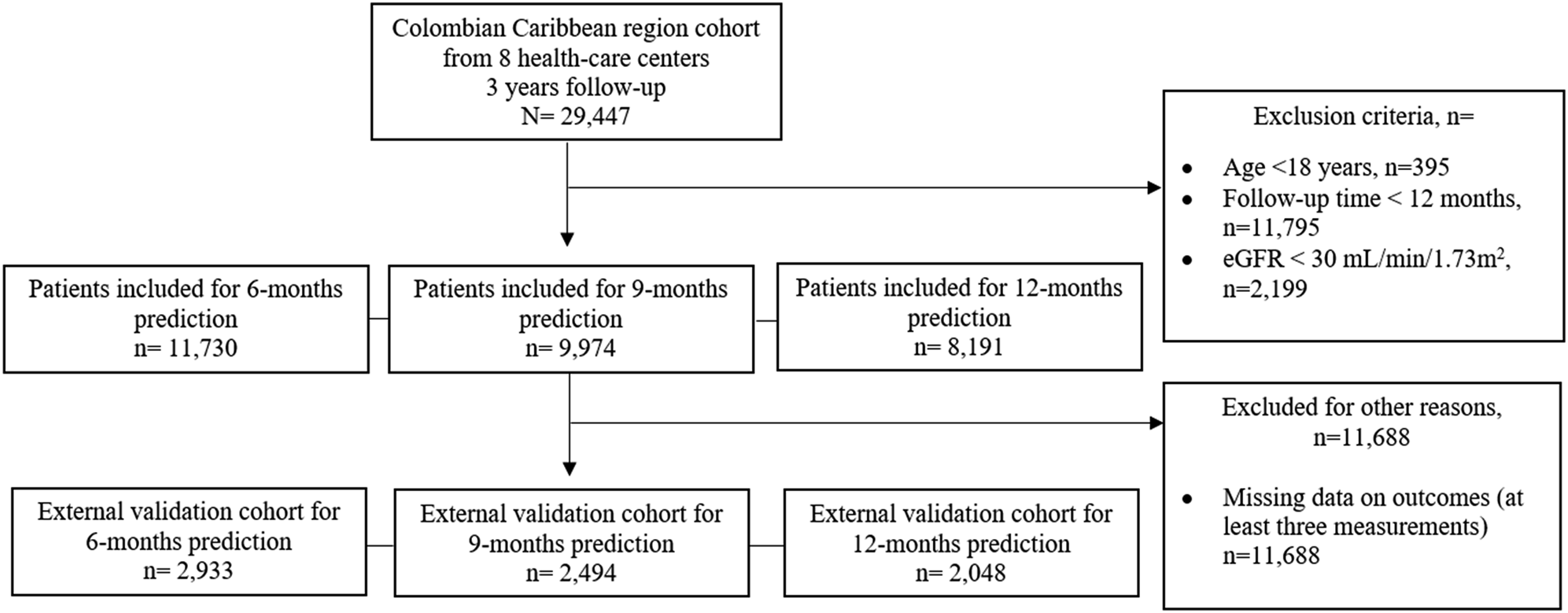

Models developing

Variables with more than 30% missing values were excluded from the analysis. Bivariate analyses were conducted using Student’s t-test and the χ² test to assess differences across cohorts, with a significance level of 0.05. These statistical analyses were conducted in Python.

We trained a series of linear regression models using eXtreme Gradient Boosting (XGBoost) to predict the next eGFR value. XGBoost is a machine learning technique that constructs an ensemble of decision trees to build a predictive model. During training, it iteratively generates new decision trees to correct errors from the current model, improving the prediction of the outcome variable. The final output is the cumulative score of all decision trees, representing the predicted outcome likelihood.

XGBoost offers a significant advantage over other machine learning techniques due to its scalability. It can run more than ten times faster than existing popular solutions on a single machine and scales effectively to billions of examples in distributed or memory-limited settings.¹³

Model performance was evaluated using three metrics:

• Mean Absolute Error (MAE): Measures the average absolute difference between predicted and observed values, reflecting the average prediction error.

• Root Mean Squared Error (RMSE): Assesses the square root of the average squared differences between predicted and actual values, emphasizing larger errors.

• R-squared (R²): Indicates the proportion of variance in the outcome variable explained by the model.

These metrics were used to assess the accuracy and robustness of the XGBoost models trained to predict eGFR. For external validation, the Relative RMSE (RMSE/SD) was also reported to normalize the RMSE relative to the variability in the data.

Parameters for the XGBoost algorithm were optimized using a grid search over 3,456 models with 3-fold cross-validation. The grid search included the following parameter ranges: the learning rate was set from 0.0001 to 0.1, the number of boosted trees (n_estimators) ranged from 50 to 500, the subsample parameter (to add randomness and robustness to noise) ranged from 0.6 to 1.0, and the maximum depth of a tree (to reduce model complexity) was set to either 3 or 4. The specific parameter grid is shown below: grid_param = {

“min_child_weight”: [1, 5, 10],

“gamma”: [0.5, 1, 1.5, 2],

“subsample”: [0.6, 0.8, 1.0],

“colsample_bytree”: [0.6, 1.0],

“max_depth”: [3, 4],

“n_estimators”: [50, 100, 200, 300, 400, 500],

“learning_rate”: [0.0001, 0.001, 0.01, 0.1]}

A total of 3,456 combinations (3 × 4 × 3 × 2 × 2 × 6 × 4) were tested.

To address class imbalance during model training, we analyzed class distributions and used XGBoost’s inherent class weighting capabilities to adjust the impact of imbalanced classes. The scale_pos_weight parameter was configured to account for class imbalance. Additionally, we monitored model performance metrics, including MAE, RMSE, and R-squared, to ensure effective model fitting and assess the influence of any class imbalances.

All analyses were conducted in Python using xgboost v. 1.5.2, shap v. 0.40.0, and scikit-learn v. 1.0.1 packages.

Internal and external validation

For internal validation, datasets were randomly split into training and testing datasets for each interval: 6 months (training n = 11,730, testing n = 2,933), 9 months (training n = 9,974, testing n = 2,494), and 12 months (training n = 8,191, testing n = 2,048). Additionally, the best-performing prediction models in the internal validation dataset were evaluated in external datasets.

Interpretability of models

Since the target users of the described models are clinicians and hospital management teams, we made efforts to include a way of visualizing the model results. To enhance the interpretation of the models, mitigate the black-box issue associated with ML techniques, and improve clinical usability, we employed the Shapley Additive exPlanations (SHAP) method.¹⁴

SHAP is a Python framework designed for explaining the output of any machine learning model using classical Shapley values from game theory. It leverages a combination of feature contributions and Shapley values to generate SHAP values, quantifying the contribution of each feature to the prediction. Additionally, SHAP calculates global feature importance by averaging the magnitudes of the SHAP values across the dataset.¹⁵

The SHAP approach provides both global and local interpretability of each model. It highlights the importance of each predictor feature globally and indicates the importance relative to a specific individual locally. SHAP explains the model’s outcome as the sum of each contributing variable. A value greater than zero signifies that the variable increases the predicted outcome for the individual, while a value less than zero indicates the opposite.¹⁶

This study adhered to the principles outlined in the Declaration of Helsinki. Written informed consent was not necessary since the data were extracted from medical history records, and the analysis did not include identifiable information (Health Insurance Portability and Accountability Act Privacy Rule).¹⁷ Therefore, approval from the institutional review board was not required for this study.

Furthermore, this report follows the comprehensive checklist for the (self)-assessment of medical AI studies.¹⁸

Results

Continuous variables are presented as median, range, mean ± SD, and categorical variables as absolute frequencies and percentages (n, %). The bivariate analysis did not show a statistical difference across baseline measures between cohorts (P > .05). Table 1 shows the baseline characteristics of CKD patients across the development and validation cohorts.

Table 1.

Baseline characteristics of development and external validation cohorts.

	6-months		9-months		12-months
Variables	Development cohort (N = 11730)	External validation cohort (N = 2933)	Development cohort (N = 9974)	External validation cohort (N = 2494)	Development cohort (N = 8191)	External validation cohort (N = 2048)
Age	Mean: 66.18	Mean: 66.69	Mean: 66.43	Mean: 65.99	Mean: 66.57	Mean: 66.54
	SD: 14.72	SD: 14.74	SD: 14.50	SD: 14.83	SD: 14.52	SD: 14.63
	Median: 67	Median: 67	Median: 67	Median: 67	Median: 67	Median: 67
	Range:104	Range: 103	Range:103	Range:103	Range:103	Range:102
Sex	Female: 8038– 68.52%	Female: 2018 – 68.80%	Female: 6811 – 68.28%	Female: 1757 – 70.44%	Female: 5591 – 68.25%	Female: 14.27 – 69.67%
	Male: 3692- 31.47%	Male: 915–31.19%	Male: 3163 – 31.71	Male: 737 – 29.55%	Male: 2600 – 31.74%	Male: 621 – 30.32%
	Missing: 0 - 0%	Missing: 0–0%	Missing: 0 – 0%	Missing: 0 – 0%	Missing: 0- 0%	Missing: 0 – 0%
BMI	Mean: 26.56	Mean: 26.52	Mean: 26.61	Mean: 26.60	Mean: 26.57	Mean: 26.67
	SD: 4.50	SD: 4.58	SD: 4.50	SD: 4.53	SD: 4.46	SD: 4.59
	Median: 26.30	Median: 26.22	Median: 26.38	Median: 26.32	Median: 26.36	Median:26.48
	Range: 31.91	Range: 29.46	Range: 29.46	Range: 28.23	Range: 29.30	Range: 28.05
Serum creatinine, mg/dL	Mean: 1.02	Mean: 1.01	Mean: 1.01	Mean: 1.01	Mean: 1.02	Mean: 1.01
	SD: 0.30	SD: 0.28	SD: 0.29	SD: 0.28	SD: 0.29	SD: 0.29
	Median: 0.96	Median: 0.96	Median: 0.96	Median: 0.95	Median: 0.96	Median:0.96
	Range: 4.62	Range: 3.3	Range: 4.62	Range: 2.76	Range: 4.62	Range: 3.32
Diastolic blood pressure	Mean: 78.19	Mean: 78.08	Mean: 78.41	Mean: 78.16	Mean: 78.52	Mean: 78.40
	SD: 9.11	SD: 9.10	SD: 8.92	SD: 8.81	SD: 8.73	SD: 8.65
	Median: 80	Median: 80	Median: 80	Median: 80	Median: 80	Median:80
	Range: 65	Range: 60	Range: 59	Range: 55	Range: 56	Range: 52
Systolic blood pressure	Mean: 127.16	Mean: 127.30	Mean: 127.18	Mean: 126.51	Mean: 126.97	Mean: 126.42
	SD: 15.31	SD: 15.29	SD: 15.13	SD: 14.58	SD: 14.87	SD: 14.61
	Median: 120	Median: 120	Median: 120	Median: 120	Median: 120	Median: 120
	Range: 108	Range: 108	Range: 108	Range: 100	Range: 108	Range: 100
eGFR, mL/min/1.73 m2	Mean: 66.89	Mean: 66.42	Mean: 66.72	Mean: 66.88	Mean: 66.39	Mean: 66.21
	SD: 33.77	SD: 27.37	SD: 34.37	SD: 27.58	SD: 35.73	SD: 27.00
	Median: 62.76	Median: 62.39	Median: 62.75	Median: 62.79	Median: 62.26	Median: 62.04
	Range: 140	Range: 140	Range: 140	Range: 140	Range: 140	Range: 140
Type 2 Diabetes	0: 6537– 55.72%	0: 1652–56.32%	0: 5703 – 57.17%	0: 1420 – 56.93%	0: 4673 – 57.07%	0: 1180 – 57.61%
	1: 4198–35.78%	1: 1029–35.08%	1: 3450 – 34.58%	1: 889 – 35.64%	1: 2926 – 35.72%	1: 741 – 36.18%
	Missing: 995–8.48%	Missing: 252- 8.59%	Missing: 821 – 8.23%	Missing: 185 – 7.41%	Missing: 592 – 7.22%	Missing: 127 – 6.20%
Hypertension	0: 1340–11.42%	0: 327–11.14%	0: 1071 – 10.73%	0: 271 – 10.86%	0: 911–11.12%	0: 208–10.15%
	1: 9395–80.09%	1: 2354–80.25%	1: 8082 – 81.03%	1: 2038 – 81.71%	1: 6688–81.65%	1: 1713–83.64%
	Missing: 995 –8.48%	Missing: 252–8.59%	Missing: 821 – 8.23%	Missing: 185 – 7.41%	Missing: 592–7.22%	Missing: 127 – 6.20%

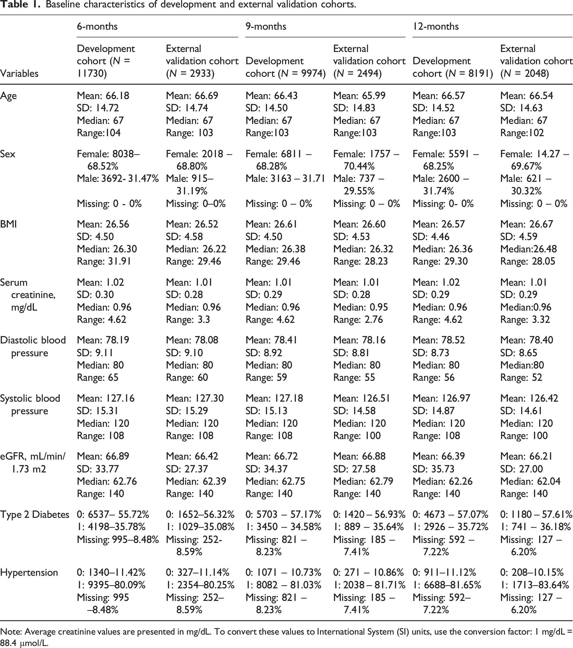
Note: Average creatinine values are presented in mg/dL. To convert these values to International System (SI) units, use the conversion factor: 1 mg/dL = 88.4 μmol/L.

The XGBoost model for prediction at 6-months had the best performance in training dataset (MAE average = 6.07; RSME = 78.87), and in testing dataset (MAE average = 6.73; RSME = 799.47) compared with model at 9-months (MAE average training dataset = 7.84, RSME = 125.57; MAE average testing dataset = 6.73, RMSE = 799.47) and with model at 12-months (MAE average training dataset = 7.80, RSME = 190.4; MAE average testing dataset = 8.14, RMSE = 128.73).

In external validation datasets the performance was quite similar for the model at 6-months prediction (MAE average = 6.45, RSME = 18.94, RMSE/SD = 0.722, R² = 0.47), at 9-months prediction (MAE average = 6.45, RSME = 361.89, RMSE/SD = 0.398, R² = 0.84), and at 12-months prediction (MAE average = 8.33, RSME = 378.23, RMSE/SD = 0.408; R² = 0.83).

Table 2 shows the most contributing attributes across the models being eGFR – interpolated the most important feature in all models. For instance, for prediction at 6-months the most important features were eGFR – interpolated, eGFR at baseline, sex, BMI – interpolated, and age. For the 9-months prediction model the most important attributes were eGFR – interpolated, diastolic blood pressure at baseline, eGFR at baseline, and BMI – interpolated. Finally, for the 12-months prediction model the most important attributes were eGFR – interpolated, BMI – interpolated, eGFR at baseline, and BMI at baseline.

Table 2.

Predictors selected using XGboost and their importance score for eGFR estimation models.

Predictors	Importance score
Predictors	6 Months	9 Months	12 Months
Sex	0.0202	0.0145	0.0023
Age	0.0188	0.0220	0.0139
Type 2 Diabetes	0.0099	0.0130	0.0021
Hypertension	0.0113	0.0105	0.0000
Creatinine (mg/dL) at baseline	0.0132	0.0107	0.0046
Creatinine (mg/dL) - interpolated	0.0147	0.0440	0.0058
BMI at baseline	0.0119	0.0743	0.0442
BMI - interpolated	0.0205	0.0841	0.2497
Diastolic blood pressure at baseline	0.0086	0.0948	0.0109
Diastolic blood pressure - interpolated	0.0098	0.0717	0.0027
Systolic blood pressure at baseline	0.0111	0.0105	0.0061
Systolic blood pressure - interpolated	0.0085	0.0088	0.0074
eGFR at baseline	0.0322	0.0854	0.1611
eGFR - interpolated	0.8085	0.4475	0.4886

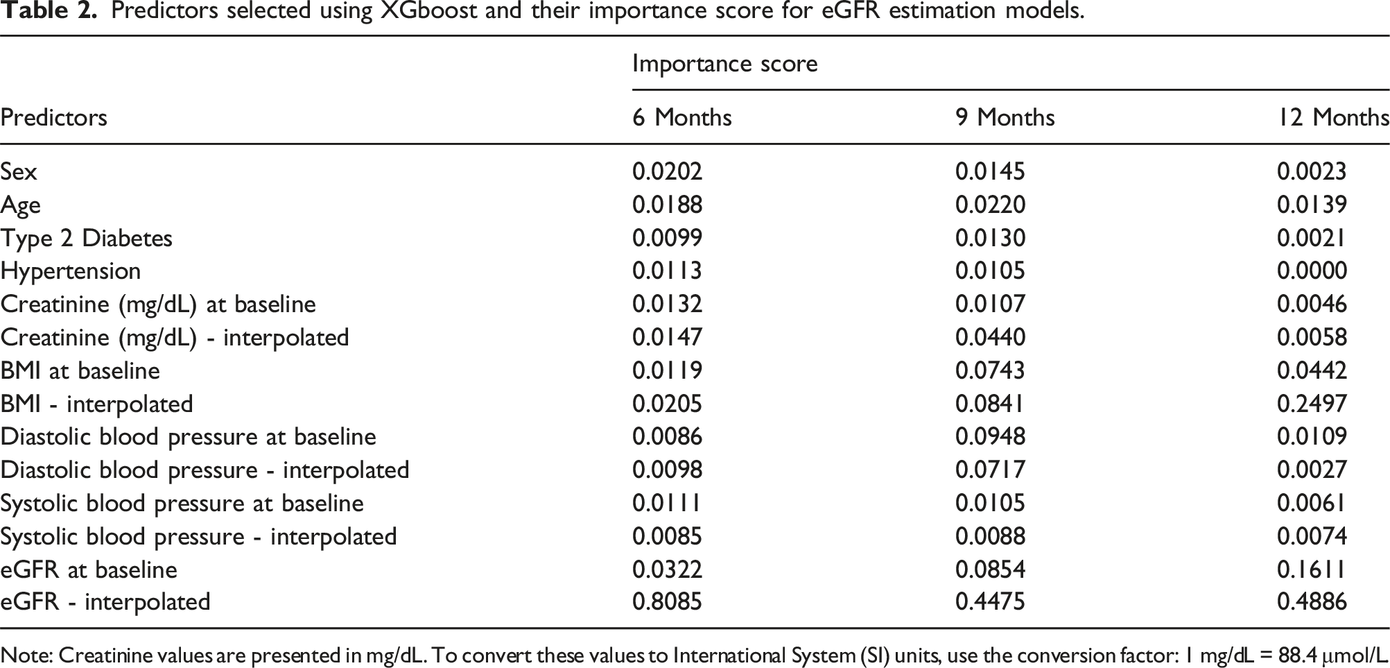
Note: Creatinine values are presented in mg/dL. To convert these values to International System (SI) units, use the conversion factor: 1 mg/dL = 88.4 μmol/L.

As regards global interpretability, SHAP explains the outcome of a model as the sum of each contributing variable. For our models, greater than zero means that the variable in the present value increases the predicted eGFR, while less than zero indicates the opposite. Figure 2 shows the global feature contribution for each model. In that figure, are shown the features that help drive the model output from the base value (the average model output over the training data set) to the model output. Features that push the highest prediction are shown in red, those that push the lowest prediction are in blue.

Figure 2.

Beeswarm plot where each point corresponds to an individual patient in the study. Dot position on the x-axis shows the impact that characteristic has on the model’s prediction for that patient. When several dots fall on the same x-position, they accumulate to show the density. (a) 6-months prediction model; (b) 9-months prediction model, (c) 12-months prediction model.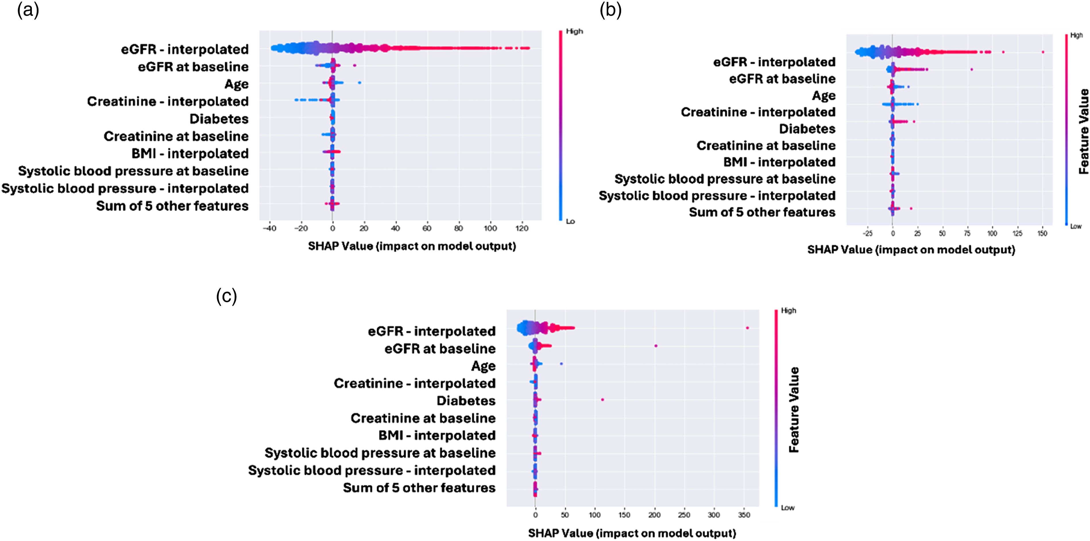

For all prediction models, the most contributing variables were eGFR– interpolated, eGFR at baseline, age, and creatinine– interpolated with lower values (below zero) indicating lower predicted eGFR values. Furthermore, only for the 6-month prediction model, type 2 diabetes was in the top 5 of the predictors with the highest contributions.

It is interesting to note that interpolated variables were the most important features, pointing out the relevance of the longitudinal treatment of the variables in ML models.

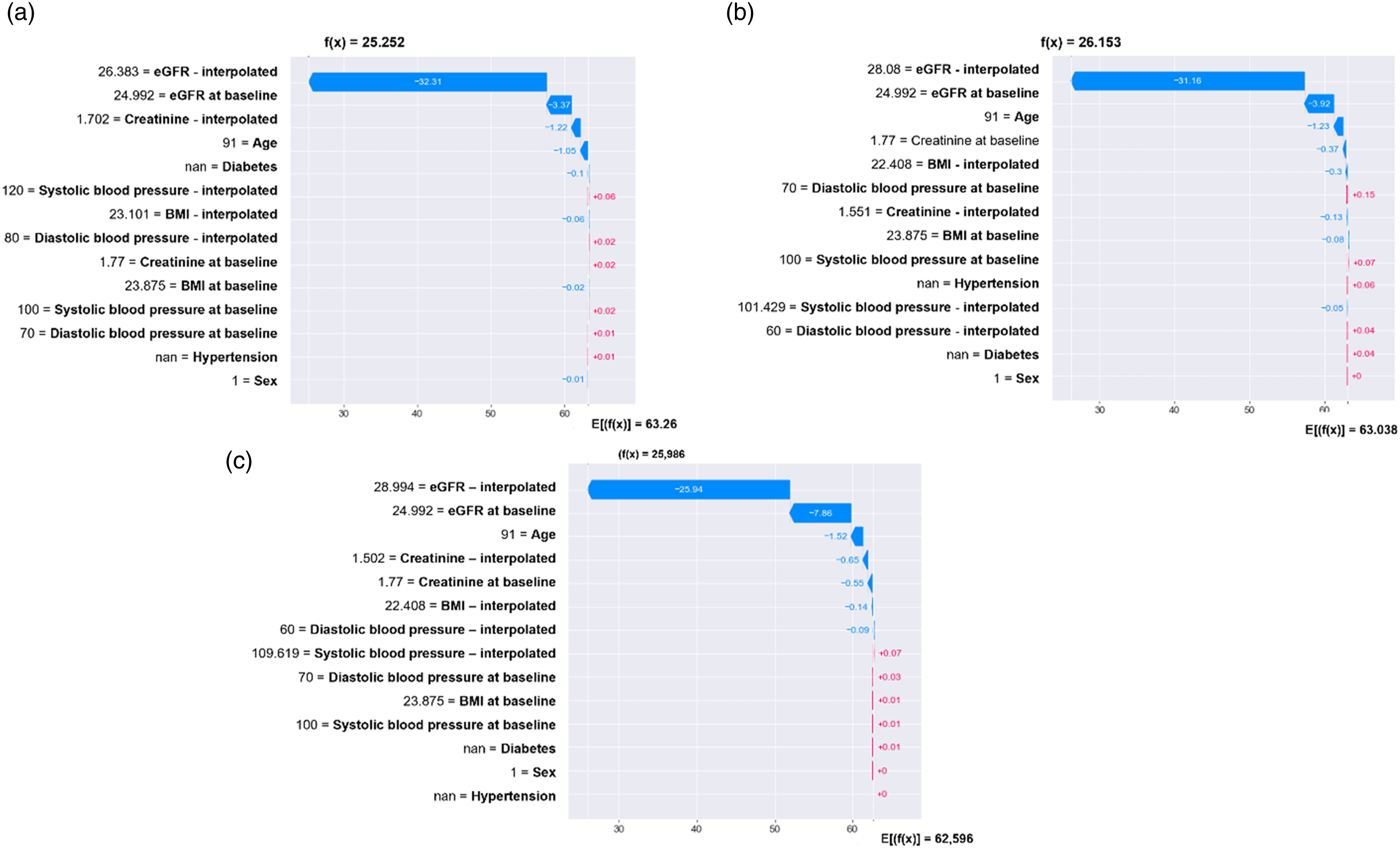
Figures 3 and 4 show the use of SHAP for local interpretability aimed to know the attribution of each variable in terms of its weight indicated as the length of the bar and direction force towards the outcome score (positive or negative). Besides, f(x) indicates the predicted eGFR value for that individual patient, while E[f(X)] indicates the average predicted eGFR for the entire cohort.

Figure 3.

Waterfall plot for a single patient. The contributing variables are arranged in the x-position, sorted by the absolute value of their impact. Variables in the red arrow mean the impact values are positive while blue means negative. (a) The predicted eGFR value at 6-months is 62.88. eGFR – interpolated 65.59, creatinine (mg/dL) – interpolated 1.23, and SBP at baseline 150 were the main factors that pushed the predicted eGFR value to lower values. eGFR at baseline 70.63, age 51, not having diabetes diagnosis, and creatinine at baseline 1.05 were the main factors that pushed the predicted eGFR value to higher values. (b) The predicted eGFR value at 9-months. (c) The predicted eGFR value at 12-months.

Figure 4.

Waterfall plot for a single patient. (a) The predicted eGFR value at 6 months is 25.25. eGFR – interpolated 26.38, eGFR at baseline 24.99, creatinine (mg/dL) interpolated 1.70, and age 91 were the main factors that pushed the predicted eGFR value to lower values. Almost no other variable pushed the predicted eGFR value to higher values. (b) The predicted eGFR value at 9-months. (c) The predicted eGFR value at 12-months.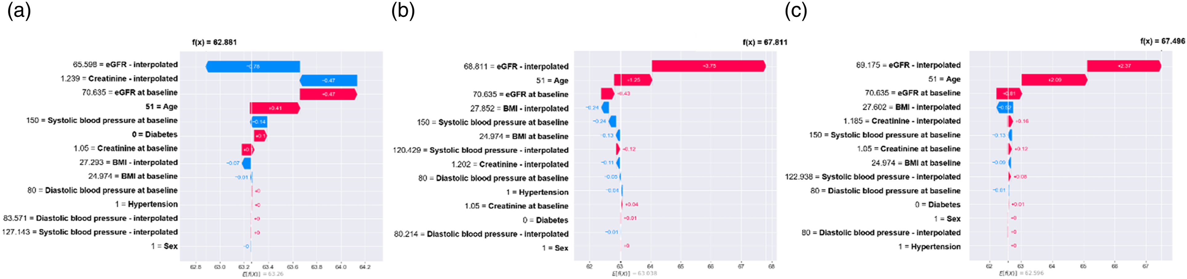

Discussion

In this study, we developed three machine learning models to predict the next eGFR at different intervals. We used few and commonly captured variables, even for resource-constraint environments. MAE values showed that all predictive models had a good performance, and they can be implemented as a useful early warning system for screening and identification of patients at high risk of CKD progression.

Our models have an additional advantage over most other predictive models for CKD, they are not black-boxes, and their interpretation is available for clinicians. The aforementioned is a highly relevant factor since healthcare professionals need interpretable and transparent information to support the intervention they will perform according to the risk level identified in the patient.^19,20

Decision-makers in healthcare have pointed out the interpretability of model predictions as a priority for implementation and utilization.²¹ Hence, in the current study we considered two aspects: (1) ML models described in this study are designed to assist healthcare professionals across clinical care and costs domains; (2) decisions based on predictions will inform clinical care pathways, patient risk stratification, and possibly many others.

To the best of our knowledge, there are few published reports about predictive models that have attempted to predict the next eGFR. Besides, none have captured clinical and laboratory variables commonly collected in care models for chronically ill patients in low- and middle-income countries. For instance, although with excellent performance some of them have included laboratory variables such as serum calcium, bicarbonate, and phosphorous which are not collected for the entire at-risk CKD population in Colombia.²²

On the other hand, we implemented a method to handle and take advantage of longitudinal data. Recently, a group of evidence has emphasized the need to overcome using cross-sectional data for predictive models as an essential forward-step for public health.^23,24 Studies using large population samples with data extracted from electronic health records showed that models developed with transformed longitudinal data outperformed the traditional predictive models used clinically.^25–27

Likewise, our study is the first one that attempted to predict eGFR using transformed clinical longitudinal data into interpretable ML models. Besides, to our knowledge, this is the first study that includes such a large South American sample of CKD patients to develop predictive models. The models’ performance was good in external validation cohorts and with similar performance to previously developed predictive models.²⁸

In this study, we selected the XGBoost (Extreme Gradient Boosting) algorithm for predicting the next eGFR due to its superior performance in handling complex datasets and its effectiveness in capturing non-linear relationships. XGBoost is a gradient boosting framework that is renowned for its efficiency, scalability, and accuracy in predictive modeling.²⁹ It combines several boosting techniques to create a powerful model that can handle large datasets with high dimensionality, making it particularly suitable for our prediction tasks.

XGBoost has been widely recognized in the literature for its high accuracy and performance across various machine learning challenges, including regression tasks similar to our study.³⁰ Its ability to improve model performance through boosting and regularization techniques ensures accurate predictions. Furthermore, the algorithm’s capacity to model complex, non-linear interactions between features allows it to effectively capture intricate patterns in the data, which is crucial for predicting eGFR with a high degree of precision. Lastly, XGBoost provides insights into feature importance, which helps in understanding the contribution of different variables to the prediction outcome.³¹ This interpretability is valuable for clinical applications where understanding the impact of various factors on eGFR is essential.

The findings of the present study support the use of ML models to identify CKD patients at higher risk for accelerated CKD progression who may benefit from effective preventive strategies. Furthermore, our predictive models have been recently implemented on a care model for chronically ill Colombian patients through an application programming interface. The next step will be to evaluate the cost-effectiveness and clinical utility of these models in real-world practice.

Our study has some limitations. First, the impossibility to include a geographically different population from that of the Colombian Caribbean region to assess models’ external validity. In addition, laboratory variables such as albuminuria, glycosylated hemoglobin, total cholesterol, and high-density lipoprotein cholesterol were not included due to a large amount of missing data. As well as relevant sociodemographic variables such as household monthly income and education level were also not included.

The above is pertinent since those variables could be relevant predictors for CKD progression in our population.^32,33 Nevertheless, through the use in real-world practice, ML models can be continuously updated as these data become available in additional cohorts.

Lastly, an additional significant limitation was the absence of medication data within the dataset. Medications can profoundly affect kidney function and progression, and their exclusion from our analysis means we could not account for these potential influences on GFR predictions. Future research should aim to include detailed medication information to better assess its effects on GFR and improve predictive accuracy.^34,35

Conclusions

Our study developed and validated machine learning models to predict eGFR at 6, 9, and 12-month intervals, demonstrating good performance across both internal and external validation cohorts. The 6-month prediction model showed the best overall performance. Key predictors included interpolated eGFR values and baseline measurements, which proved crucial for accurate forecasts. The models’ interpretability, enabled by SHAP values, enhances their clinical relevance by offering insights into how individual variables influence eGFR predictions. Despite some limitations, such as missing data on certain laboratory variables and medication information, our models provide a valuable tool for early risk identification and intervention in CKD management. The interpretability of the prediction results can offer deeper insight into the changes in eGFR induced by specific variables, hence could support the decision-makers in healthcare and clinicians for early intervention of the modifiable factors.

Future studies should incorporate additional data to further refine these predictions and assess their real-world utility and cost-effectiveness.

Footnotes

Acknowledgements

The authors would like to thank Asociación Colombiana de Nefrología e Hipertensión Arterial for their discussions.

Declaration of conflicting interests

The author(s) declared no potential conflicts of interest with respect to the research, authorship, and/or publication of this article.

Funding

The author(s) disclosed receipt of the following financial support for the research, authorship, and/or publication of this article: This work was supported by the Science for Life (S4L).

Ethical approval

Guarantor

LHR.

Contributorship

LHR, AM, and AJPM conceived the study. LHR, WA and AM were involved in protocol development and data analysis. WA was involved in database management and data analysis. VD and WV were involved in databases building and reviewing results. AJPM wrote the first draft of the manuscript. All authors reviewed and edited the manuscript and approved the final version.

Data availability statement

The authors reserve data and code availability due to the existence of a confidentiality agreement with the health care provider who shared their data for the study. Furthermore, the models described, and data sets included are currently part of an ongoing research project to implement a risk stratification system in clinical practice.

ORCID iD

Luis H Rojas

References

Bikbov

Purcell

Levey

, et al. Global, regional, and national burden of chronic kidney disease, 1990–2017: a systematic analysis for the Global Burden of Disease Study 2017. Lancet 2020; 395(10225): 709–733. https://linkinghub.elsevier.com/retrieve/pii/S0140673620300453

Coresh

. Update on the burden of CKD. J Am Soc Nephrol 2017; 28(4): 1020–1022. https://jasn.asnjournals.org/lookup/doi/10.1681/ASN.2016121374

Stanifer

Von

Chertow

, et al. Chronic kidney disease care models in low- and middle-income countries: a systematic review. BMJ Glob Heal 2018; 3(2): e000728. https://gh.bmj.com/content/3/2/e000728

Hosseinpoor

Bergen

Kunst

, et al. Socioeconomic inequalities in risk factors for non communicable diseases in low-income and middle-income countries: results from the World Health Survey. BMC Publ Health 2012; 12: 912. https://pubmed.ncbi.nlm.nih.gov/23102008/

Luyckx

Tonelli

Stanifer

. The global burden of kidney disease and the sustainable development goals. Bull World Health Organ 2018; 96(6): 414–422D.

Tonelli

Dickinson

. Early detection of CKD: Implications for low-income, middle-income, and high-income countries. J Am Soc Nephrol. 2020; 31(9):1931–1940. https://jasn.asnjournals.org/content/31/9/1931

Ali

Kalra

. Risk prediction in chronic kidney disease. Curr Opin Nephrol Hypertens 2019; 28(6): 513–518. https://journals.lww.com/00041552-201911000-00003

Beam

Kohane

. Big data and machine learning in health care. JAMA 2018; 319(13): 1317–1318. https://jama.jamanetwork.com/article.aspx?doi=10.1001/jama.2017.18391

Smiti

. When machine learning meets medical world: current status and future challenges. Comput Sci Rev 2020; 37: 100280. https://linkinghub.elsevier.com/retrieve/pii/S157401372030126X

10.

Wainstein

Bello

Jha

, et al. International Society of nephrology global kidney health atlas: structures, organization, and services for the management of kidney failure in Latin America. Kidney Int Suppl 2021; 11(2): e35–46. https://linkinghub.elsevier.com/retrieve/pii/S2157171621000125

11.

Sarmiento-Bejarano

Ramírez-Ramírez

Carrasquilla-Sotomayor

, et al. Carga económica de la enfermedad renal crónica en Colombia, 2015-2016. Vol. 35, Revista Salud Uninorte. scieloco; 2019. p. 84–100.

12.

Rivera-Caravaca

Ruiz-Nodar

Tello-Montoliu

, et al. Disparities in the estimation of glomerular filtration rate according to cockcroft-gault, modification of diet in renal disease-4, and chronic kidney disease epidemiology collaboration equations and relation with outcomes in patients with acute coronary. J Am Heart Assoc. 2018; 7: e008725.

13.

Chen

Guestrin

. XGBoost: a scalable tree boosting system, 2016. https://arxiv.org/abs/1603.02754

14.

Lundberg

Lee

S-I

. A unified approach to interpreting model predictions. Adv Neural Inf Process Syst. 2017; 30: 4768–4777.

15.

Bowen

Ungar

. Generalized SHAP: generating multiple types of explanations in machine learning, 2020. https://arxiv.org/abs/2006.07155

16.

Lundberg

Erion

Chen

, et al. From local explanations to global understanding with explainable AI for trees. Nat Mach Intell 2020; 2(1): 56–67. https://www.nature.com/articles/s42256-019-0138-9

17.

Martinez

Soto

Eraso

, et al. Towards guidelines for management and custody of electronic health records in Colombia, 2017, pp. 749–758. https://link.springer.com/10.1007/978-3-319-66562-7_53

18.

Cabitza

Campagner

. The need to separate the wheat from the chaff in medical informatics: introducing a comprehensive checklist for the (self)-assessment of medical AI studies. Int J Med Inform 2021; 153: 104510. https://linkinghub.elsevier.com/retrieve/pii/S1386505621001362

19.

Vellido

. The importance of interpretability and visualization in machine learning for applications in medicine and health care. Neural Comput Appl 2020; 32(24): 18069–18083. https://link.springer.com/10.1007/s00521-019-04051-w

20.

Katuwal

Chen

. Machine learning model interpretability for precision medicine, 2016. https://arxiv.org/abs/1610.09045

21.

Ahmad

Eckert

Teredesai

. Interpretable machine learning in healthcare. In: Proceedings of the 2018 ACM International Conference on Bioinformatics, Computational Biology, and Health Informatics, New York, NY, USA, 2018, pp. 559–560. ACM. https://dl.acm.org/doi/10.1145/3233547.3233667

22.

Futoma

Sendak

Cameron

, et al. Predicting disease progression with a model for multivariate longitudinal clinical data. In: Machine Learning for Healthcare Conference, 2016, pp. 42–54. PMLR.

23.

Vidal-Petiot

Stebbins

Chiswell

, et al. Visit-to-visit variability of blood pressure and cardiovascular outcomes in patients with stable coronary heart disease. Insights from the STABILITY trial. Eur Heart J 2017; 38(37): 2813–2822. https://academic.oup.com/eurheartj/article/38/37/2813/3852229

24.

Ravizza

Huschto

Adamov

, et al. Predicting the early risk of chronic kidney disease in patients with diabetes using real-world data. Nat Med 2019; 25(1): 57–59. https://www.nature.com/articles/s41591-018-0239-8

25.

Zhao

Feng

, et al. Learning from longitudinal data in electronic health record and genetic data to improve cardiovascular event prediction. Sci Rep 2019; 9(1): 717. https://www.nature.com/articles/s41598-018-36745-x

26.

Wong

Y-K

Chan

Y-H

Hai

JSH

, et al. Predictive value of visit-to-visit blood pressure variability for cardiovascular events in patients with coronary artery disease with and without diabetes mellitus. Cardiovasc Diabetol 2021; 20(1): 88. https://cardiab.biomedcentral.com/articles/10.1186/s12933-021-01280-z

27.

Low

Zhang

Ang

, et al. Discovery and validation of serum creatinine variability as novel biomarker for predicting onset of albuminuria in Type 2 diabetes mellitus. Diabetes Res Clin Pract 2018; 138: 8–15. https://linkinghub.elsevier.com/retrieve/pii/S016882271731392X

28.

Norouzi

Yadollahpour

Mirbagheri

, et al. Predicting renal failure progression in chronic kidney disease using integrated intelligent fuzzy expert system. Comput Math Methods Med 2016; 2016: 6080814–6080819. https://www.hindawi.com/journals/cmmm/2016/6080814/

29.

Arif Ali

H Abduljabbar

A Tahir

, et al. eXtreme gradient boosting algorithm with machine learning: a review. Acad J Nawroz Univ 2023; 12(2): 320–334. https://journals.nawroz.edu.krd/index.php/ajnu/article/view/1612

30.

Zhang

Yuan

Yao

, et al. Improvement of the performance of models for predicting coronary artery disease based on XGBoost algorithm and feature processing technology. Electronics 2022; 11(3): 315. https://www.mdpi.com/2079-9292/11/3/315

31.

Meng

Yang

Qian

, et al. What makes an online review more helpful: an interpretation framework using XGBoost and SHAP values. J Theor Appl Electron Commer Res 2020; 16(3): 466–490. https://www.mdpi.com/0718-1876/16/3/29

32.

Huda

Alam

Ur-Rashid

. Prevalence of chronic kidney disease and its association with risk factors in disadvantageous population. Int J Nephrol 2012; 2012: 1–7. https://www.hindawi.com/journals/ijn/2012/267329/

33.

Vesga

Cepeda

Pardo

, et al. Chronic kidney disease progression and transition probabilities in a large preventive cohort in Colombia. Int J Nephrol. 2021; 2021: 1–9. https://www.hindawi.com/journals/ijn/2021/8866446/

34.

Verdalles

Goicoechea

Garcia de Vinuesa

, et al. Prevalence and characteristics of patients with resistant hypertension and chronic kidney disease. Nefrologia 2016; 36(5): 523–529. https://www.ncbi.nlm.nih.gov/pubmed/27445099

35.

Norris

Williams

Nicholas

, et al. Current view on CKD risk factors: traditional, noncommunicable diseases—diabetes, hypertension, and obesity. In: Chronic Kidney Disease in Disadvantaged Populations. Amsterdam: Elsevier, 2017, pp. 183–190. https://linkinghub.elsevier.com/retrieve/pii/B9780128043110000194

Development and validation of interpretable machine learning models to predict glomerular filtration rate in chronic kidney disease Colombian patients

Abstract

Background

Objective

Study Design and Setting

Results

Conclusion

Keywords

Introduction

Methods

Population - study cohorts

Outcome

Candidate predictors

Estimating values for prediction intervals

Internal and external validation samples

Models developing

Internal and external validation

Interpretability of models

Results

Discussion

Conclusions

Footnotes

Acknowledgements

Declaration of conflicting interests

Funding

Ethical approval

Guarantor

Contributorship

Data availability statement

ORCID iD

References