Sage Journals: Discover world-class research

Abstract

Background

Risk management strategies have been proposed for applications in clinical laboratories to reduce patient risks; however, effective and visual risk-monitoring tools are currently lacking in medical laboratories. In this study, we constructed a risk quality control (QC) chart based on risk management strategies.

Methods

We calculated the risk levels of QC materials based on Bayes' theorem by combining the total allowable error, QC results, and the maximum number of unacceptable errors in the laboratory. Then, we constructed a risk QC chart by presenting the Z values and corresponding risk levels of QC materials simultaneously. Finally, we evaluated the risk-monitoring capabilities of the risk QC charts by simulating different long-term errors in the laboratory.

Results

The risk levels of QC materials increased as the QC results moved further away from the set mean. Larger sigma values led to fewer risks obtained for the same QC results. The constructed risk QC charts intuitively showed specific risk levels and could warn lab staff out-of-control, without the need for QC rules to make judgments. The risk levels of erroneous results differed for items with different sigma performance.

Conclusions

Risk-based QC charts allowed visualization of the QC results and specific risk levels simultaneously, providing more intuitive results than those obtained from traditional QC charts.

Keywords

Quality control risk management risk quality control chart

Introduction

Quality control (QC) in medical laboratories has greatly advanced. In 1950, Levey and Jennings¹ introduced Shewhart QC charts for use in industrial manufacturing² to the clinical chemistry field to monitor product quality by detecting trends in QC data measured daily. These QC charts were named the “Shewhart QC charts” or “Levey–Jennings (L-J) QC charts.” In 1952, Henry and Segalove³ developed an alternative method in which fresh samples were randomly mixed and repeatedly measured, and individual QC results were plotted on L-J QC charts. In 1959, Henry⁴ described the application of the 1s, 2s, and 3s rules in the L-J QC charts. In 1977, Westgard et al.⁵ proposed multi-rule QC methods based on Henry rules (adding 2-2s, 4-1s, R-4s, and 10x). Westgard et al.⁶ also recommended establishing QC procedures based on the sigma metrics of the test items. Greater sigma values led to better performance of the detection systems, whereas smaller sigma values led to worse performance. Therefore, sigma metrics are essentially based on risk management.⁶

In 2008, Parvin⁷ proposed a risk surrogate index MaxE(N_uf), defined as the expected number of unreliable patient results generated and reported before the out-of-control condition was detected. In 2011, the Clinical and Laboratory Standards Institute (CLSI) published Guideline EP23-A: “Risk Management-Based Laboratory Quality Control Guide”⁸ and fourth edition of Guideline C24: “Quantitative Measurement Program Statistical Quality Control: Principles and Definitions” in 2016.⁹ These two guidelines outlined new requirements for QC based on risk management, marking the transition of the focus of statistical quality control (SQC) from the stability of the analytical systems (centered around analytical instruments) to patient risks in the laboratory.

In the context of risk management-based QC systems, Yago and Alcover^10,11 and Bayat¹² combined the classical Westgard QC method with the Parvin risk management strategy to improve SQC and reduce patient risks. This risk-based QC system described the association between the probability of error detection (P_ed) and MaxE(N_uf); that is, a detection system with a high P_ed had a low MaxE(N_uf). Westgard et al.¹³ further mapped the relationship between P_ed and MaxE(N_uf) into a nomogram to estimate the analytical batch size (QC frequency) using the following formula: QC frequency = 100/MaxE(N_uf). By combining risk management and SQC data, this nomogram guided laboratories to establish QC plans to achieve the risk target of MaxE(N_uf) ≤1 and ensure that the number of unreliable patient results reported met QC requirements.

Despite great progress in QC management in medical laboratories, L-J QC charts remain widely used, no longer meeting the current QC requirements of risk management.¹⁴ L-J QC charts were based on the traditional SQC, relying on QC rules to determine whether it was out-of-control. However, L-J QC charts cannot reflect specific risk levels, and effective and visual risk-monitoring tools are currently lacking. Therefore, this study was conducted to establish a novel risk-based QC chart to visualize the risk levels of QC materials in clinical laboratories.

Materials and methods

Parameters of risk quality control charts

We constructed risk QC charts according to the following parameters: total allowable error (TEa), which was based on the People’s Republic of China Health Industry Standard (WS/T 403–2012)¹⁵; bias, which was derived from the results of external quality assessment of the Ministry of Health; and risk management control limit (RMCL), which was the acceptable MaxE(N_uf) for analytical batch and was set by the laboratory staff.⁷

Calculating risk levels based on Bayes' theorem

Conventionally, QC results were visualized using L-J QC charts, and the out-of-control status was judged according to the Westgard QC rules.¹⁶ In this study, we calculated the risk levels of QC materials according to Bayes' theorem¹⁷ and visualized the risk levels in the risk QC charts. Risks were defined as the probability that the QC results exceeded the TEa. The detailed calculation steps were as follows.

(1) QC results without out-of-control

First, we assumed that QC result A was not out-of-control and conformed to a normal distribution with a mean of u and standard deviation (SD) of sd, which was represented by N(u, sd). The probability distribution of results on an in-control QC specimen was P(A) [N(u, sd)].

(2) QC results with out-of-control

Next, we assumed that QC result B was out-of-control and conformed to a normal distribution with a mean of u_o and SD of sd_o. Subscript “O” indicated out-of-control. The probability distribution of the out-of-control QC specimen was P(B) [N (u_o, sd_o)].

(3) QC results with random situations

According to the probability theory, the probability distribution of QC results with random situations in the laboratory was calculated as P(A|B), which was the probability of the mean at a certain position when the QC results were out-of-control.

(4) Probability distribution of risk levels

P(B|A) was the probability distribution of risk levels, that was the probability of out-of-control for in-control QC specimen. According to Bayes' theorem,¹⁷ the statistical parameter was calculated as P(B|A) = P (A|B) × P(B)/P(A).

Specific formulas for calculating the risk levels

The specific formulas used to calculate the risk levels of QC materials were as follows.

(1) The distribution of the detection system was calculated:

u_{t} = \frac{s d_{0}^{2} \times \sum x + s d^{2} \times u_{o}}{n_{r} \times s d_{0}^{2} + s d^{2}}, s d_{t} = \sqrt{\frac{s d^{2} \times s d_{0}^{2}}{(n_{r} \times s d_{0}^{2} + s d^{2})}}

(1)

u_{t}, s d_{t}

represent the mean and SD of the detection system; u and sd were the mean and SD of QC materials without out-of-control, u_o and sd_o were the mean and SD of QC materials with out-of-control, x was the result of each QC, and n_r was the number of repetitions of the QC materials.

(2) When a systematic error (SE) occurred, the probability (P_X) was calculated based on the normal distribution:

P_{X} = Ø (s e + d x, u_{t}, s d_{t}) - Ø (s e, u_{t}, s d_{t})

(2)

where Ø was the area under the standard normal distribution curve

Ø (x) = \frac{1}{\sqrt{2 π}} \int_{- \infty}^{x} e^{- t^{2} / 2} d t

(3)

se was the systematic error generated in the analysis; dx was the differentiation; u_t and sd_t were the mean and SD of the detection system.

(3) When QC results exceeded TEa, the probability (P_TEa) was calculated:

P_{T E a} = Ø (u - T E a, s e, s d) + 1 - Ø (u + T E a, s e, s d)

(4)

TEa was the total allowable error, se was the systematic error, and u and sd were the mean and SD of QC materials without out-of-control.

(4) The probability of unacceptable results at a certain SE $(P_{s e_x})$ was calculated:

P_{s e_x} = P_{X} \times P_{T E a}

(5)

That was the probability of exceeding the TEa when SE occurred.

(5) The risk levels of QC materials were calculated:

Risk levels $(P_{s e})$ were the probability of unacceptable results with different SE and was calculated by integrating $P_{s e_x}$ in different situations.

P_{s e} = \int_{- \infty}^{\infty} P_{s e_x} d s e

(6)

For the detailed calculation methods and formula derivation, please refer to patent CN110135731 A (Google Patent Search) and Supplemental Materials.

Constructing novel risk quality control charts

After calculating the risk levels of QC materials, we analyzed the traditional Z values of the QC results (Z = (x-u)/sd). x was each QC result, u and sd were the mean and SD of accumulated QC results. Then, we constructed a novel risk QC chart by simultaneously presenting the Z values and corresponding risk levels as vertical coordinates. The Z values were visualized using line charts, and the risk levels were visualized using bar graphs. The days (dates) of QC events were used as horizontal coordinates. The RMCL was drawn parallel to the horizontal coordinates to monitor the risk levels intuitively. In our study, the RMCL was set to 0.01 (1%) based on general inspection.⁷ When the risk levels exceeded the RMCL, an alarm would be triggered.

Simulating different long-term errors in medical laboratories

To investigate the risk-monitoring capabilities of the risk QC charts, we simulated different long-term errors in medical laboratories. The QC results of total protein (TP) for 30 consecutive days were selected for the case simulation. There were two levels of QC material: QC level 1: u = 39.60 g/L, sd = 0.56 and QC level 2: u = 69.10 g/L, sd = 0.88, TEa = 6%.

First, we calculated the probability distribution of SE (P_x)and exceeded TEa ( $P_{T E a})$ . Next, we calculated the risk levels $(P_{s e})$ for QC results with different biases. We also observed the trends in risk levels for QC results with different sigma values. Finally, we simulated different laboratories with different long-term errors. Briefly, we assumed that five laboratories (labs A–E) had different out-of-control frequencies compared to our laboratory. Among them, lab A and lab B had the same sigma performance as our lab, but lab A was more frequently out-of-control and lab B was less out-of-control. Lab C, Lab D, and Lab E had higher sigma performance (7-sigma: u = 69.10 g/L, sd = 0.60), while Lab C was less often out-of-control, Lab D the same out-of-control, and Lab E more often out-of-control than our lab.

Our medical laboratory is in a large 3A grade hospital and operates according to standard operating procedures, performs internal quality control of two levels of QC materials every day, and participates in annual external quality evaluation by the Ministry of Health. In addition, our laboratory is accredited by the College of American Pathologists, indicating that our results are relatively accurate and reliable and meet the requirements of quality specifications.

All simulations and analyses were performed using Python 3.7 (Numpy and Scipy packages). Microsoft Excel 2016 was used to draw and design tables. The raw data and codes were provided in the Supplemental Material.

Results

Probability distributions of SE and exceeding TEa

According to formulas (1)–(4), we first calculated the probability distributions of the SE and exceeded the TEa. Interestingly, the probability for SE satisfied a normal distribution and concentrated on a value that was close to the mean of the QC results. A larger number of QC repetitions led to a more concentrated distribution, and vice versa. QC level 2 was used as an example; the distribution of SE was normally distributed with a mean value near 69.10 g/L (mean = 69.03 g/L), with the probability increased from a concentration close to 69.10 g/L and probability decreased away from this value. However, the probability distributions exceeding TEa exhibited a concave curve distribution. When SE was 0 (mean = 69.10 g/L), the probability of exceeding the TEa was minimal; as SE increased, the probability of exceeding the TEa also increased and converged to 1 (Figure 1).

Figure 1.

Probability distributions of systematic errors and exceeding the total allowable error (TEa). The X-axis is the difference in quality control results and set mean 69.10 g/L. The Y-axis is the probability distribution of systematic error and exceeds the TEa.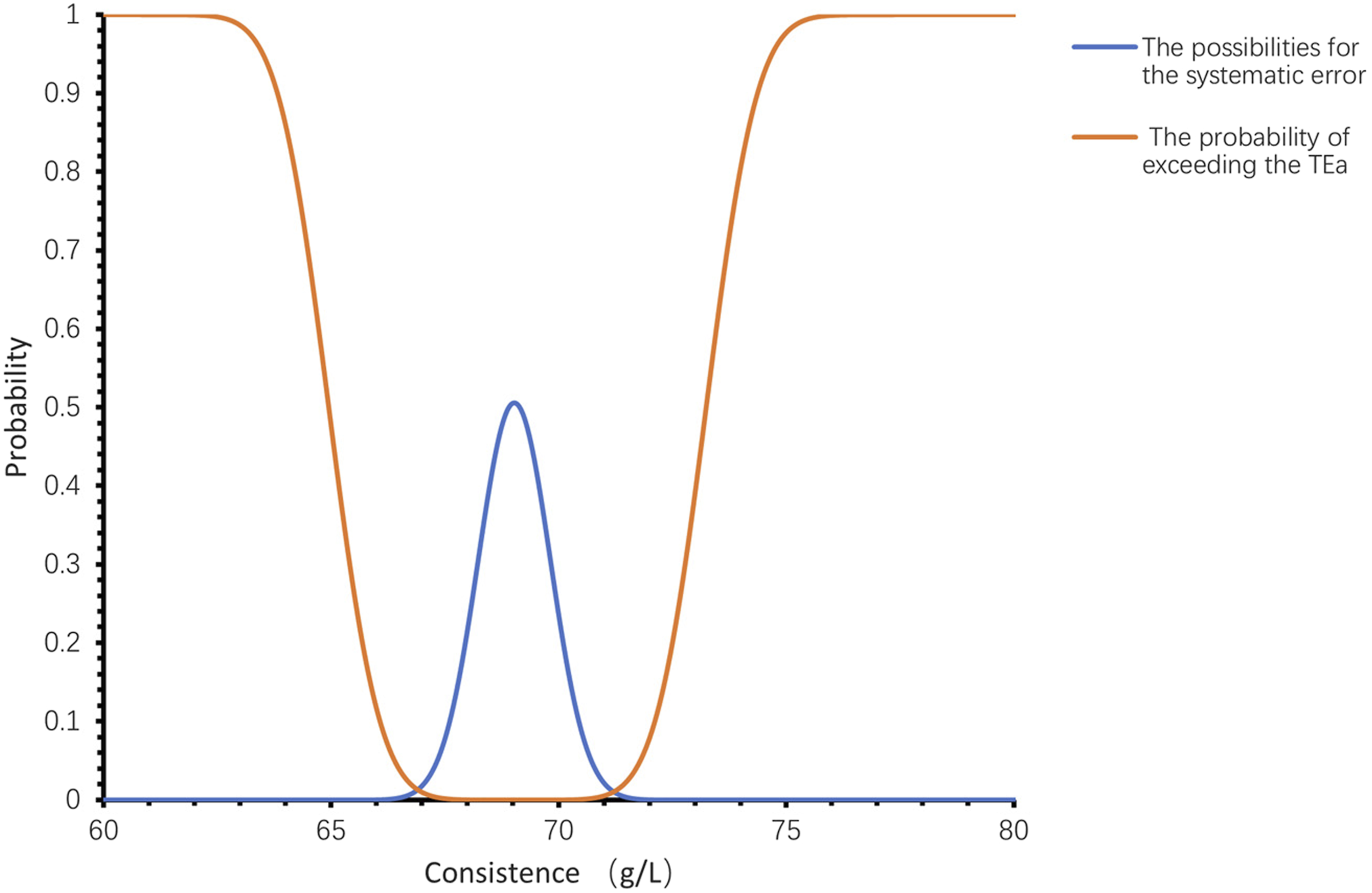

Probability distributions of risk levels

We calculated the probability distributions of the risk levels with different biases according to Equations (5) and (6). As shown in Figure 2(a), the risk level was 0.00,028 for QC level 2, which was an acceptable result compared to the set RMCL of 0.01. We observed two peaks for the distributions of risk levels when the probability of SE (centered at 69.10 g/L) was multiplied by the probability of exceeding the TEa (centered at 69.03 g/L).

Figure 2.

Probability distributions of risk levels (A); Relationships between Z values and risk levels with different sigma values (B). A: The X-axis is the difference in quality control (QC) results and set mean 69.10 g/L. The Y-axis is the probability distribution of risk levels. B: Z values of QC results were calculated as Z = (x-u)/sd. x represents each QC result, u is the mean of QC materials, and sd is the standard deviation of QC materials. Risk levels refer to the number of test results that exceed the range specified by the total allowable error (TEa).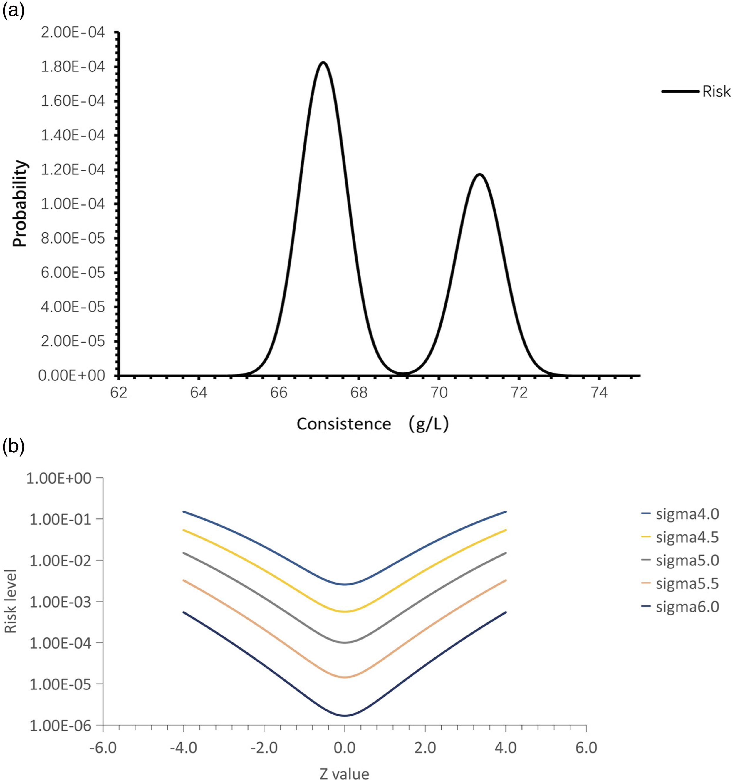

Furthermore, we explored the trends in risk levels for QC results with different sigma values. As shown in Figure 2(b), when simulating the QC data for tests with different sigma performances, different risk levels were obtained for different QC results. As the QC results moved further away from the set mean, the risk levels increased. Larger sigma values led to fewer risk levels obtained for the same QC results.

Visualizing risk levels in risk quality control charts

After calculating the risk levels of QC materials, we visualized the risk levels in the risk QC charts. The mean for QC level 1 was 69.10 g/L and the mean for QC level 2 was 39.60 g/L. The Z values and corresponding risk levels were shown in Figure 3. The yellow line (RMCL) represented the acceptable risk level set by the laboratory staff, and the blue and orange bar graphs represented the probability of unreliable results for the two QC materials. The line charts represented the Z values for the QC results. Using the risk QC chat, we found that the 6th, 10th, 13th, 15th, 23_rd, and 32nd QC results exceeded the RMCL, indicating that there were six batches with TP values exceeding 0.01 (1%), which was the maximum unacceptable risk level. However, using the 6th QC result as an example, out-of-control was not observed based on the Z value. Besides, the last QC level 2 exceeded 3 SD, however, only caused a small risk level.

Figure 3.

Risk quality control charts constructed based on risk management strategies. X-axis: date of quality control (QC) events. Y-axis: Z values (left) and risk levels (right) of QC results. The blue line represents the Z values of QC material 1, and the orange line represents the Z values of QC material 2. The blue and orange bars represent the risk levels of QC materials 1 and 2, respectively. The horizontal yellow line is the risk management control limit (RMCL).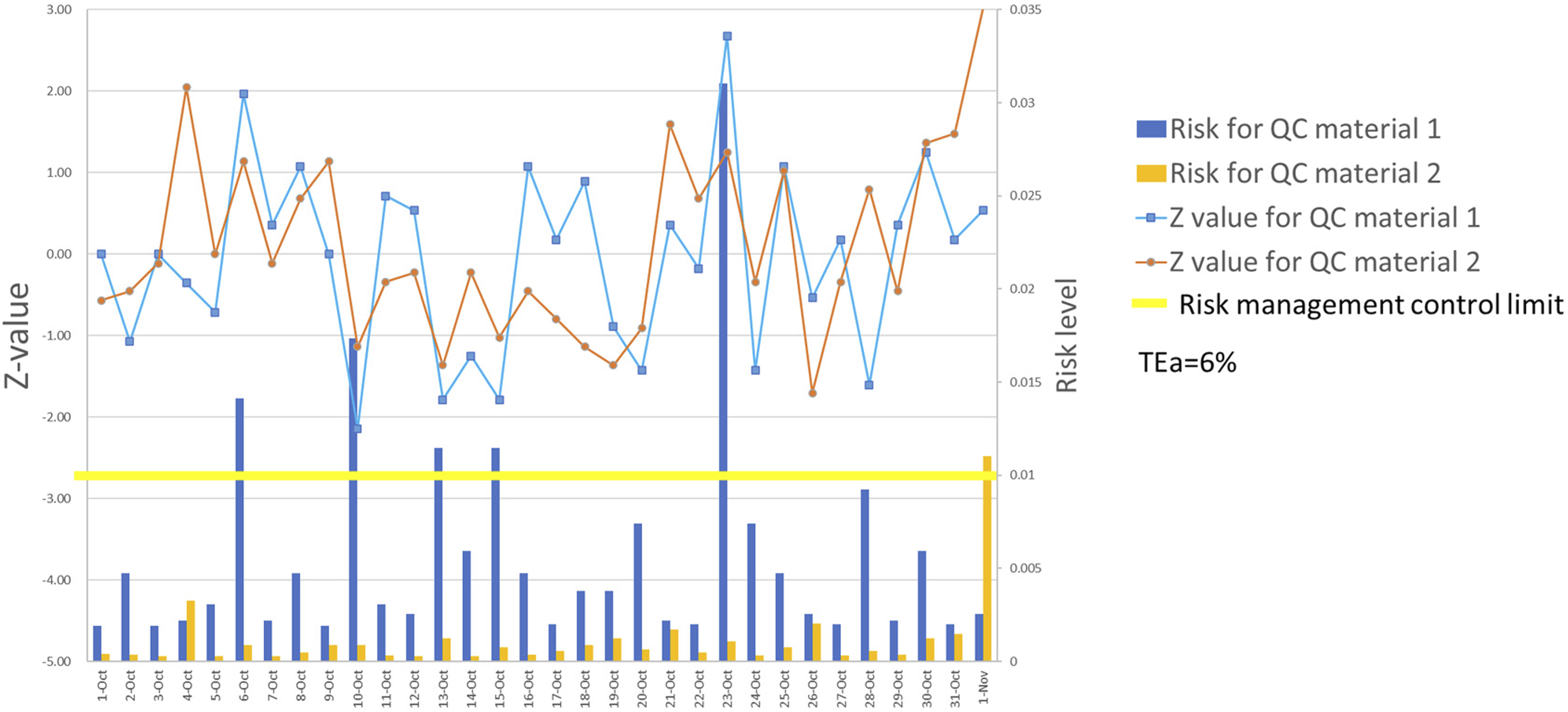

Risk-monitoring capability of risk quality control charts

We investigated the risk-monitoring capabilities of the risk QC charts by simulating different long-term errors in the laboratory. First, the risk QC chart for QC level 2 was constructed according to the actual situation in our laboratory. The QC level consisted of a mean of 69.10 g/L and SD of 0.88. We collected QC results over a period that included data with out-of-control and obtained a long-term mean of 69.20 g/L with an SD of 1.35 (Figure 4(a)).

Figure 4.

Impact of different long-term errors on risk levels of our lab (A), lab A (B), lab B (C), lab C (D), lab D (E), and lab E (F). X-axis: date of quality control (QC) events Y-axis: Z values (left) and risk levels (right) of QC results. The blue line represents the Z values of QC material 2. Orange bars represent the risk levels of QC material 2.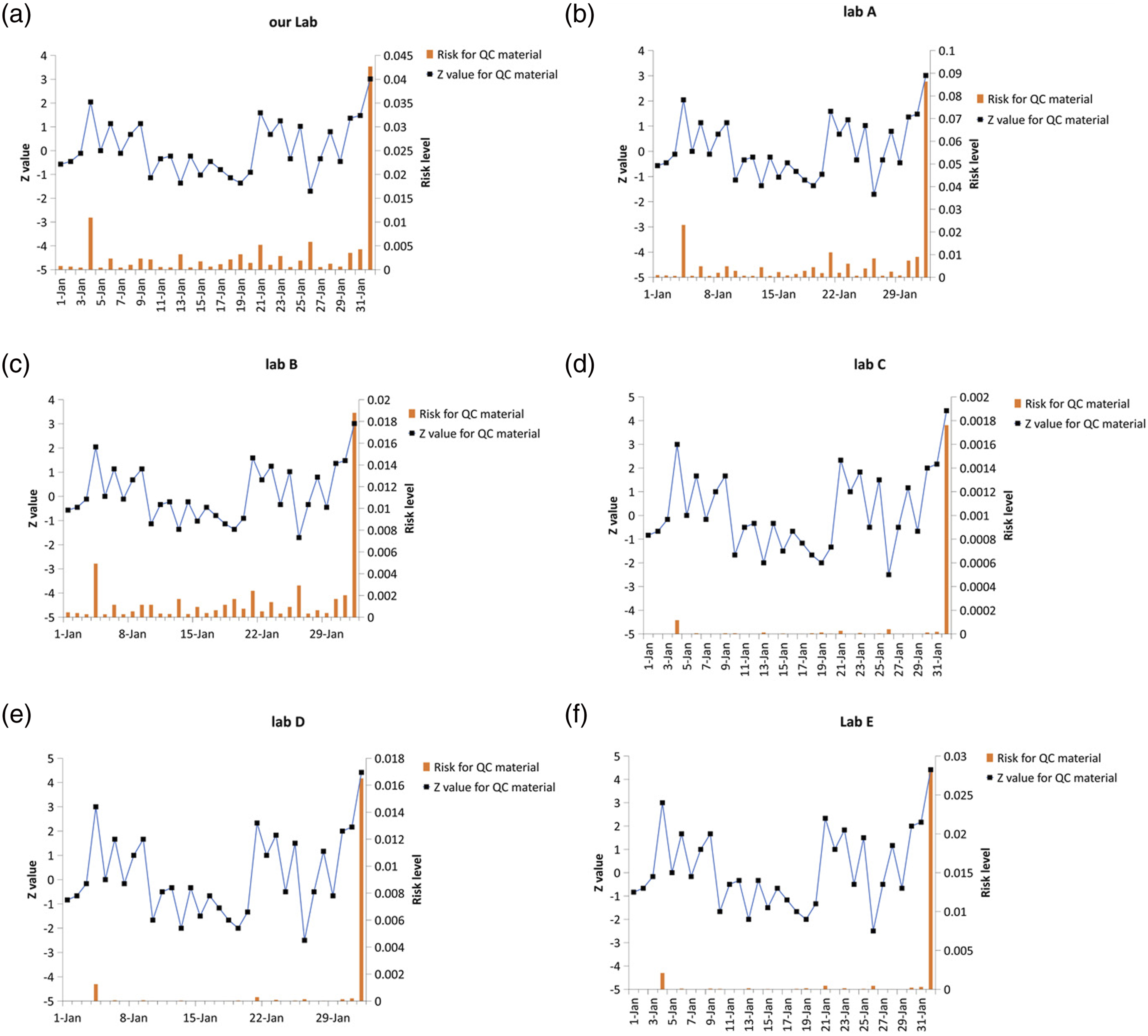

When simulating Lab A, which was out-of-control more often than our lab, we obtained a long-term mean of 70.00 g/L with an SD of 2.35 (Figure 4(b)). However, simulating Lab B, which was out-of-control less often than our lab, had a long-term mean of 69.10 g/L and SD of 0.90 (Figure 4(c)). Lab C with 7-sigma performance had a long-term mean of 69.10 g/L and SD of 0.70 (Figure 4(d)). Lab D was also 7-sigma and out-of-control similar to our lab, with a long-term mean of 69.20 g/L and SD of 1.35 (Figure 4(e)). However, lab E had a long-term mean of 70.00 g/L and SD of 2.35 (Figure 4(f)).

Discussion

Risk management concepts have gradually gained attention in medical laboratories. Traditional SQC rules determine P_ed, which in turn determines the detection capability of laboratory analytical procedures. A higher QC frequency makes it easier to detect analytical errors and reduce patient risks, albeit the laboratory testing cost will increase accordingly. Nevertheless, the positioning of QC has shifted from the reliability of laboratory testing systems to patient risk management. The risk-based QC system can maintain patient risk at an acceptable level by considering patient safety. Although the CLSI C24-Ed4 proposed a QC strategy based on MaxE(N_uf), it did not provide QC charts in actual applications to help laboratories evaluate the risk of the analytical batch. Therefore, we proposed a risk-based QC chart to visually represent the QC results and corresponding risk levels in our study.

Figure 1 showed the probability of different SE and exceeding the TEa. The probability distribution of exceeding the TEa was affected only by the set mean, SD, TEa, and inherent bias; however, the magnitude of SE was influenced by the QC results and was more likely to be close to the mean of QC materials. Figure 2 showed the relationship between the risk levels and Z values with different sigma performances. The Z values represented the difference between the actual QC results and mean and were, therefore, a multiple of the SD¹⁸ Our results indicated that under the same acceptable risk level, a higher sigma performance would have a larger allowable “fluctuation” range of QC results. In contrast, such a range would be narrower for a lower sigma performance.

In this study, the sigma values of the two QC materials for TP were 4.71 and 4.24, respectively. Therefore, when the RMCL was set to 1%, the allowable “fluctuation” range of the QC results was approximate –2SD to 2SD. QC results outside this range might lead to patient risks. However, the Z values and risk levels showed some inconsistencies. The QC results exceeded ±2SD, but the risk levels did not trigger an alert. In addition, the risk levels exceeded 1%, but the Z values were not out-of-control. Therefore, the setting of MaxE(N_uf) is crucial for risk QC charts. To detect projects with low sigma metrics, patient risks could be controlled by adjusting the analytical batch size and acceptable MaxE(N_uf). Taken together, our results showed that the QC scheme was essentially in line with Parvin’s scheme in terms of trends, whereas we explicitly calculated the risk levels. In addition, it was possible to derive Westgard’s scheme from the risk levels, whereas we used a more granular approach. Medical laboratories could combine these two methods (Z values and risk levels) to implement more stringent management of QC results. As for inconsistent alerts, a combination of considerations is needed. Moreover, further research is needed to balance the sensitivity and specificity of combining these two methods.

Currently, clinical laboratories often mitigate patient risks by choosing appropriate QC rules or analytical batch sizes. However, relevant risk-based QC charts are lacking; thus, existing laboratory QC systems could not meet the current risk management requirements. Establishing risk-based QC charts is an important step in achieving risk management in medical laboratories. In this study, risk levels were assessed directly from QC results and performance parameters of analytical instruments to introduce a risk management tool into the laboratory QC system to establish risk-based QC charts.

Using risk QC charts, we clarified the specific risk levels of the analysis batch. In Figure 3, the Z value for the blue line (QC1) on October 22 was lower than the Z value for the orange line (QC2) on November 1; however, the risk level was higher, indicating that QC1 was more likely to become out-of-control than QC2. This information could be communicated to the clinic or patients to inform them of the possible risks of the assay results. Prompted by this risk magnitude, we further investigated the clinical acceptability of the risk levels and worked with the clinic to clarify the next risk path. However, the actual assessment of risk levels in patients requires to be furtherly explored by considering the variations between individuals, within individuals, and pre-analytical factors and analytical factors.

By simulating the effects of different long-term errors on systematic risks, we found that the risks of erroneous results differed for different performance items. For the same labs (Labs B and C) and same projects (both produced 2s results), however, we might consider that Lab B was shifting with a bias, but Lab C was negligible because the mean value might not have changed. For Lab D, a near 7-sigma project, there would also be 4s results; however, overall, the risk levels were minimal and acceptable. However, we considered that the RMCL should be stricter and lower than 0.01 to reflect items with high sigma values. Whether the RMCL should be adjusted depends on the clinical significance of the project itself. Also, the QC frequency is another important issue to be considered by the laboratory staff. Some projects might be performed without being stricter, avoiding spending time on handling irrelevant out-of-control data or using managers to control the project’s coefficients of variation. Overall, these results showed that long-term errors in the laboratory could affect risk assessments, which was consistent with the concept of long-term sigma.^19,20

In conclusion, the risk-based QC charts established in this study had the following advantages over traditional L-J QC charts: (1) no QC rules were required to assess whether the results were in control; (2) the parameters of risk QC charts could be established by setting acceptable risk levels and sizes of MaxE(_Nuf); (3) risk QC charts allowed intuitive visualization of risk levels; and (4) the objectives of risk QC charts were more prominent and aligned well with the concept of risk management.

Supplemental Material

Supplemental Material - Establishment of risk quality control charts based on risk management strategies

Supplemental Material for Establishment of risk quality control charts based on risk management strategies by Yuping Zeng, Shiyun Peng, Liye Meng, and Hengjian Huang in Annals of Clinical Biochemistry

Footnotes

Declaration of conflicting interests

The author(s) declared no potential conflicts of interest with respect to the research, authorship, and/or publication of this article.

Funding

The author(s) disclosed receipt of the following financial support for the research, authorship, and/or publication of this article: This study was funded by the Sichuan Science and Technology Department (2020YFS0096).

Ethical approval

Not applicable

Guarantor

Not applicable.

Contributorship

Yuping Zeng and Shiyun Peng contributed to manuscript writing and data analysis. Liye Meng contributed to data collection. Hengjian Huang contributed to project administration and conceptualization of the study.

ORCID iD

Yuping Zeng

Supplemental material

Supplemental material for this article is available online.

Appendix

References

Levey

Jennings

. The use of control charts in the clinical laboratory. 1950. Arch Pathol Lab Med 1992; 116(7): 791–803, discussion 799-803.

Shewhart

. Economic Control of Quality of Manufactured Product. Milwaukee, WI: ASQ Quality Press, 1931.

Henry

Segalove

. The running of standards in clinical chemistry and the use of the control chart. J Clin Pathol 1952; 5(4): 305–311.

Henry

. Use of the control chart in clinical chemistry. Clin Chem 1959; 5(4): 309–319.

Westgard

Groth

Aronsson

, et al. Performance characteristics of rules for internal quality control: probabilities for false rejection and error detection. Clin Chem 1977; 23(10): 1857–1867.

Westgard

. Six Sigma Quality Management System and Design of Risk-based Statistical Quality Control. Clin Lab Med 2017; 37(1): 85–96.

Parvin

. Assessing the impact of the frequency of quality control testing on the quality of reported patient results. Clin Chem 2008; 54(12): 2049–2054.

Wayne

. CLSI Document EP23-A: Laboratory Quality Control Based on Risk Management; Approved Guideline, 2011.

Parvin

. What's new in laboratory statistical quality control guidance? The 4th edition of CLSI C24, statistical quality control for quantitative measurement procedures: principles and definitions. J Appl Lab Med 2017; 1: 581–584.

10.

Yago

. Selecting statistical quality control procedures for limiting the impact of increases in analytical random error on patient safety. Clin Chem 2017; 63(5): 1022–1030.

11.

Yago

Alcover

. Selecting statistical procedures for quality control planning based on risk management. Clin Chem 2016; 62(7): 959–965.

12.

Bayat

. Selecting multi-rule quality control procedures based on patient risk. Clin Chem Lab Med 2017; 55(11): 1702–1708.

13.

Westgard

Bayat

Westgard

. Planning Risk-Based SQC Schedules for Bracketed Operation of Continuous Production Analyzers. Clin Chem 2018; 64(2): 289–296.

14.

Njoroge

Nichols

. Risk management in the clinical laboratory. Ann Lab Med 2014; 34(4): 274–278.

15.

Wang

Gong

, et al. Comparative analysis of calculating sigma metrics by a trueness verification proficiency testing-based approach and an internal quality control data inter-laboratory comparison-based approach. J Clin Lab Anal 2019; 33(9): e22989.

16.

Waterhouse

Kunzmann

Torres

, et al. An internal validation approach and quality control on hematopoietic chimerism testing after allogeneic hematopoietic cell transplantation. Clin Chem Lab Med 2013; 51(2): 363–369.

17.

Sidebotham

. Are most randomised trials in anaesthesia and critical care wrong? An analysis using Bayes' theorem. Anaesthesia 2020; 75(10): 1386–1393.

18.

Westgard

. Six Sigma Quality Design and Control. 2nd ed. Madison, WI: Westgard QC, Inc., 2011.

19.

Ialongo

Bernardini

. Long story short: an introduction to the short-term and long-term Six Sigma quality and its importance in laboratory medicine for the management of extra-analytical processes. Clin Chem Lab Med 2018; 56(11): 1838–1845.

20.

Coskun

Serteser

Ünsal

. The short story of the long-term Sigma metric: shift cannot be treated as a linear parameter. Clin Chem Lab Med 2019; 57(9): e211–e213.

Supplementary Material

Please find the following supplemental material available below.

For Open Access articles published under a Creative Commons License, all supplemental material carries the same license as the article it is associated with.

For non-Open Access articles published, all supplemental material carries a non-exclusive license, and permission requests for re-use of supplemental material or any part of supplemental material shall be sent directly to the copyright owner as specified in the copyright notice associated with the article.

0.00 MB

0.32 MB