Analytical performance specifications for changes in assay bias (Δbias) for data with logarithmic distributions as assessed by effects on reference change values

Abstract

Background

The distributions of within-subject biological variation are usually described as coefficients of variation, as are analytical performance specifications for bias, imprecision and other characteristics. Estimation of specifications required for reference change values is traditionally done using relationship between the batch-related changes during routine performance, described as Δbias, and the coefficients of variation for analytical imprecision (CV_A): the original theory is based on standard deviations or coefficients of variation calculated as if distributions were Gaussian.

Methods

The distribution of between-subject biological variation can generally be described as log-Gaussian. Moreover, recent analyses of within-subject biological variation suggest that many measurands have log-Gaussian distributions. In consequence, we generated a model for the estimation of analytical performance specifications for reference change value, with combination of Δbias and CV_A based on log-Gaussian distributions of CV_I as natural logarithms. The model was tested using plasma prolactin and glucose as examples.

Results

Analytical performance specifications for reference change value generated using the new model based on log-Gaussian distributions were practically identical with the traditional model based on Gaussian distributions.

Conclusion

The traditional and simple to apply model used to generate analytical performance specifications for reference change value, based on the use of coefficients of variation and assuming Gaussian distributions for both CV_I and CV_A, is generally useful.

Introduction

Numerical estimates of the components of biological variation in healthy humans are mainly described as between-subject and within-subject biological variations and are documented either as standard deviations, s_I and s_G, or coefficients of variation, CV_I and CV_G, respectively, as described previously. ¹ The general assumption is that CV_I is random when the subject is in steady-state and, for calculation of the pooled value usually detailed, homogeneity of the variances of the individuals studied is needed. Estimation of the components of biological variation is best performed by use of nested analysis of variance, ANOVA, from which the estimates are obtained as standard deviations. Most of the subsequent applications of such data are only really correct when standard deviations (s) are applied, but coefficients of variation (CV) are often used. The resulting values for applications become therefore, inexact, especially for large CV, but are generally used instead of s because these are simple to handle and the formulae become more understandable. Moreover, the use of CV makes it easy to compare the effects of variation between the components of analytical variation.

In one of the first publications on generation and application of numerical data on the components of biological variation, Cotlove et al. ² used s in their primary calculations. However, the data were subsequently applied as CV and the analytical imprecision, CV_A, in their hallmark proposal for maximum acceptable CV_A was defined as CV_A ≤ 0.5 × CV_I. If this specification was attained, the total combined, CV_I and CV_A, CV_A+I = (CV_I²+ CV_A²)^½, would not exceed CV_I by more than 12%.

Harris and Yasaka ³ introduced the concept of the reference change value (RCV) as a means to assess whether significant changes had occurred between serial results during monitoring of patients. The theory was elaborated using s with the formula RCV = z × 2^½ × s_A+I but was later generalized using CV but without rigorous mathematical support for this approach. In general, the z score selected was 1.96, appropriate for the probability, P < 0.05, for bidirectional changes.

Larsen et al. ⁴ and, later, Petersen et al. ⁵ created limits for the acceptable analytical performance (analytical performance specifications) needed for the satisfactory use of RCV using both s and CV interchangeably. The assay imprecision (CV_A) and bias between the assays at the time of the two measurements (Δbias) being assessed for a significant change can both affect the RCV. With larger CV_A, there needs to be smaller Δbias, and vice versa in order for the probability of a significant change not to be miscalculated. The idea was that the combination of CV_A and Δbias should not have larger influence on the RCV than when the s_A = 0.5 × s_I. The formula for the maximum |Δbias| was ≤ 1.96 × 2^½ × {s_I²+ (0.5 × s_I)²}^½− 1.96 × 2^½ × (s_I²+ s_A²)^½, where |Δbias| is defined as the difference between the RCV with the maximum s_A and the RCV with the variable s_A and based on the widely accepted proposal that s_A ≤ 0.5 × s_I resulting in a maximum |Δbias_MAX| ≤ 0.33 × s_I when the standard deviate 1.96 corresponds to 95% probability of a true bidirectional change. This approach has been questioned by Åsberg et al. ⁶ who suggested values of |Δbias_MAX| up to 1.0 × s_I. Their concept and formula was, however, disputed by Petersen et al. ⁷ who confirmed the commonly used original formula and further supported the approach through detailed computer simulations.

However, the problem of deciding which of s or CV was most correct and how to apply both variables was still not solved. However, in a discussion on whether log-Gaussian distributions based on natural logarithms (ln-Gaussian) were more correct for the distribution of the CV_I of brain natriuretic peptides, Fokkema et al. provided detailed documentation of formulae for RCV generated with ln-Gaussian estimates. ⁸ The use of this ln-Gaussian approach might be useful in elimination of certain problems with the use of traditional CV – and corresponding s – such as the observation of negative concentration values when CV more than 30 % are (incorrectly) documented and the asymmetry of RCV and solving the intermixing of s and CV. Further, many population-based reference intervals, the dispersions of which are mostly dominated by CV_G, can be described by log-Gaussian distributions, and therefore it might be biologically sound to consider that CV_I may also be logarithmically distributed. In addition, Lund et al. have based their extension of RCV to involve changes in more than two serial samples from an individual in monitoring on logarithmic distributions.^9,10

The purpose of this study was to examine approaches to derivation of RCV with ln-distributions of CV_I by establishing the needed formulae for the calculations and to create analytical performance specifications to define the allowable combination of Δbias and CV_A for use of the ln-transformed CV_I.

Materials and methods

Assumptions for generating analytical performance specifications for RCV using ln-Gaussian CV_I distributions are that the data are random, the variances are homogeneous and there is no auto-regression or correlation. Relations between the total logarithmic standard deviation, σ_A+I, and CV_A+I of concentration data: CV_A+I = (exp{#x003C3;_A+I²} − 1)^½8 and σ_A+I = {ln[CV_A+I²+ 1]}^½,^9,10 where σ_I is the logarithmic within-subject biological variation, σ_A is the logarithmic analytical imprecision and σ_A+I = [σ_I²+σ_A²]^½.

The basic model for RCV according to Fokkema et al. ⁸ is that the RCV is described as a ratio relative to the first result, x₂/x₁. This can then be used to define the performance specifications needed to meet the criteria of total variation being increased by not more than 12%.

Ratio between two consecutive samplings with measurements

${\text{x}}_2/{\text{x}}_1=\text{exp}\{+1.96\times 2\times {\sigma }_{\text{A}+\text{I}}\}$

(1A)

$\text{and}{\text{x}}_2/{\text{x}}_1=\text{exp}\{-1.96\times 2\times {\sigma }_{\text{A}+\text{I}}\}$

(1B) for the upper and lower limits, respectively (only upper limit is described in detail).

Maximum analytical performance specifications for analytical imprecision are similar to proposal of Cotlove et al. ² that σ_A ≤ 0.5 × σ_I. When σ_A = 0.0, then the minimum x₂/x_1, is the simple (x₂/x₁)_MIN =  exp{#x0002B;1.96 × 2^½ × σ_I}. For the maximum allowable σ_AMAX = 0.5 × σ_I, the maximum x₂/x₁ is

$({\text{x}}_2/{\text{x}}_1{)}_{\text{MAX}}=\text{exp}\{+1.96\times 2\times ({\sigma }_{\text{I}}^2+{\sigma }_{\text{A}}^2)\}=\text{exp}\{+1.96\times 2\times {\sigma }_{\text{I}*}(12+0.52)\}$

(2a) and the general formula should be

${\text{x}}_2/{\text{x}}_1=\text{exp}\{+1.96\times 2\times ({\sigma }_{\text{I}}^2+{\sigma }_{\text{A}}^2)+{\sigma }_{\text{I}}\times \Delta \beta \}$

(2b) where Δβ is the logarithmic interbatch systematic variation due to the changing bias due to, for example, different lots of calibrators and reagents.

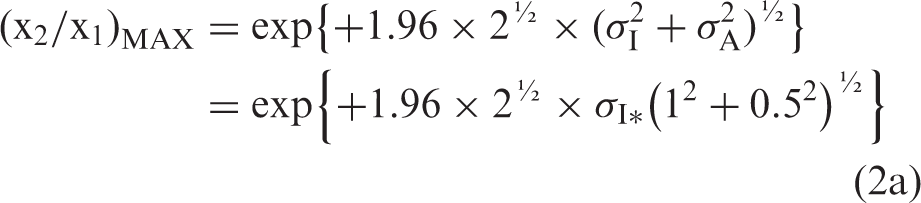
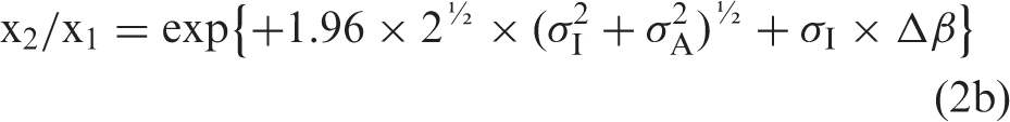
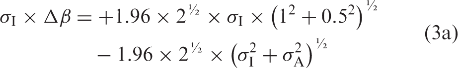
If the formulae using Gaussian distributions^4,5,7 are relevant also for ln-Gaussian distributions, then the relation between Δβ and σ_A is

${\sigma }_{\text{I}}\times \Delta \beta =+1.96\times 2\times {\sigma }_{\text{I}}\times (12+0.52)\mathrm{\hspace{1em}\hspace{1em}\hspace{1em}}-1.96\times 2\times ({\sigma }_{\text{I}}^2+{\sigma }_{\text{A}}^2)$

(3a)

${\sigma }_{\text{I}}\times \Delta \beta =+3.10\times {\sigma }_{\text{I}}-2.77\times ({\sigma }_{\text{I}}^2+{\sigma }_{\text{A}}^2)$

(3b)

${\sigma }_{\text{I}}\times \Delta \beta =+3.10\times {\sigma }_{\text{I}}-2.77\times ({\sigma }_{\text{I}}^2+(\text{x}\times {\sigma }_{\text{I}})2)$

(3c) where σ_A = x × σ_I and x varies between 0.0 and 0.5.

Back transformation from logarithms is performed by a BIAS_FACTOR

${\text{BIAS}}_{\text{FACTOR}}=\text{exp}\{{\sigma }_{\text{I}}\times \Delta \beta \}$

(4a) which gives the allowable limit for x₂/x₁, and further to the fractional bias BIAS_FRACTIONAL (not the concentration bias as related to standard deviations)

${\text{BIAS}}_{\text{FRACTIONAL}}={\text{BIAS}}_{\text{FACTOR}}-1$

(4b) which gives the allowable fractional (or percentage) deviation for (x₂ − x₁)/x_1.

Results

The test for our model will be that the ratio between the variable x₂/x_1, (x₂/x₁)_VAR and (x₂/x₁)_MAX is equal to 1.0, which is the same as

$({\text{x}}_2/{\text{x}}_1{)}_{\text{VAR}}/({\text{x}}_2/{\text{x}}_1{)}_{\text{MAX}}=\text{exp}\{+1.96\times 2\times ({\sigma }_{\text{I}}^2+{\sigma }_{\text{A}}^2)\mathrm{\hspace{1em}\hspace{1em}\hspace{1em}}+{\sigma }_{\text{I}}\times \Delta \beta \}/\text{exp}\{+1.96\times 2\mathrm{\hspace{1em}\hspace{1em}\hspace{1em}}\times {\sigma }_{\text{I}}\times (12+0.52)\}=1.0$

(5)

The bias factor, BIAS_FACTOR, then is BIAS_FACTOR = exp{#x003C3;_I × Δβ} and the fractional bias, BIAS_FRACTIONAL, becomes ${\text{BIAS}}_{\text{FRACTIONAL}}={\text{BIAS}}_{\text{FACTOR}}-1$ .

For the lower limit, the same formulae is based on z = −1.96

$({\text{x}}_2/{\text{x}}_1{)}_{\text{VAR}}/({\text{x}}_2/{\text{x}}_1{)}_{\text{MAX}}\mathrm{\hspace{1em}\hspace{1em}\hspace{1em}}=\text{exp}\{-(1.96\times 2\times ({\sigma }_{\text{I}}^2+{\sigma }_{\text{A}}^2)+{\sigma }_{\text{I}}\times \Delta \beta )\}\mathrm{\hspace{1em}\hspace{1em}\hspace{1em}\hspace{1em}\hspace{1em}\hspace{1em}}/\text{exp}\{-1.96\times 2{\sigma }_{\text{I}}\times (12+0.52)\}=1.0$

(6)

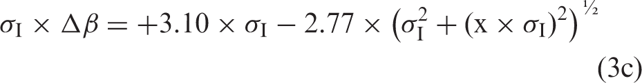
An example of logarithmic bias fraction, σ_I × Δβ =  +3.10 × σ_I−2.77 × (σ_I²+σ_A²)^½, as a function of σ_A = x × σ_I values from 0.00 to 0.15, for a σ_I-value = 0.3, is shown in Figure 1.

Figure 1.

An example of logarithmic bias fraction, σ_I × Δβ = + 3.10 × σ_I − 2.77×(σ_I²+ σ_A²)^½, as a function of σ_A = x × σ_I values from 0.00 to 0.15, for a σ_I-value = 0.3.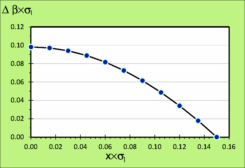

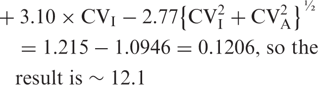
The Δβ is transformed to the BIAS_FACTOR = exp{#x003C3;_I × Δβ} = exp{#x0002B;1.96 × 2^½ × σ_I × (1²+ 0.5²)^½− 1.96 × 2^½ × (σ_I²+ σ_A²)^½} = exp{#x0002B;3.10 × σ_I − 2.77 ×  (σ_I²+ σ_A²)^½}. The relation between σ_I and maximum BIAS_FACTOR for maximum Δβ (i.e. σ_A = 0) is shown as a straight line in Figure 2. BIAS_FACTOR = exp{0.33 × σ_I} and the formula is maximum BIAS_FACTOR − 1, which is the same as the maximum fractional bias, BIAS_FRACTIONAL and the maximum fractional bias for σ_I = 0.1 is BIAS_FRACTIONAL = exp{0.33 × 0.1}−1 = 1.0335–1 = 0.0335 (≈ 3.35%).

Figure 2.

The relation between σ_I and the maximum bias factor. The relationship is described by the formula σ_I = exp{#x00394;β_MAX}.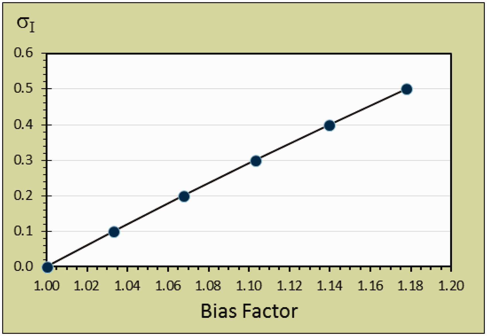

Example 1

Plasma prolactin with CV_I = 39.2% = 0.392. ¹¹

According to Lund et al., ⁹ CV_I is transformed to σ_I using the formula σ_I = {ln[CV_I²+ 1]}^½, σ_I = 0.378.

If a CV_A = 5.0% = 0.05 is assumed, the σ_A becomes 0.05, due to the small value where σ_I ∼ CV_I.

The allowable Δβ will become 0.378 × Δβ = +3.10 × σ_I − 2.77 × (σ_I²+ σ_A²)^½ = 1.1718–1.056 = 0.1156, and exp{0.1156} = 1.123, and BIAS_FRACTIONAL = 0.123, so the result is ∼ 12.3 %.

Figure 3 illustrates the relationships between the allowable bias fraction as function of σ_A between 0.00 and 0.05.

Figure 3.

Fractional bias as function of imprecision between 0.00 and 0.05 for plasma prolactin with CV_I = 39.2 % = 0.392 and transformed to σ_I using the formula σ_I = {ln[CV_I²+ 1]}^½, σ_I = 0.378.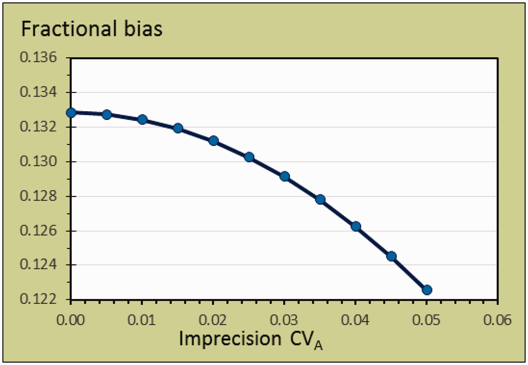

The traditional method^4,5 has no transformation of CV_I, since the assumption is for a Gaussian distribution, so the formula is

$+3.10\times {\text{CV}}_{\text{I}}-2.77\{{\text{CV}}_{\text{I}}^2+{\text{CV}}_{\text{A}}^2\}\mathrm{\hspace{1em}\hspace{1em}\hspace{1em}}=1.215-1.0946=0.1206,\text{sothe}\mathrm{\hspace{1em}\hspace{1em}\hspace{1em}}\text{resultis}~12.1\%$

or as standard deviations for a plasma prolactin concentration of 23 µg/L:

$+3.10\times 0.392\times 23\mu \text{g}/\text{L}-2.77\{0.3922+0.052\}\mathrm{\hspace{1em}\hspace{1em}\hspace{1em}}\times 23\mu \text{g}/\text{L}\mathrm{\hspace{1em}\hspace{1em}\hspace{1em}}=27.95\mu \text{g}/\text{L}-25.18\mu \text{g}/\text{L}=2.77\mu \text{g}/\text{L}$

which corresponds to a fraction of 2.77 μg/L/23 µg/L = 0.121∼12.1%.

Example 2

Plasma glucose with CV_I = 4.5 % = 0.045. ¹¹

According to Lund et al., ⁹ CV_I is transformed to σ_I using the formula σ_I = {ln[CV_I²+ 1]}^½ = 0.045 but, due to the small value, the result becomes indistinguishable from the CV_I.

If we assume a CV_A = 1.5% = 0.015, the σ_A becomes 0.015.

The allowable Δβ will become 0.045 × Δβ = 3.10 × 0.045 − 2.77 × (0.045²+ 0.015²)^½ = 0.1395–0.1314 = 0.0081, and exp{0.0081} = 1.0081, and BIAS_FRACTIONAL = 0.0081∼0.8 %.

The traditional method,^4,5 both as using s and CV, gives the same result: 0.8%.

Discussion

There are several indications that the distributions of both CV_I and CV_G are not Gaussian but skewed, as is the total variation of traditional population-based reference values for healthy individuals for many common measurands in laboratory medicine. Moreover, the use of logarithms is the basic assumption for the theoretical investigations both by Fokkema et al., ⁸ now widely cited and applied, and by Lund et al.^9,10 Even if the skewed distributions are better described by other possible models, we consider that logarithmic distributions are the best to describe numerical biological phenomena. In addition, the traditional description has drawbacks for large CV, e.g. the problems with negative concentrations being found when derived RCV are applied if inappropriately generated high CV are used. One of the reasons for the lack, to date, of clear and comprehensive documentation of the type of distribution may be the need for a large number of samples from healthy individuals in steady-state to reveal the exact type of distribution, whether Gaussian, ln-Gaussian or other.

Nonetheless, it is interesting to see that the performance specifications based on our new logarithmic and on the traditional ⁴ models are practical identical for small CV_I values such as for plasma glucose as documented in Example 2, and hardly dissimilar for plasma prolactin with large CV_I. This means that both models can be used for generating analytical performance specifications for CV – and corresponding s – except from the fact that only logarithmic models can avoid against negative concentrations being found when RCV are applied if large (but inappropriate) estimates of CV are used. The reason for the nearly identical results may be the transformation of CV_I to σ_I by the formula σ_I = {ln[CV_I²+ 1]}^½. This does seem to be very effective since the allowable Δbias for the plasma prolactin example (Example 1) would be 12.1 % instead of the 12.3 %, if not transformed logarithmically.

Both models for generation of analytical performance specifications can be useful for manufacturers of instruments and reagents including calibrators, where each lot has a specific Δbias from the previous lot. This is also vital for medical laboratories, where every change of lot poses a challenge to the desired analytical stability, and therefore needs special attention with necessity of intensive control, especially for measurands such as serum sodium, calcium and chloride which have well-documented small CV_I. In spite of the enormous endeavours on standardization of measurements with traceability to a high level of trueness, actual performance in practice may demonstrate large deviations, e.g. for serum sodium measured over eight years in two large Belgian hospital laboratories, where deviations of up to 4 mmol/L were seen. ¹² It is important to keep in mind that both Δβ and σ_A are variables in the formula and that their influences are fundamentally different: in consequence, solving problems and errors in ongoing analytical performance must be addressed separately for each variable.

Another model for RCV related to the change in standard deviation has been described by Jones ¹³ that RCV% = z × [CV_total²+ ((1 + RCV%) × CV_total)²]^½. This is complicated to calculate the limits for the RCV, but it might be interesting to estimate the performance specifications derived from this model and compare to our models in future work.

The estimation of analytical performance specifications with our new model seems to be rather more complicated than the traditional theory,^4,5 but, even for large CV_I, the difference between models is negligible; thus, only for very high CV_I is the ln-model of significant advantage.

Conclusions

Our model for analytical quality specifications based on logarithmic distributions of CV_A is conceptually more correct than the traditional model based on data derived using assumptions of Gaussian distributions, but results are similar up even with large CV_I.