Sage Journals: Discover world-class research

Abstract

Proteins are biomolecules with characteristic three-dimensional (3D) arrangements that render them different vital functions. In the last 20 years, there has been a growing interest in biopharmaceutical proteins, especially antibodies, due to their therapeutic application^. The functionality of a protein depends on the preservation of its native form, which under certain stressing conditions can undergo changes at different structural levels that cause them to lose their activity.¹ Although mass spectrometry is a powerful technique for primary structure determination, it often fails to give information at higher order levels. Like infrared (IR), Raman spectra are well known to contain bands (especially the amide I from 1625–1725cm^–1) that correlate with secondary structure (SS) content. However, unlike circular dichroism (CD), the most well-established technique for SS analysis, Raman spectroscopy allows a much wider ranges of optical density, making possible the analysis of highly concentrated samples with no prior dilution. Moreover, water is a weak scatterer below 3000 cm^–1, which confers Raman an advantage over IR for the analysis of complex aqueous pharmaceutical samples as the signal from water dominates the amide I region. The most traditional procedure to extract information on SS content is band-fitting. However, in most cases, we found the method to be ambiguous, limited by spectral noise and subjected to the judgment of the analyzer. Self-organizing maps (SOM) is a type of self-learning algorithm that organizes data in a two-dimensional (2D) space based on spectral similarity and class with no bias from the analyzer and very little effect from noise. In this work, a set of protein spectra with known SS content were collected in both solid and aqueous state with back-scatter Raman spectroscopy and used to train a SOM algorithm for SS prediction. The results were compared with those by partial least squares (PLS) regression, band-fitting, and X-ray data in the literature. The prediction errors observed by SOM were comparable to those by PLS and far from those obtained by band-fitting, proving Raman–SOM as viable alternative to the aforementioned methods.

Graphical abstract

This is a visual representation of the abstract.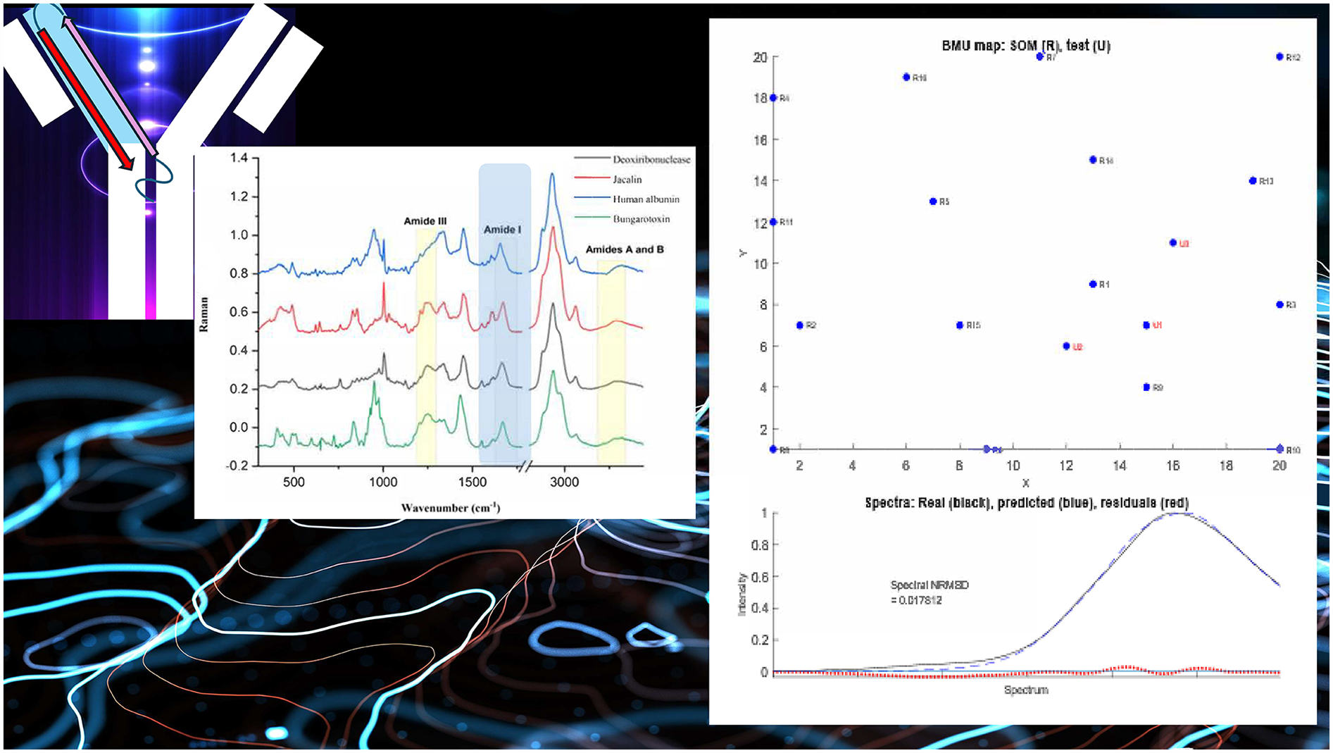

Keywords

Secondary structure of proteins Raman spectroscopy self-organizing maps SOM circular dichroism spectroscopy infrared spectroscopy‌

Introduction

Raman spectroscopy is a technique that measures the amount of energy exchanged when the electric field of an electromagnetic wave deforms the charge distribution in a molecule.^2,3 Raman spectroscopy usually involves shining visible light on a sample and measure the scattering that involves changes in vibrational energy levels. Thus the resulting spectra provides valuable information on the vibrations and hence structure of a molecule.⁴ Like infrared (IR) spectroscopy, Raman spectroscopy gives vibrational data for proteins that vary with the secondary structure (SS) content of globular proteins^.^5,6 The characteristic IR amide bands (A, B, I and III) are also active in Raman spectroscopy with the amide I (between 1625 and 1725 cm^–1) and III (between 1230 to 1300 cm^–1) being the most prominent ones and of biggest interest for SS prediction^5,6 (Figure 1). The correlations of these bands with SS was established in the 1970s based on studies of induced alpha-to-beta transitions of poly-L-lysine and comparative analysis with X-ray and CD spectroscopy of proteins.^7,8 Many methods exist in the literature to extract information on SS content from Raman spectra reviewed and collected by Bandekar^6,8–12 being band-fitting the most popular amongst them. However, the accuracy of SS predictions from protein Raman spectrum using band-fitting is not high due to both, the strong overlap between the SS assignments, and the risk of fitting noise when the SNR is low. We therefore considered alternative analysis methodologies used with success in infrared spectroscopy. The SS annotations used in this work are those assigned by the Define Secondary Structure of Proteins (DSSP) algorithm (https://2struc.cryst.bbk.ac.uk/twostruc), which divides secondary structure into eight major classes abbreviated as follows: 3₁₀-helix (G), α-helix (H), π-helix (I), β-sheet (E), β-bridge (B), turn (T), bend (S) and random coil (C).¹³ Out of the three different helical contents, alpha is the most common helical structure. We will refer to the total helical content as “helix” or “alpha” indistinctively throughout the document. All trainings were performed with five structures: helical, beta, turns, bends and random coil. However, because helical and beta contents are the major contributors to the structure, it was decided to focus the analysis on those two types of structures only.

Figure 1.

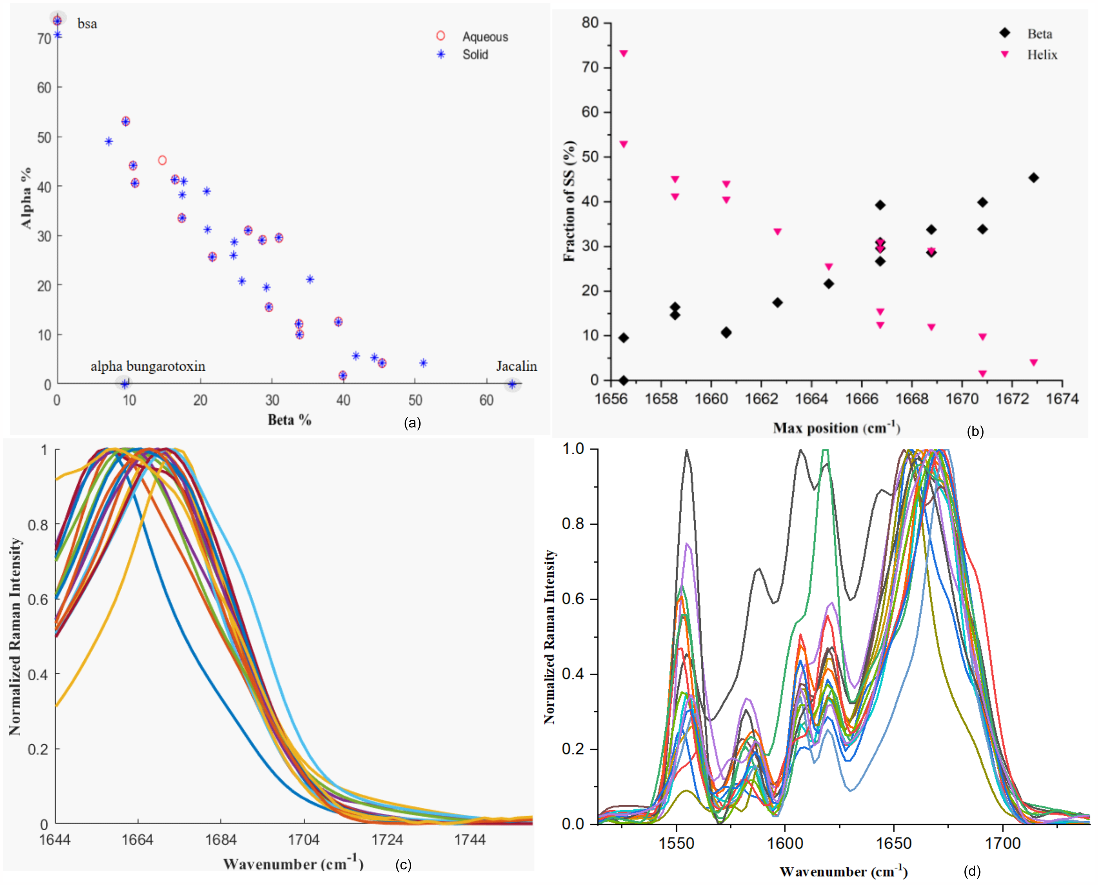
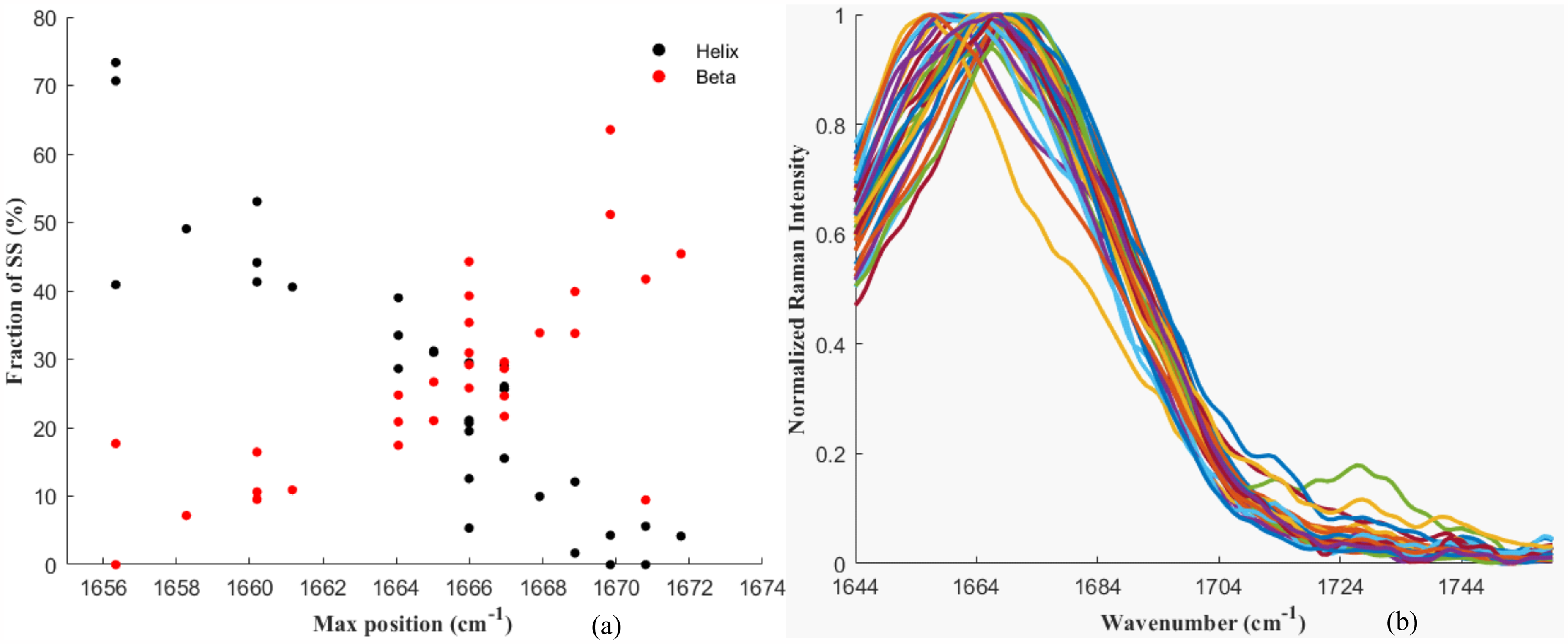
Alpha versus beta coverage of Raman reference set in aqueous and solid state based on 2struc annotations (a), alpha and beta contents in% versus amide I peak positions for spectra in the aqueous state (b), processed spectra in the range of the amide I corresponding to the proteins in aqueous state (c), and processed spectra in the range used for the band fitting analysis (d).

Raman can be measured in both highly concentrated aqueous samples and powders, which makes it a suitable alternative to CD spectroscopy.⁸ Moreover, the interference from the water vibrational mode in the region of the amide I is much smaller in Raman than in IR spectra, which makes predictions less influenced by errors resulting from water subtraction.^14,15 Although Raman spectroscopy offers many benefits compared to other spectroscopic techniques, impurities^16,17 can produce large amounts of fluorescence resulting in saturation of the Raman signal.¹⁴ There are a variety of techniques for suppression of background fluorescence but photobleaching, because of its simplicity, is the most popular approach and the one used in this work.^18–20 It is also generally believed that side chain contributions to spectra reduce the accuracy of SS prediction.

In this work, we focused our efforts in compiling a set of protein Raman spectra to train a self-organizing map (SOM) algorithm that was first implemented for CD spectroscopy and has already been used before for IR spectroscopy analysis.²¹ A SOM is a type of neural network architecture created by Kohonen²² that produces a 2D representation of a higher dimensional space and helps the visualization and hence identification of structures.^23,24 The new space or map is discrete and consists of nodes disposed in layers of arrays, each of them with unique spectral features and a SS assignment based on which the SS of a unknown can be determined by similarity.²⁴ SOM is a high dimensionality reduction technique that does not do projections in opposition to partial least squares regression (PLSR), which means the clusters they form are purely due to spectral features rather than correlations between properties associated with them. This means quantification of any other given property correlated with the amide I or any other spectral signature for that matter, would not require rebuilding the map. We evaluate the SOM performance in comparison with PLS, and band-fitting. PLS is a high-dimensionality reduction technique used for modelling.²⁵ PLS operates by building a new space consisting of orthogonal latent variables (LVs) where the spectra are projected. The SS can then be modelled based on the scores of the spectra in those latent variables.

Experimental

Materials and Methods

All of the proteins used were purchased from Sigma-Aldrich and any dilution and blank measurement was carried out with Milli-Q (ultra-pure) water. The number of proteins were 17 and 32 in aqueous and solid states, respectively (Table S1, Supplemental Material). The set of reference proteins was selected to ensure the coverage of the two main protein structures: alpha-helices and beta-strands. The aqueous-state set was limited by the solubility of the proteins in water. Also, the spectra of those proteins consisting of a heme group could not be obtained because of the interference of signals arising from the pyrroline ring (Figure S2, Supplemental Material).

Instrumentation

The instrumentation used consisted of a centrifuge Sigma D-37520 14k, Millex-GV 0.22 µm syringe filter disks, a syringe, Ika Vortex Genius 3, a marble mortar, a set of 40 × 40 × 40 mm³ quartz cuvettes from Starna, as well as Jasco 660 ultraviolet–visible (UV–Vis), FP 6500 fluorescence, and 1500 circular dichroism (CD) spectrometers.

The instrument used for the collection of Raman spectra of proteins in aqueous state was a BioTools Chiral Raman-2X Raman optical activity (ROA) spectrometer equipped with a 532 nm neodymium-doped yttrium aluminum garnet (Nd:YAG) laser of up to ∼1000 mW at sample position. This instrument measures Raman and ROA²⁶ simultaneously in the range 200–2300 cm^–¹. The instrument was aligned and calibrated prior to the measurements. The alignment involved the optics that define the path of the beam up to the sample, the position of the sample holder, the position of the fiber optics and the position of the camera; and was intended to maximize both the irradiance on the sample and the collection of the corresponding backscattered light. The y (intensity) and x (wavenumber) axes were manually calibrated using a fluorescent green glass and a Ne lamp, respectively.

The instrument used for the acquisition of the Raman spectra of proteins in solid state was a Thermo Fisher DXR Raman spectrometer equipped with a 633 nm He laser with an output of ∼8 mW at sample position and a 50 to 3500 cm^–1 detection range. Calibration and alignment were fully automated and performed weekly.

Experimental Procedure

For the aqueous-state protein reference set, the proteins were dissolved with water resulting in concentrations in the range 40–80 mg·ml^–1. The exact concentration was a consequence of both the amount of protein available and its solubility. All samples were centrifuged for 5 min at about 10 000 rpm to remove any undissolved protein. The eluent was recovered and filtered with a Millex-GV disk filter of 0.22 µm diameter to further remove any solid particles in suspension. About 40 µl of the stock solutions were used for the Raman measurements. A few samples did not require photobleaching, but the ones that did were exposed to the laser for periods that depended on the amount of fluorescence displayed. Although it is true that the rate at which fluorescence decays depends on the incident power, we soon learnt that increasing the power with no mechanism to refrigerate the sample often led to its calcination. Because of this, we decided to photobleach mildly fluorescing samples with ∼550 mW for about 3–5 hours, whereas other samples that fluoresced intensely were irradiated with powers between 165 and 275 mW for up to 24 hours. The spectra were accumulated until the region of interest (amide I band) was well defined and did not visibly change from scan to scan. The power used for the measurements ranged from 440 to 550 mW and the exposure time was between 0.36 and 1.02 s, always seeking to maximize the signal without saturating the detector. The proteins exposed the longest to the laser, including photobleaching, were measured before and after the Raman measurement by CD and fluorescence to ensure no unfolding took place due to exposure to the laser (Figures S3–S5, Supplemental Material).

For the solid-state protein set, the protein powder was first ground in a mortar and then decanted into a quartz cuvette. The samples were photobleached externally with a home-made device consisting of two diode lasers (635 and 532 nm and ∼150 mW outputs)²⁰ for periods ranging from a few minutes to a few hours prior to the spectra acquisition.

Data Processing

The solid-state protein spectra only required a baseline subtraction to correct for fluorescence. The procedure used consisted of selecting points across the spectrum that were believed to be only due to fluorescence and interpolating between them with cubic polynomials in the range 1508–3500 cm^–1 for subsequent subtraction³ (Figure S6, Supplemental Material). This operation was performed in Origin.²⁷

The aqueous-state protein spectra had a contribution from the water O–H bending in the range of interest. Although this is far less intense than that in IR (Figure S7, Supplemental Material) it was found necessary to subtract the water contribution for all the aqueous-state proteins prior to baseline correction as for the solids.

The Raman intensity depends exponentially on the Raman cross-section as well as concentration and pathlength and for small values it can be approximated by the linear term of a series expansion²⁸ so the total Raman signal of a protein in water can be expressed as the contribution of both the water and the protein (Eq. 1). Also, because the BioTools instrument used for the collection of the proteins in aqueous form does not average out but simply accumulates the signal, the Raman signal measured was proportional to both exposure and number of accumulations (total exposure).

I^{p w} \propto I_{o}^{p w} \cdot t^{p w} (σ^{p} \cdot C^{p} + σ^{w} \cdot C^{w})

(1)

where I^pw is the Raman signal of the protein in water (p denotes protein, w denotes water), σ is the Raman cross section, C is concentration, t stands for total exposure time, and I_o is the incident power. And for just the water only,

I^{w} \propto I_{o}^{w} \cdot t^{w} \cdot σ^{w} \cdot C^{w}

(2)

and so, the Raman signal of the protein under consideration is:

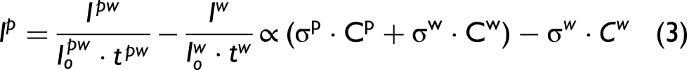
I^{p} = \frac{I^{p w}}{I_{o}^{p w} \cdot t^{p w}} - \frac{I^{w}}{I_{o}^{w} \cdot t^{w}} \propto (σ^{p} \cdot C^{p} + σ^{w} \cdot C^{w}) - σ^{w} \cdot C^{w}

(3)

As stated in Eq. 3, the spectra were divided by the laser power and the total exposure in order to scale them prior to water subtraction.

Like in solid state, the baselines of the different measured proteins were affected by fluorescence and thus a baseline correction was also required. The method employed for the aqueous spectra consisted of selecting anchor points that were attributed only to fluorescence that then were interpolated with cubic splines. A Matlab²⁹ routine was implemented to automate the scaling, subtraction.

Data Analysis

Partial Least Squares (PLS)

A PLS^30,31 algorithm was used to create a predictive model for the different structures by modelling the amide I band against their X-ray annotations (Tables S2–S3, Supplemental Material). The analysis was carried out in SOLO (Eigenvector Research Inc.)³² and leave one out cross-validation (LOOCV) was employed. The optimal spectral range, based on the predictive capability of the model, was found to be 1644.2–1759.4 and 1643.8–1700.7 cm⁻¹ for the aqueous and the solid form protein spectra, respectively. The same ranges were used for the SOM analysis.

Self-Organizing Maps (SOM)

The SOM algorithm works in three steps: (i) It organizes the spectra of a reference set of proteins with well-known SS (Tables S2–S3, Supplemental Material) clustering them in terms of spectral similarity, given by the distance between the nodes on the map. (ii) It assigns the secondary structure to the nodes by sum weighing the contributions of the neighboring proteins. (iii) It tests the sample spectrum against the map by identifying the best matching unit (BMU) in terms of the distance in the spectral space and then works out the SS by sum weighing the SS of the top three matching nodes in terms of the distance on the map.²⁴

Band-Fitting

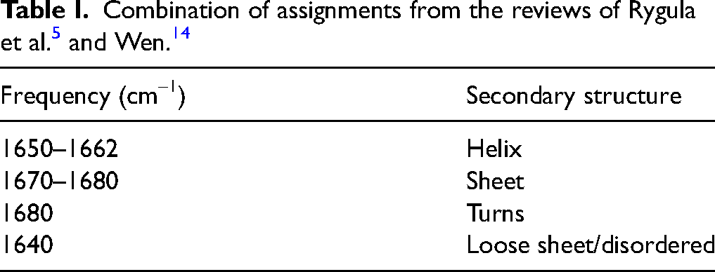
The amide I bands in aqueous state were bandfitted with combinations of Gaussians following similar protocols to those developed for the analysis of IR amide I bands.³³ In order to account for the influence of the aromatic side chains, which are strongly overlapped with the amide I, all the bands in the range from 1515 to 1740 cm^–1 were fitted together with the amide I and only the peaks within the range of the amide I used to compute the SS contents (Figures S26–S42, Supplemental Material).⁶ Prior to the analysis, the spectra were Fourier self-deconvolved to resolve as much as possible the intrinsic bands within the amide I peak. Constraints were set for the bandwidths, peak positions, and the intercepts (10−41 cm^–1, ± 3 cm^–1, and 0, respectively), but not for the number of bands, those were determined from the second derivative. The different bands within the amide I were assigned to different SS motifs in accordance with the literature and the overall contents determined by computing the ratios of the areas for each of the structures.³³ The assignments for the different structures can be found in Table I. The characteristic frequencies for helical and disordered content are the same as in IR spectroscopy. However, beta content can be found in the range 1670−1680 cm^–1, higher frequencies than that in IR spectroscopy (∼1620−1640 cm^–1).^21,33 The solid form protein spectra were not band-fitting due to the large levels of noise.

Table I.

Combination of assignments from the reviews of Rygula et al.⁵ and Wen.¹⁴

Frequency (cm^–1)	Secondary structure
1650–1662	Helix
1670–1680	Sheet
1680	Turns
1640	Loose sheet/disordered

Results and Discussion

Figure 1a shows the structure coverage of both the solid and aqueous data sets. The main two structures, alpha-helices and beta-strands, are strongly correlated. Although the coverage was good in general, there were some depleted areas, especially in the range 55–73% and 0–10% for alpha and beta contents, respectively, in both aqueous and solid state. Alpha bungarotoxin is the only protein that falls significantly off the linear trend due to both helical and beta structure contents (encircled). Jacalin and bovine serum albumin (BSA), with extreme beta and helical contents respectively, also seem to depart from the linear trend (also encircled).

Aqueous State

An exploratory analysis was conducted on Raman aqueous state spectra to determine the correlations between SS and the amide I band. The wavenumber corresponding to the maxima of the peaks were plotted against the helical and beta contents (Figure 1b). In agreement with the literature,^5,14 beta and helix structures were found to trend to 1672 and 1656 cm^–1, respectively.

The spectra of the aqueous-state protein set can be seen in Figures 1c–d. The proteins that were more exhaustively photobleached were scanned using CD before and after to ensure no degradation took place due to the increase in temperature (Figures S3–S5, Supplemental Material).

PLS Analysis

The best predictions, from the root mean square error (RMSE, Eq. 4) and determination coefficient for the goodness of fit (R², Eq. 5) values of the fittings were obtained in the range 1644.2–1759.4 cm^–1.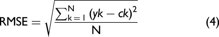

RMSE = \sqrt{\frac{\sum_{k = 1}^{N} {(y k - c k)}^{2}}{N}}

(4)

R^{2} = 1 - \sqrt{\frac{\sum_{k = 1}^{N} {(y k - Y k)}^{2}}{N - 1}}

(5)

where y_k is the predicted content, c_k the actual content, Y_k the value along the calibration curve, and N the total number of samples.

Additionally, to the processing discussed in the methods section, both the y (structures) and x (amide I spectra) matrix were mean centered prior to the analysis. The PLS was also attempted on the set scaled by area, which lead to slightly better predictions for alpha at the cost of those of beta (∼3%). Therefore, we decided to use the processing discussed in the methods section.

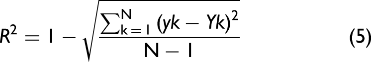
A LOOCV was performed with the first latent variable (Figure S7, Supplemental Material), which explained 81.6% of the variance in the matrix with the SS annotations and 68.76% of the spectral variance. The LOOCV predictions for each structure are represented against their X-ray annotations in Figure 2a. It was found that the predicted alpha and beta structures are strongly correlated with the X-ray annotations (indicated by the R² values, 0.824 and 0.839 for alpha and beta respectively) and that the mean errors (expressed as RMSE) are 7.9% for alpha and 5.04% for beta.

Figure 2.

Predicted alpha and beta structures by PLS versus X-ray annotations from (a) 2struc, (b) predicted alpha and beta structures by SOM versus X-ray annotations from 2struc, and (c) predicted alpha and beta structures by fitting versus X-ray annotations from 2struc.

SOM Analysis

Following the PLS analysis, the spectra and their X-ray annotations for SS content were used to train a SOM map. Figure 2b shows the correlation between the predictions and the annotations used to build the map. The error in the predictions for BSA was large compared to that of other proteins in the set and thus it was removed from the figure, which resulted in a significant improvement of both statistical metrics R² and RMSE. This poor predictions for BSA can be explained by the lack of representation of highly helical proteins in the reference set when BSA was removed from the set for the LOOCV and might be improved by including proteins in the set with similar SS content. The values for the determination coefficients came out to be 0.80 and 0.75, for alpha and beta structures, respectively. A bias in the intercept between alpha and beta structures could be observed in Figure 2b. That bias results from the inverse linear relationship between helical and beta structures (Figure 1a). The more the model overpredicts one type of structure, the more it will underpredict for its counterpart. The SOM maps and the fits for the LOOCV can be found in the Supplemental Material (Figures S9–S25). Bsa had the highest NRMSD value (9.2%), which agrees with the high prediction error observed for it.

Band-Fitting Analysis

Figure 1d shows the spectral range used for the band fitting (1515 to 1740cm^–1). The bands were fitted simultaneously in order to account as much as possible for the interference from the aromatic side chains. The peaks fitted to the amide I of the different protein samples (Figures S26–S42, Supplemental Material) were assigned to different SS (Table I) and their relative contents plotted against their X-ray assignments in Figure 2c. The correlation coefficients found between the predictions and the actual contents for alpha and beta structure were ∼0.40 and ∼0.39, respectively, far below those obtained using PLS and SOM.

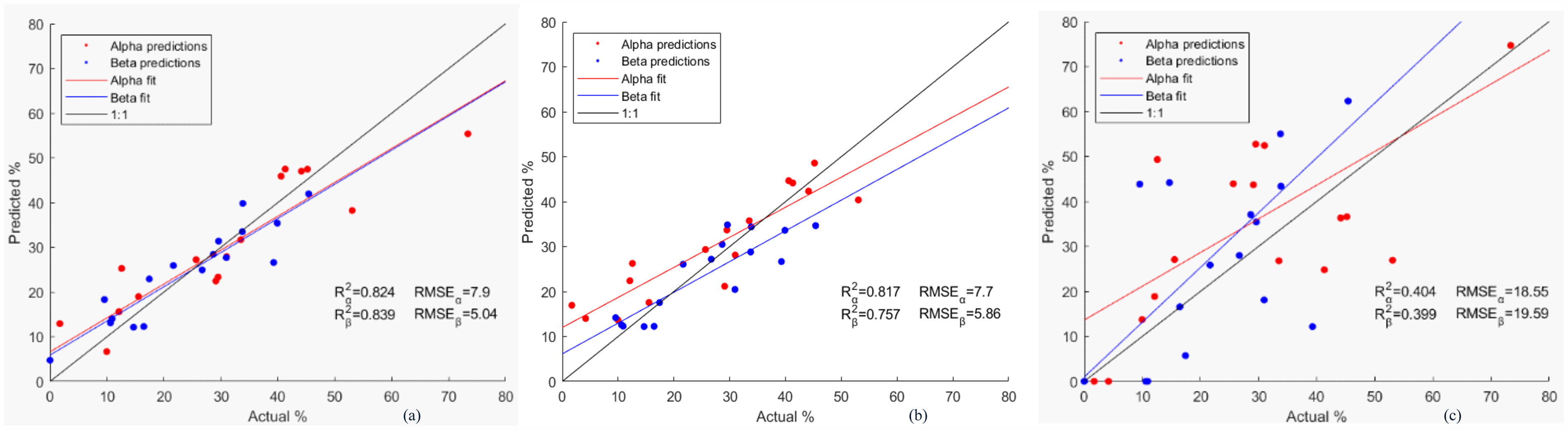
Figure 3 shows a comparison between the predictions for (a) alpha and (b) beta structures by the different methods and their X-ray annotations. In most cases, except for the helical contents of trypsin inhibitor and both helical and beta contents of beta lactoglobulin, when the PLS and SOM predictions are considerably close (less than 10% difference) their predictions seem to be representative of the X-ray annotation and hence, their average could be taken as the “true” SS content. In the event there is a large discrepancy between PLS and SOM (e.g., BSA) the estimates seem to benefit from the inclusion of band fitting as a tiebreaker, which averages closer to the X-ray value (presented in Figure 3 under the label “Average”). A compilation of the cumulative errors for the different methods can be found in Figure 3c, where it can be noticed the big disagreement between PLS and SOM with band fitting. Also, the average prediction errors for helical content came out positively skewed since both SOM and fitting resulted in slightly overpredicted helical structures too. The numerical values for every protein are given in the Supplemental Material section (Table I).

Figure 3.

Compilation of alpha (a) and beta (b) structure predictions for aqueous protein samples by SOM and PLS, band fitting, their average and X-ray annotations and, cumulative errors of predictions for aqueous samples by PLS, SOM, band fitting, and average (c).

Solid State

The spectra of the solid-state protein set can be seen in Figure 4b.

Figure 4.

SS annotations for helical and beta contents versus maxima of amide I band (a) and processed spectra corresponding to the protein in solid state (b). The range for the analysis was shortened down to 1643.8–1700.7 cm^–1.

The maxima of the amide I peaks of the solid form proteins were also plotted against the helical and beta contents (Figure 4a) confirming the trends found in aqueous form and literature: 1672 and 1656 cm^–1, for beta and helical contents, respectively. Another interesting fact that became more obvious from visual inspection of Figure 4a is that the trends seem to converge to the aforementioned values at about 50–55%, and that any additional increase in SS for either beta or helix will not result in further shift of the maxima of the amide I peaks, in agreement with what observed in liquid form (Figure 1b).

PLS Analysis

Partial least squares analysis was again performed, first to help determine the most ideal range for the analysis. It was found that the best correlation with the SS matrix was in the range from 1643.8 to 1700.7 cm^–1. The quality of the spectra degraded in comparison to that in aqueous form due to the limited laser output of the instrument used for both the photobleaching and the collection of the spectra. Predictions for protein 14 (alpha-bungarotoxin) were grossly off, so the protein was removed from the set and the analysis repeated. The reason for bungarotoxin gross errors could be attributed to the lack of capability of the model to make predictions out of the straight line showed in Figure 1a. Figure 5a shows how the predictions compare to the X-ray annotations in terms of predicted versus actual (R² = 0.856 and 0.743 and RMSE = 7.08 and 7.31 for alpha and beta, respectively).

Figure 5.

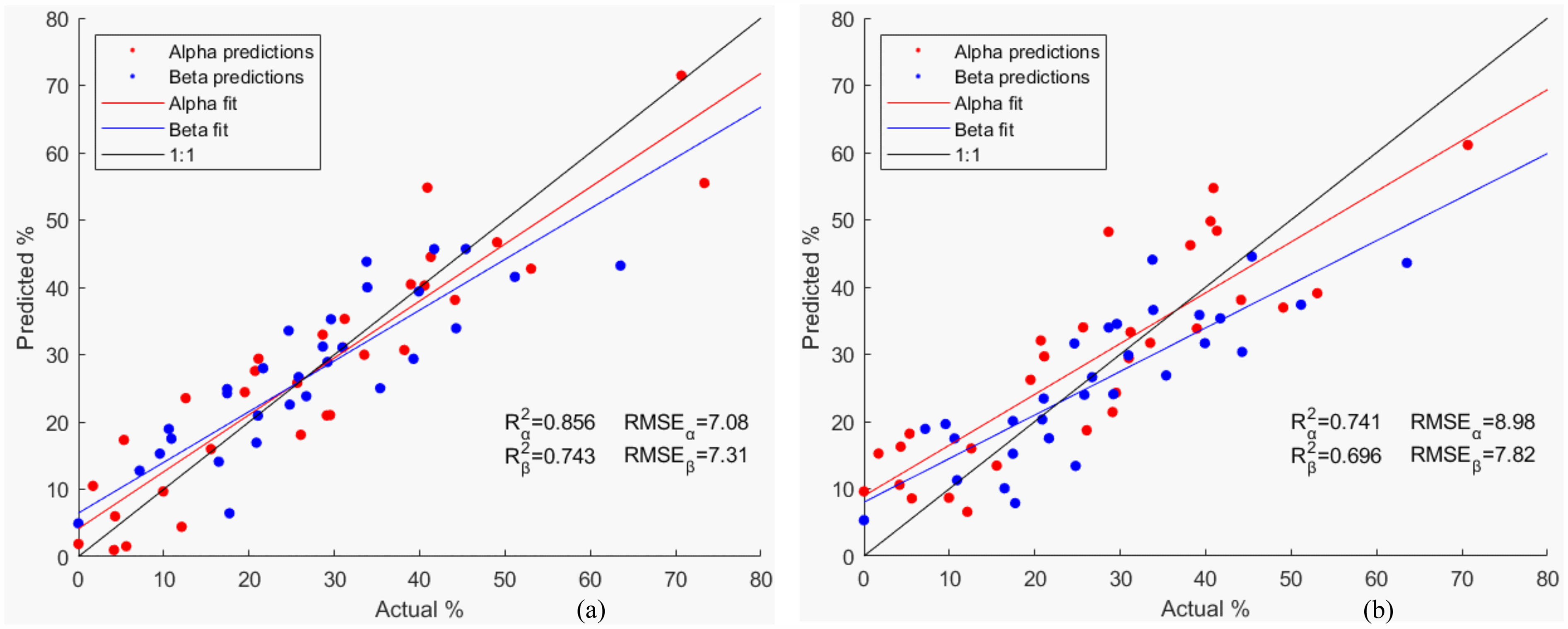
Predicted alpha and beta structures by PLS versus X-ray annotations from (a) 2struc for proteins in solid form and (b) predicted alpha and beta structures by SOM versus X-ray annotations from 2struc for proteins in solid form.

SOM Analysis

The data set was then used to train SOM maps using a LOOCV strategy. The predictions and their X-ray annotations are shown in Figure 5b. The presence of alpha-bungarotoxin was again detrimental for the model so it was removed from the set. As in aqueous form, the error in the predictions for BSA was large compared to that of other proteins in the set and thus, it was removed from the figure, which resulted in an improvement of the statistical metrics (R² = 0.741 and 0.696, RMSE=8.98 and 7.82, for alpha and beta respectively).

Figure 6 shows a comparison between the predictions for alpha (a) and beta (b) structures by the different methods and their X-ray annotations. In agreement with what observed before, the average of PLS and SOM predictions resulted in good (< 10% error) estimations of the X-ray annotations except for few of them, especially those with extreme SS contents (e.g., bovine fibrinogen, BSA for helix, and jacalin for beta). Those deviations could, again, be attributed to the lack of prediction capability out of the straight line in Figure 1a, and although both PLS and SOM predictions are affected by it, PLS seems to predict closer to the X-ray annotations for highly helical proteins such as human albumin and insulin, in opposition to highly beta content, where PLS did not seem to predict significantly better (e.g., alpha crystalline and jacalin). A compilation of the errors for the different methods can be found in Figure 6c, where it can be appreciated how the average improves the helical predictions, but does not make any noticeable difference in the beta predictions. The numerical values for every protein can be found in the Supplemental Material (Table S3).

Figure 6.

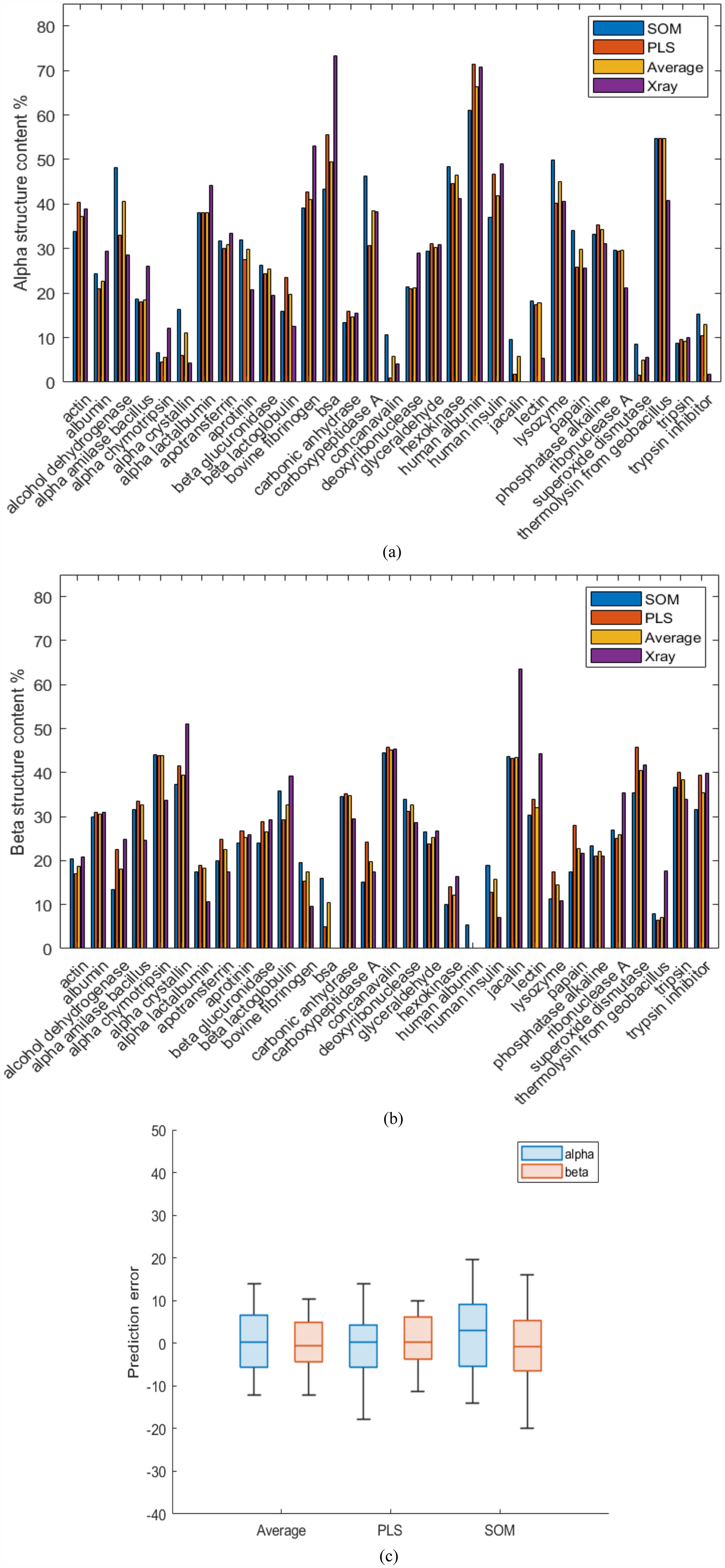
Compilation of (a) alpha and (b) beta structure predictions in solid form by SOM and PLS, their average and X-ray annotations, and (c) cumulative errors of predictions in solid form by PLS, SOM, and average.

Conclusion

It has been shown, in agreement with the literature, that there is a strong correlation between protein secondary structure content and the amide I Raman band. Different data analysis techniques were used to extract information on the SS content of a set of globular proteins in aqueous and solid form: PLS, SOM, and band fitting (only aqueous). The predictions by both PLS and SOM benefited from trimming the lower tail of the band (1625–1644 cm^–1), presumably due to the influence of the aromatic side chains.

In aqueous state, both PLS and SOM resulted in similar prediction errors, far smaller than those observed by band fitting. BSA was part of the calibration set when doing LOOCV by SOM, but its predictions turned out to be grossly inaccurate which we believe is due to lack of correlation between the amide I and the helical content above 50%. However, the predictions for BSA by PLS and band fitting came out to be ∼55% and ∼74% respectively, closer to the actual value of ∼73%, proving the benefit of using the three methods in a complementary manner.

In solid form, more proteins were available in the training set. The spectra were noisier compared to those in aqueous form, and the band-fitting approach could not be performed as a result. Also, due to the levels of noise, the spectra were subjected to a more exhaustive trimming in the upper part. Alpha-bungarotoxin threw gross errors and its presence proved detrimental for the predictive capabilities of both PLS and SOM models, so the decision was made to remove it from the training set, resulting in a significant improvement of the predictions. The better predictions were achieved by PLS, followed closely by SOM. BSA helical content by PLS came back again as ∼50%, and even lower by SOM. Jacalin beta content was also significantly underpredicted (∼ –20%).

To judge from these results, it could be said that both methods, PLS and SOM, are reliable alternatives to band fitting, and that their performance is the highest for helical and beta contents in the range ∼ 0–50%. Extremely high contents of SS cannot be accurately determined due to loss of correlation between amide I spectral features and SS content as it can be inferred from Figures 1b and 4a. Moreover, it seems like the PLS and SOM techniques would suffice for the purpose of SS determination of most globular proteins where the discrepancy between them is less than 10%, whereas in the event of bigger disagreements band fitting could be used as a tiebreaker. In all instances, the average of PLS and SOM or, PLS, SOM and band fitting is advised. Also, the use of the amide III in combination with the amide I could possibly help with the discrepancies found in this work between the different techniques and hence should be explored.

Supplemental Material

sj-docx-1-asp-10.1177_00037028251335051 - Supplemental material for Prediction of Secondary Structure Content of Proteins Using Raman Spectroscopy and Self-Organizing Maps

Supplemental material, sj-docx-1-asp-10.1177_00037028251335051 for Prediction of Secondary Structure Content of Proteins Using Raman Spectroscopy and Self-Organizing Maps by Marco Pinto Corujo, Pavel Michal, Dale Ang, Lindo Vivian, Nikola Chmel and Alison Rodger in Applied Spectroscopy

Footnotes

Acknowledgments

We would like to thank all those colleagues from the institutions the authors are affiliated with, in special to Josef Captain and Sophia C Goodchild.

Data Availability

The data that support the findings of this study are available on request from the corresponding author. The data are not publicly available due to privacy or ethical restrictions.

Declaration of Conflict of Interest

The author(s) declared no potential conflicts of interest with respect to the research, authorship, and/or publication of this article.

Funding

AR acknowledges funding from the Australian Research Council Industrial Transformation Training Centre in Facilitated Advancement of Australia’s Bioactives (Grant IC210100040). MP acknowledges funding from the Engineering and Physical Sciences Research Council via the Molecular Analytical Sciences Centre for Doctoral Training at the University of Warwick in UK (no. EP/L015307/1).

ORCID iDs

Marco Pinto Corujo

Dale Ang

Alison Rodger

Supplemental Material

All supplemental material mentioned in the text is available in the online version of the journal.

References

Hasija

Rahman

Ausar

S.F.

. “Forced Degradation Studies: an Essential Tool for the Formulation Development of Vaccines”. Vaccine: Development and Therapy. 2013. 3: 11–33. https://doi.org/10.2147/VDT.S41998

Ferraro

J.R.

Nakamoto

Brown

C.W.

. “Basic Theory”. In: Introductory Raman Spectroscopy. Amsterdam: Academic Press, 2003. Chap. 1, Pp. 14–26. https://doi.org/10.1016/B978-012254105-6/50004-4

Vandenabeele

. “Theoretical Aspects”. In: Practical Raman Spectroscopy: An Introduction. Chichester, UK: Wiley, 2013. Chap. 1, Pp. 1–7. https://doi.org/10.1002/9781119961284.ch1

Larkin

P.J.

. “Illustrated IR and Raman Spectra Demonstrating Important Functional Groups”. In: Infrared and Raman Spectroscopy. Amsterdam: Elsevier, 2011. Chap. 8, Pp. 135–176. https://doi.org/10.1016/B978-0-12-804162-8.00008-2

Rygula

Majzner

Marzec

K.M.

Kaczor

, et al. “Raman Spectroscopy of Proteins: A Review”. J. Raman Spectrosc. 2013. 44(8): 1061–1076. https://doi.org/10.1002/jrs.4335

Peters

Park

Kalyanaraman

Luczak

Ganesh

. “Protein Secondary Structure Determination Using Drop Coat Deposition Confocal Raman Spectroscopy”. Spectroscopy. 2016. 31(10): 31–39.

T.-J.

Lippert

J.L.

Peticolas

W.L.

. “Laser Raman Studies of Conformational Variations of Poly-L-Lysine”. Biopolymers. 1973. 12(9): 2161–2176. https://doi.org/10.1002/bip.1973.360120919

Lippert

J.L.

Tyminski

Desmeules

P.J.

. “Determination of the Secondary Structure of Proteins by Laser Raman Spectroscopy”. J. Am. Chem. Soc. 1975. 98(22): 7075–7080. https://doi.org/10.1021/ja00438a057

Williams

R.W.

. “Estimation of Protein Secondary Structure from the Laser Raman Amide I Spectrum”. J. Mol. Biol. 1983. 166(4): 581–603. https://doi.org/10.1016/S0022-2836(83)80285-X

10.

Bussian

B.M.

Sander

. “How to Determine Protein Secondary Structure in Solution by Raman Spectroscopy: Practical Guide and Test Case DNase I”. Biochemistry. 1989. 28(10): 4271–4277. https://doi.org/10.1021/bi00436a023

11.

Bandekar

. “Amide Modes and Protein Conformation”. Biochim. Biophys. Acta. 1992. 1120(2): 123–143. https://doi.org/10.1016/0167-4838(92)90261-b

12.

Maiti

N.C.

Apetri

M.M.

Zagorski

M.G.

Carey

P.R.

Anderson

V.E.

. “Raman Spectroscopic Characterization of Secondary Structure in Natively Unfolded Proteins: Alpha-Synuclein”. J. Am. Chem. Soc. 2004. 126(8): 2399–2408. https://doi.org/10.1021/ja0356176

13.

Kabsch

Sander

. “Dictionary of Protein Secondary Structure: Pattern Recognition of Hydrogen-Bonded and Geometrical Features”. Biopolymers. 1983. 22(12): 2577–2637. https://doi.org/10.1002/bip.360221211

14.

Wen

Z.Q.

. “Raman Spectroscopy of Protein Pharmaceuticals”. Pharm. Sci. 2007. 96(11): 2861–2878. https://doi.org/10.1002/jps.20895

15.

Kitagawa

Hirota

. “Raman Spectroscopy of Proteins”. In: P.R. Griffiths, J.M. Chalmers, editors. Handbook of Vibrational Spectroscopy. New York: Wiley, 2002. Pp. 3426–3446.

16.

Tan

S.C.

Yiap

B.C.

. “DNA, RNA, and Protein Extraction: The Past and the Present”. J. Biomed. Biotechnol. 2009. 2009: 574398. 10.1155/2009/574398

17.

Briggs

Panfili

P.R.

. “Quantitation of DNA and Protein Impurities in Biopharmaceuticals”. Anal. Chem. 1991. 63(9): 850–859. https://doi.org/10.1021/ac00009a003

18.

Macdonald

A.M.

Wyeth

. “On the Use of Photobleaching to Reduce Fluorescence Background in Raman Spectroscopy to Improve the Reliability of Pigment Identification on Painted Textiles”. J. Raman Spectrosc. 2006. 37(8): 830–835. https://doi.org/10.1002/jrs.1510

19.

Diaspro

Chirico

Usai

Ramoino

. “Photobleaching”. In: J.B. Pawley, editor. Handbook of Biological Confocal Microscopy. New York: Springer, 2006. Chap. 39, Pp. 690–702. https://doi.org/10.1007/978-0-387-45524-2_39

20.

Pinto Corujo

Michal

Wesson

Amarasinghe

D.P.

, et al. “Reduction of Background Fluorescence from Impurities in Protein Samples for Raman Spectroscopy”. J. Spectrosc. 2022. https://doi.org/10.1155/2022/1928091

21.

Pinto Corujo

Olamoyesan

Tukova

, et al. “SOMspec as a General Purpose Validated Self-Organising Map Tool for Rapid Protein Secondary Structure Prediction from Infrared Absorbance Data”. Front. Chem. 2022. 9: 784625. 10.3389/fchem.2021.784625

22.

Kohonen

. “The Self-Organizing Map”. Proc. IEEE. 78(9): 1464–1480. https://doi.org/10.1109/5.58325

23.

Zhu

. “Self-Organizing Map for Clustering Algorithms in Programming Codes”. In: 2010 Third International Conference on Business Intelligence and Financial Engineering. Hong Kong, China; 13–15 August 1990. Pp. 24–27. https://doi.org/10.1109/BIFE.2010.16

24.

Lasri

. “Clustering and Classification Using a Self-Organizing MAP: The Main Flaw and the Improvement Perspectives”. In: Proceedings of the 2016 SAI Computing Conference. London, UK; 13–15 July 2016. Pp. 1315–1318. https://doi.org/10.1109/SAI.2016.7556150

25.

Adams

M.J.

. “Calibration and Regression Analysis”. In: N.W. Barnett, editor. Chemometrics in Analytical Spectroscopy. Cambridge, UK: Royal Society of Chemistry, 2004. Chap. 6, Pp. 161–210. https://doi.org/10.1039/9781847550484-00161

26.

Barron

L.D.

. “A Historical Review of Optical Activity Phenomena”. In: Molecular Light Scattering and Optical Activity. Cambridge, UK: Cambridge University Press, 2004. Chap. 1, Pp. 1–52. https://doi.org/10.1017/CBO9780511535468.003

27.

OriginLab Corporation. “OriginPro 2025”. https://www.originlab.com/ [accessed 28 March 2025].

28.

Irish

D.D.

Adams

E.M.

. “Apparatus and Methods”. Am. Indust. Hyg Assoc. Quart. 1940. 1(1): 1–5. https://doi.org/10.1080/00968204009343768

29.

The Mathworks Inc. “Matlab”. https://www.mathworks.com/products/matlab.html https://eigenvector.com/software/solo/

30.

Steinbach

Anderson

C.A.

McGeorge

Inge

, et al. “Calibration Transfer of a Quantitative Transmission Raman PLS Model: Direct Transfer Versus. Global Modeling”. J. Pharm. Innov. 2017. 12(4): 347–356. https://doi.org/10.1007/s12247-017-9299-4

31.

Buckley

Matousek

. “Recent Advances in the Application of Transmission Raman Spectroscopy to Pharmaceutical Analysis”. J. Pharm. Biomed. Anal. 2011. 55(4): 645–652. https://doi.org/10.1016/j.jpba.2010.10.029

32.

Eigenvector Research Inc. “Solo”. https://eigenvector.com/software/solo/ https://eigenvector.com/software/solo/

33.

Yang

Kong

Dong

. “Obtaining Information About Protein Secondary Structures in Aqueous Solution Using Fourier Transform IR Spectroscopy”. Nat. Protoc. 2015. 10(3): 382–396. https://doi.org/10.1038/nprot.2015.024

Supplementary Material

Please find the following supplemental material available below.

For Open Access articles published under a Creative Commons License, all supplemental material carries the same license as the article it is associated with.

For non-Open Access articles published, all supplemental material carries a non-exclusive license, and permission requests for re-use of supplemental material or any part of supplemental material shall be sent directly to the copyright owner as specified in the copyright notice associated with the article.

0.00 MB

4.63 MB