Sage Journals: Discover world-class research

Abstract

Surface-enhanced Raman spectroscopy (SERS) has wide diagnostic applications due to narrow spectral features that allow multiplex analysis. We have previously developed a multiplexed, SERS-based nanosensor for micro-RNA (miRNA) detection called the inverse molecular sentinel (iMS). Machine learning (ML) algorithms have been increasingly adopted for spectral analysis due to their ability to discover underlying patterns and relationships within large and complex data sets. However, the high dimensionality of SERS data poses a challenge for traditional ML techniques, which can be prone to overfitting and poor generalization. Non-negative matrix factorization (NMF) reduces the dimensionality of SERS data while preserving information content. In this paper, we compared the performance of ML methods including convolutional neural network (CNN), support vector regression, and extreme gradient boosting combined with and without NMF for spectral unmixing of four-way multiplexed SERS spectra from iMS assays used for miRNA detection. CNN achieved high accuracy in spectral unmixing. Incorporating NMF before CNN drastically decreased memory and training demands without sacrificing model performance on SERS spectral unmixing. Additionally, models were interpreted using gradient class activation maps and partial dependency plots to understand predictions. These models were used to analyze clinical SERS data from single-plexed iMS in RNA extracted from 17 endoscopic tissue biopsies. CNN and CNN-NMF, trained on multiplexed data, performed most accurately with RMSE_label = 0.101 and 9.68 × 10^–2, respectively. We demonstrated that CNN-based ML shows great promise in spectral unmixing of multiplexed SERS spectra, and the effect of dimensionality reduction on performance and training speed.

Graphical abstract

This is a visual representation of the abstract.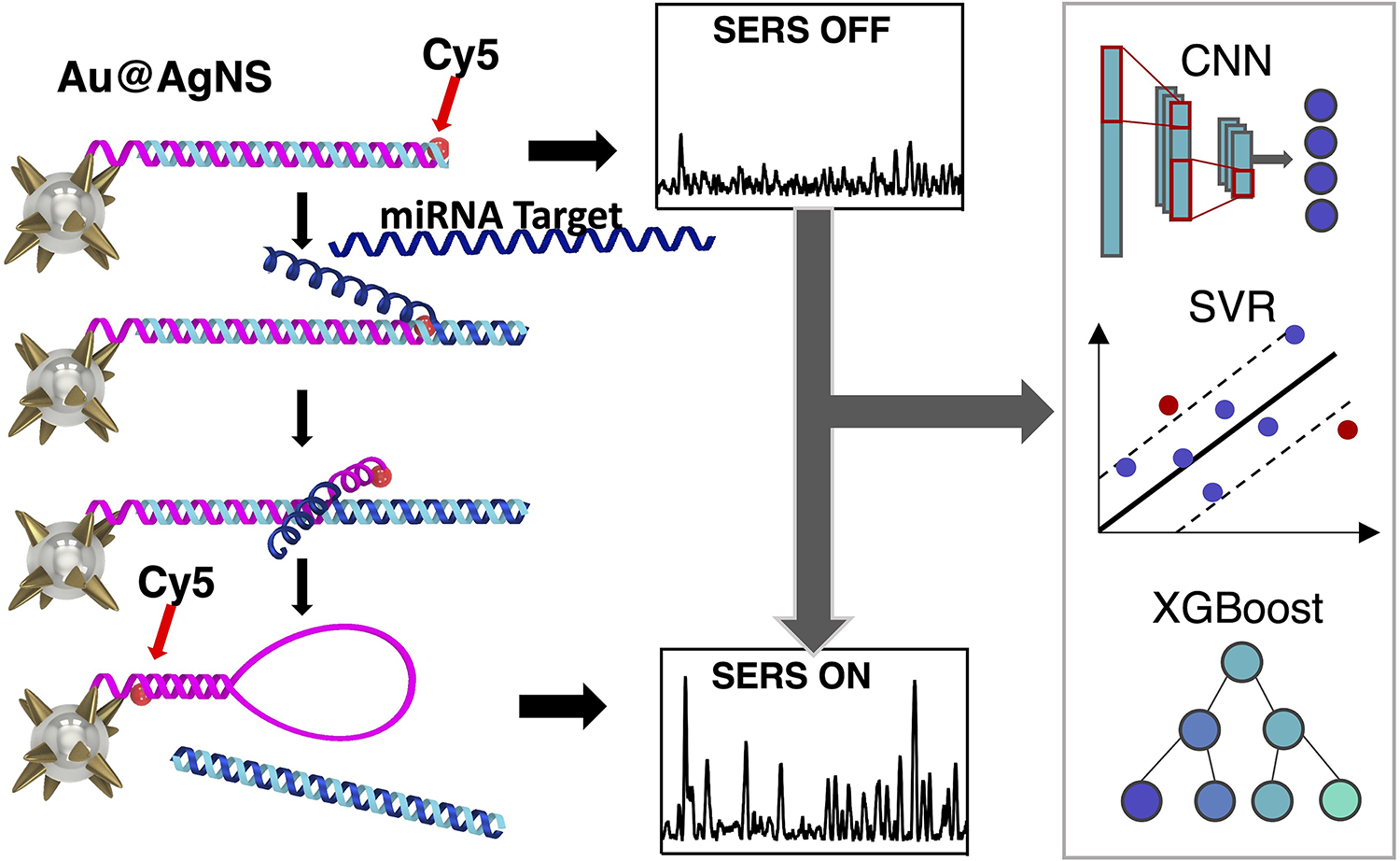

Keywords

Surface-enhanced Raman spectroscopy SERS micro-RNA miRNA machine learning non-negative matrix factorization NMF nanoparticle convolutional neural network CNN

Introduction

Surface-enhanced Raman spectroscopy (SERS) has been shown to be a powerful technique used for a variety of applications including imaging, chemical sensing, and biomedical diagnostics.^1–4 One of the key advantages of SERS is its so-called “fingerprint” spectra. SERS spectra have narrow, defined peaks based on the vibrational modes of the molecule, which make the technique particularly suited to multiplexed detection⁵ compared to more commonly used traditional techniques such as fluorescence. SERS is also highly advantageous due to its high sensitivity, allowing for single-molecule detection.⁶

Due to its distinct advantages, SERS represents a promising tool for molecular diagnostics. Over three decades, our laboratory has developed various SERS substrates and detection techniques ranging from chemical sensing^7–9 to molecular diagnostics.^10–14 The need for accessible strategies for early cancer diagnosis is critical, and nucleic acid-based molecular diagnostics, particularly micro-RNAs (miRNAs), show promise as biomarkers for early detection of various diseases including cancers,¹⁵ such as esophageal adenocarcinoma¹⁶ and colorectal cancer (CRC),¹⁷ cardiovascular disease,¹⁸ and neurogenerative diseases.¹⁹ These cancers have unique biomarker profiles, including miRNA-21, that can be detected in tissue and peripheral blood, but challenges with detection have prevented implementation in early diagnostics due to the need for specialized equipment and time-consuming processes. Despite recent developments in molecular diagnostics, there remains a gap between their advancement and their implementation in clinical settings. SERS-based diagnostic developments may help close the gap due to their high diagnostic accuracy and capability for multiplexed sensing.²⁰

We previously developed the “inverse molecular sentinel” (iMS) plasmonic nanobiosensor assay, which allows for highly sensitive and multiplexed detection of nucleic acids. IMS uses the sensing platform silver-coated gold nanostars (AuNS@Ag). Like gold nanostars, AuNS@Ag have the advantage of sharp tip geometry which produces a highly localized electric field enhancement, but AuNS@Ag produce even greater SERS enhancement over gold nanostars.²¹ The nanobiosensor detects a target nucleic acid sequence with an “off–on” signal produced by a non-enzymatic DNA strand-displacement process and stem-loop formation (Figure 1a). The nanobiosensor produces signal switching based on the spatial dependence of SERS intensity and involves two DNA probes: stem-loop probe and placeholder strand. Stem-loop DNA probes with a Raman label at one end are fixed to AuNS@Ag surface by a metal–thiol bond. As the name suggests, this stem-loop probe is designed to form two distinct geometries, switching the SERS signal on or off by bringing the Raman reporter physically closer or farther from the metallic surface. In the SERS OFF configuration, the stem-loop probe is hybridized to the placeholder strand with an overhang called the “toehold”. The target miRNA binds to the toehold region, initiating an energetically favorable strand displacement of the placeholder strand due to the higher melting temperature between the target and placeholder. This leaves the stem-loop probe to form a hairpin geometry, bringing the Raman dye close to the metallic surface and producing a strong SERS signal (SERS ON).

Figure 1.

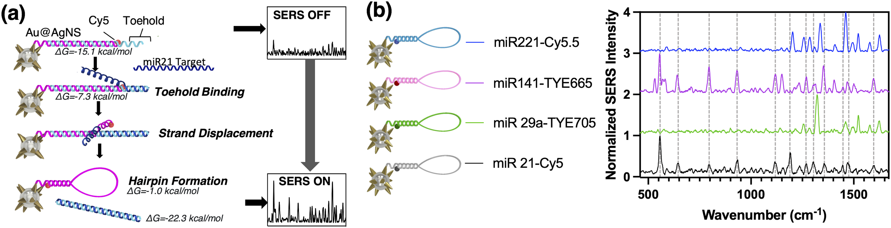
(a) Detection scheme of multiplexed SERS iMS nanoprobe. (b) Averaged reference spectra of each iMS sensor utilizing different Raman-active dyes: miRNA-221-Cy5.5 (blue), miRNA-141-TYE665 (pink), miRNA-29a-TYE705 (green), and miRNA-21-Cy5 (black). Vertical dashed lines show location of SERS peaks in miRNA-21-Cy5 iMS spectrum.

Micro-RNA-21 (miRNA-21) has been found to be a highly significant biomarker for esophageal cancers.²² iMS has demonstrated direct detection of the early cancer biomarker miRNA-21 from clinical samples without the need for target amplification.^13,14 Previously, we found that miRNA-21 in iMS alone achieved high diagnostic sensitivity, with 90% true positive and 100% true negative rates, and the area under the curve (AUC) of the receiver operating characteristic was 0.957.¹³ However, detecting a combination of these dysregulated miRNA targets increased their diagnostic and prognostic power. SERS is uniquely suited to this challenge due to its sharp peaks, which allow for high degrees of multiplexed detection. We developed iMS nanoprobe panels for the detection of four miRNAs that have been shown to be promising diagnostic biomarkers for CRC: miRNA-21, miRNA-29a, miRNA-221, and miRNA-141.^23,24 The multiplexed iMS detection of miRNA panels have transformative potential for applications in cancer research and future clinical applications for direct detection of miRNA in patient biopsies and biofluids.

Surface-enhanced Raman spectroscopy (SERS) is continually impacted by the ongoing machine learning (ML) revolution.²⁵ Dimensionality reduction techniques such as principal component analysis (PCA) and partial least squares are standard in spectral analysis.²⁶ However, as the degree of multiplexing continues to increase, accurate spectral unmixing becomes more crucial to accurate data interpretation. Additionally, at higher degrees of multiplexing, ML methods provide a greater accuracy improvement compared to standard methods.²⁷ ML methods including support vector machines (SVMs),^28,29 extreme gradient boosting (XGBoost),^30–32 and neural networks^27,33 are increasingly used for spectral analysis with improved accuracy. In recent studies, deep learning (multilayered) using convolutional neural networks (CNNs) is also more commonly applied for Raman and SERS data analysis.^27,34,35 In a previous study, we found that CNN analysis can provide superior accuracy compared to other ML and non-ML methods, followed closely by support vector regression (SVR);²⁷ however, CNN requires extensive computational power/training time. To reduce the number of features and thus computational power/training time needed, dimensionality reduction has been combined with CNN⁶ and other ML models. Another disadvantage of CNN is that it is often described as a “black box” due to its low interpretability. XGBoost is a boosted decision tree algorithm that is widely used as it is efficient, performs with high accuracy, and can be more easily interpreted through partial dependency plots (PDPs). Gao et al.³¹ found that XGBoost performed better than LightGBM and CatBoostLight in predicting lignan content. In this study, we investigate the accuracy of promising ML models applied to multiplexed iMS SERS spectra, the effect of dimensionality reduction on prediction accuracy, and model interpretability. We compared the performance of six ML models: CNN, SVR, and XGBoost with and without dimensionality reduction using non-negative matrix factorization (NMF). Then the performances of these ML models were compared to a standard method: spectral decomposition (SD).³⁶ We employed these models to decompose SERS spectra from a four-way multiplexed iMS assay using synthetic DNA targets. Then, we applied these models to an iMS assay used to detect miRNA-21 in patient samples. The results demonstrate the comparative performance of different ML methods and illustrate how combining ML with dimensionality reduction can lead to improved model performance and better predictions in SERS spectral unmixing.

Experimental

Materials and Methods

Gold(III) chloride trihydrate (HAuCl₄·3H₂O), l(+)-ascorbic acid, trisodium citrate dihydrate, sodium borohydride, 1 N hydrochloric acid (HCl) solution, phosphate-buffered saline (PBS), Tween-20, and 6-mercapto-1-hexanol (MCH) were purchased from Sigma-Aldrich at the highest purity grade available. Silver nitrate (AgNO₃, 99.995%) was supplied by Alfa Aesar. Thiol PEG (mPEG-SH, MW 5000) was purchased from Nanocs. Ammonium hydroxide (NH₄OH, 29.5%) was obtained from VWR. All oligonucleotides were purchased from Integrated DNA Technologies, Inc. All glassware and stir bars were thoroughly cleaned with aqua regia and dried prior to use. Ultrapure water (18 MΩ·cm) was used in all preparations.

Silver-Coated Gold Nanostar Synthesis

Silver-coated gold nanostars (AuNS@Ag) with s30Ag5 were synthesized using a previously described procedure.¹³ Briefly, a 12 nm gold-seed-solution was first prepared using a modified Turkevich method. AuNS were then synthesized by the simultaneous addition of 50 μL of 6 mM AgNO₃ and 50 μL of 0.1 M ascorbic acid to a solution containing 10 mL of 0.25 mM HAuCl₄, 10 μL of 1 N HCl, and 100 μL of the 12 nm gold-seed solution under gentle stirring at room temperature. The process was completed in less than a minute along with a color change from light orange to dark blue within 10 s, indicating the formation of AuNS. The stock concentration of AuNS is approximately 0.1 nM, as determined by nanoparticle tracking analysis (NTA 2.1, build 0342). The AuNS@Ag were prepared from the aforementioned procedure.¹³ For synthesis of AuNS@Ag, unfunctionalized AuNS were kept stirring and 50 μL of 0.1 M AgNO₃ and 10 μL of NH₄OH were added to the solution. The color of the solution changed from blue to dark brown. The obtained solution was used for further functionalization without purification. AuNS@Ag were functionalized 3 h after the synthesis to obtain iMS nanoprobes for nucleotide detection and imaging.

Probe Design

Inverse molecular sentinel (iMS) probes were designed using DINAMelt to simulate nucleic acid hybridizations and calculate melting temperatures. Four distinct sets or “flavors” of probes were designed for the detection of miRNA-21, miRNA-29a, miRNA-141, and miRNA-221. The sequences for the stem-loop and the placeholder were chosen to maximize the sensitivity by optimizing the melting temperatures of the probe–placeholder and placeholder–target hybrid complexes. The stem-loop and placeholder sequences were designed as shown in Table I. The stem-loop sequences for targets miRNA-21, miRNA-141, and miRNA-221 contain a 5′-thiol modifier and 3′ Raman dye. Due to the availability of dye conjugations for TYE705, the stem-loop contained a 5′ Raman dye and 3′-thiol modifier. The thiol termination allows for binding of the 5′ or 3′ end of the nanoparticle surface, respectively. The synthetic DNA targets are also shown in Table I.

Table I.

The molecular sentinel and placeholder DNA probe sequence designs for each multiplexed iMS “flavor” as well as the corresponding miRNA target: (a) miRNA-21, (b) miRNA-141, (c) miRNA-221, and (d) miRNA-29a. Bolded parts of the stem loop show hairpin binding regions, and bolded segment of the placeholder shows the toehold.

Target	Stem loop	Placeholder	Target
miRNA-21	5′-SH-AAAAAGTCTGTATTAAAAAATAGCTTATCAGAC-Cy5-3′	5′-TCAACATCAGTCTGATAAGCTATTTT-3′	5′-TAGCTTATCAGACTGATGTTGA-3′
miRNA-29a	5′-TYE705-TCTGAAATCGGTTAAAAAAAAAAAAATTCAGAAAAAA-SH-3′	5′-TTTTTAACCGATTTCAGATGGTGCTA- 3′	5′- TAGCACCATCTGAAATCGGTTA-3′
miRNA-141	5′-SH-AAAAACCAGAAAAAAAAAAAAAATAACACTGTCTGG-TYE665-3′	5′- CCATCTTTACCAGACAGTGTTATTTT- 3’	5′- TAACACTGTCTGGTAAAGATGG-3′
miRNA-221	5′-SH-AAAAAGCAGAATTAAAAAAAAAAGCTACATTGTCTGC-Cy5.5-3′	5’- GAAACCCCAGCAGACAATG TAGCTTTTT-3′	5′- AGCTACATTGTCT GCTGGGTTTC-3′

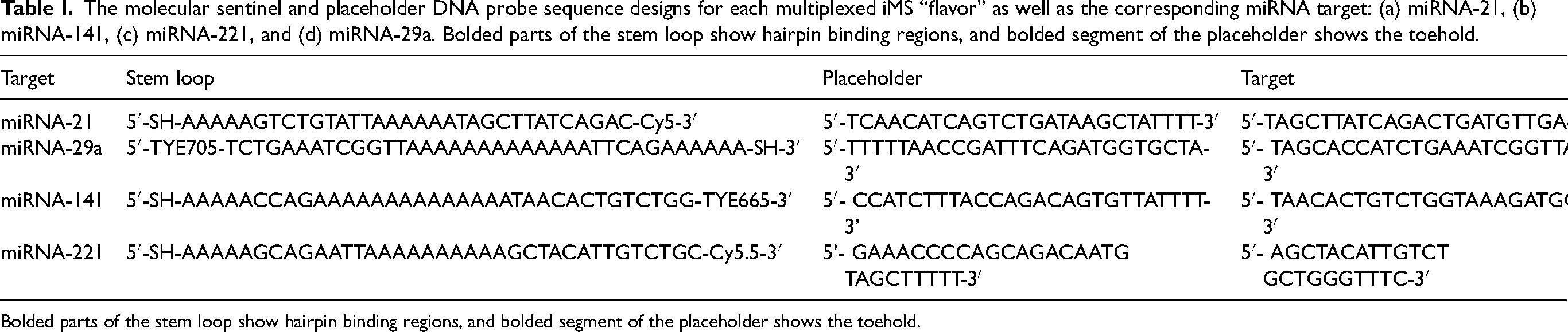
Bolded parts of the stem loop show hairpin binding regions, and bolded segment of the placeholder shows the toehold.

Inverse Molecular Sentinel Nanoprobe Synthesis

The iMS nanoprobes were synthesized following our previous publications, with minor adjustments using a pH-assisted method.^37,38 To adjust the pH of the prepared AuNS@Ag solution, a citrate buffer was prepared, consisting of 0.1 M sodium citrate dihydrate and 0.3 N HCl. The stem-loop probes were incubated with an excess of Tris(2-carboxyethyl)phosphine hydrochloride (TCEP) at room temperature for 1.5 h to reduce disulfide bonds. The TCEP-treated probe was then added to the prepared AuNS@Ag (one time) at a final concentration of 0.2 µM. The resulting mixture (0.9 mL) was sonicated briefly, followed by the addition of a citrate–HCl buffer (100 µL). After allowing the mixture to react at room temperature for 10 min, 10 µM Thiol-PEG (mPEG-SH, MW 5000) was added. The solution was left at room temperature for 30 min, then mixed with 1% Tween-20 (10 µL), subjected to centrifugation (9000 r/min, 10 min), and resuspended in a Tris-HCl buffer (10 mM, pH 8.0) containing 0.01% Tween-20. The nanostar surface was passivated with 0.1 mM MCH at 37 °C for 10 min, followed by four additional centrifugal washing steps using Tris-HCl buffer (10 mM, pH 8.0) containing 0.01% Tween-20. After the fourth centrifugation, the pellet was resuspended in 10 mM sodium phosphate buffer (pH 8.0) containing 0.01% Tween-20 (200 µL). For the preparation of iMS-OFF nanoprobes, the iMS-AuNS@Ag solution was incubated with 2 µM placeholder DNA in one time PBS buffer containing 0.01% Tween-20 at 37 °C for approximately 20 h. Excess placeholder strands were removed through four centrifugal washing steps (9000 r/min, 10 min), and the final resuspension was done in 1x PBS buffer containing 0.01% Tween-20. The iMS solution was then stored at 4 °C until further use.

Inverse Molecular Sentinel (iMS) Nanoprobe Characterization

To confirm AuNS@Ag morphology, nanoprobes were imaged using a transmission electron microscope (FEI Tecnai G2 twin TEM). ImageJ was used to analyze the size of n = 156 particles from a transmission electron micrograph (Figure S1, Supplemental Material). The AuNS@Ag had an average diameter of 72 ± 7 nm. To characterize nanoprobe optical properties, absorption spectra were acquired with a FLUOstar Omega plate reader (BMG Labtech GmbH) before and after functionalization (Figure S1, Supplemental Material). Functionalization with Cy5-stem loop and placeholder resulted in a 6 nm redshift of the absorbance peak from 518 to 524 nm due to the presence of Cy5 on the stem loop.

Inverse Molecular Sentinel (iMS) Assay Experimental Protocol

The iMS nanoprobe for detecting miRNA-21 was designed and synthesized with slight modifications from previous studies.^13,37 In the absence of the miRNA-21 target, the SERS signal of the iMS assay remains low, as the placeholder strands effectively maintain a linear duplex configuration, keeping the Raman label away from the AuNS@Ag plasmonic surface. When present, the miRNA-21 target provides a significantly increased SERS signal, indicating that the Raman labels are brought close to the nanoparticle surface and therefore experience the enhanced electromagnetic field. The iMS operating principle is schematically depicted in Figure 1a. In this study, we demonstrate four-way multiplexed detection using four unique iMS “flavors” (Figure 1b).

Spectral Acquisition of Multiplexed iMS Surface-Enhanced Raman Spectra for Calibration Curve and Test Set

Each multiplexed probe was combined at different final concentrations in the multiplexed-iMS solution: 5 pM miRNA-21-iMS and 25 pM miRNA-29a-iMS/miRNA-221-iMS/miRNA-141-iMS. Sensing concentrations were determined by the signal strengths of each individual iMS. In total, 80 μL of multiplexed iMS probes were combined with 20 μL synthetic DNA target obtained from the image dissector tube in a glass vial and incubated at room temperature with shaking for 1 h. The SERS measurement was obtained using a SERS spectrometer (Renishaw InVia) equipped with a 633 nm He–Ne laser, utilizing WiRE 2.0 software. Laser light travels through a laser line filter and focuses into the middle of the sample solution through the 10× microscope objective. A 633 nm laser excitation was used because dyes conjugated to stem loop were designed for excitation at 633 nm. Each sample was measured three times with one accumulation of 20 s for n = 48 test spectra. Test spectra were sorted into high signal-to-noise ratio (S/N) and low S/N subsets, or n = 28 and n = 20, respectively.

Reference Acquisition for Data Augmentation

Precisely, 80 μL of multiplexed iMS was loaded into a glass tube at the predetermined concentrations. Three blank SERS measurements were obtained using the above laser system. Then, 20 μL of a single synthetic DNA target was added to a multiplexed iMS solution, resulting in a final target concentration of 1 μM. After shaking incubation for 1 h, three SERS spectra were obtained for each distinct miRNA target. All SERS spectra were taken using the above laser system in the range 433–1776 cm^–1 with 10–30 s exposure time (Figure 2b).

Figure 2.

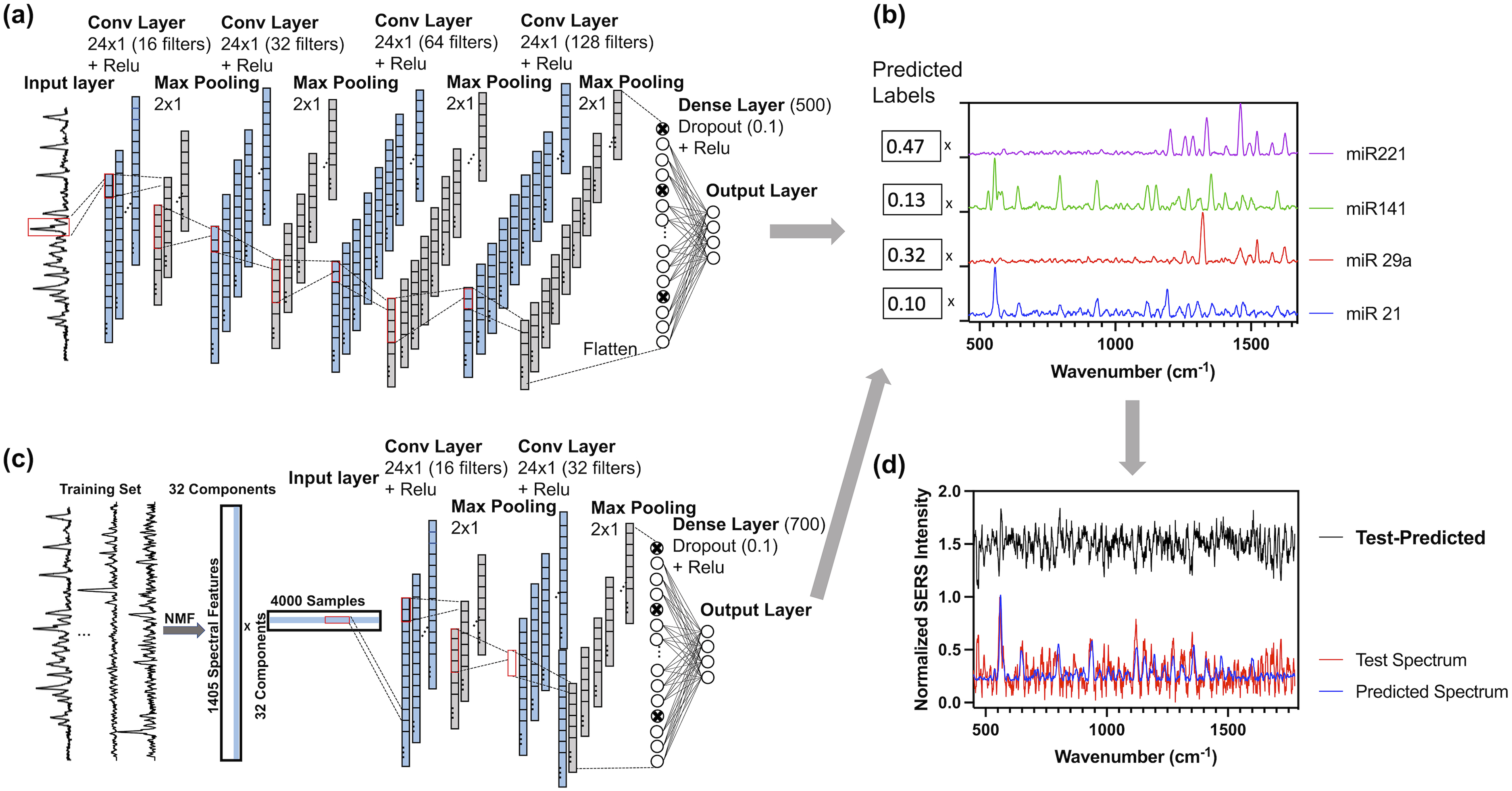
Schematic for CNN architecture (a) and NMF-CNN architecture (c). Output predicted labels are used for scaled addition of reference spectra (b) to reconstruct a predicted spectrum (d): normalized test spectrum is plotted in red, normalized predicted spectrum is plotted in red, and the difference between test and predicted spectra was plotted in black with an offset of 1.5.

Data Preprocessing

The entire sampled spectral range was used for training and testing. Each raw reference spectrum was blank subtracted, smoothed, and background-subtracted, using a Savitzky–Golay filter (five-point window and first-order polynomial) in Matlab.

Data Simulation

Training and validation data sets were simulated with modifications from a previous study.²⁷ Briefly, simulated spectral mixtures were made by mathematically combining reference spectra. Four reference spectra were acquired and used for each distinct iMS “flavor”. During data augmentation, one spectrum from each reference was randomly selected for use in mixture simulation. Data augmentation consisted of four steps: (i) separate the background from the raw spectrum; (ii) normalize raw spectrum by dividing by the max intensity of the background subtracted spectrum; (iii) scale normalized raw spectum by the simulated scaling factor (label); (iv) horizontally shift spectra a random number of spaces left or right in the range [0–4]; (v) add Gaussian noise at random power in the range (1 × 10^–5–1 × 10^–3); (vi) background subtraction in custom code with window 40; (vii) normalize background subtracted data so all spectral points are in the range [0–1]. An example of simulation steps is shown in Figure S6 (Supplemental Material). Labeling for each training spectrum consisted of a vector of scaling factors for each normalized reference spectrum. Labels were generated by creating a simulated calibration curve of one spectrum, with concentrations of all other references generated randomly (above a minimum prominence of 0.02) such that the sum of all labels is equal to 1. Each label in the array was randomly set to zero with a probability of 0.2 and renormalized. This was repeated until a calibration curve was simulated for each distinct reference. All data was augmented in Matlab 2022b. Spectra were simulated using the same method for all training and validation data sets.

Model Selection

Non-Negative Matrix Factorization

Non-negative matrix factorization (NMF) is a dimensionality reduction technique with the constraint that all features must be additive. NMF factorizes a matrix into two non-negative matrices of features and weights. NMF was chosen over PCA due to the non-negative nature of spectral unmixing or from multiplexed SERS spectra. For NMF-combined models, an NMF model with 32 components was fit on training data. This NMF model was used to transform the validation and test sets. NMF dimensionality reduction was performed using the Scikit package in Python. The number of components was determined as 32 to reduce the chance of overfitting while capturing an adequate amount of information from training data. RMSE_spectrum of reconstructed validation spectra versus the number of NMF components is plotted in Figure S6 (Supplemental Material).

Convolutional Neural Network

The CNN is a feed-forward network (unidirectional information propagation) with a multilayered architecture. Inspired by biological processes, the network layers are made up of units called artificial neurons. Each artificial neuron performs a weighted sum of its inputs and produces an output called “activation”. These neurons can perform different operations, i.e., neurons in convolutional layers perform convolutions and neurons in pooling layers perform subsampling. CNNs consist of multiple convolutional layers that find progressively complex patterns in the data. The convolutional nature of these layers is suited for spatially invariant pattern recognition.

The one-dimensional (1D) CNN was built with TensorFlow in Python as previously reported with modifications. Briefly, it is comprised of an input layer, four 1D convolutional layers, separated by four max-pooling layers, followed by a fully connected dense layer and output layer (Figure 2a). The preprocessed SERS spectra are fed to the input layer, which passes to the first convolutional layer comprised of 16 kernels of size 24. A convolutional layer moves a kernel over the spectrum with a stride of one and outputs a feature map which is fed to a rectified linear unit (ReLU) nonlinear activation function. A max pooling layer with a stride 2 reduces the dimensionality of the previous layer, decreasing the risk of overfitting, and computational burden. After four convolutional and four max-pooling layers, the data are flattened before being fed into the dense layer with a dropout rate of 10%. Dropout is a regularization technique that randomly omits certain nodes during training (at a set probability), which reduces the chances of overfitting. Finally, the dense layer goes to the output layer, which outputs the network's predictions, consisting of four labels, each corresponding to the relative contribution of one reference (Figure 2b). The Adam optimizer in TensorFlow was used to compile the CNN with loss as the mean squared error between predicted and true labels.

Non-negative matrix factorization (NMF)–CNN has previously been used to analyze SERS spectra with single-molecule resolution.⁶ NMF was used to project training spectra into 32 components. Activations were used as input to CNN with 16 kernels in the first convolutional layer with size 24 (Figure 2c). A stride 2 max pooling layer reduced the previous layer's dimensionality. A second convolutional layer was added with 32 kernels of shape 24 with ReLU activation. After another pooling layer, there is a final dense layer with 700 nodes, which then computes the output predictions for each target.

Support Vector Regression

Support vector regression (SVR) is the regression equivalent of SVM. SVR uses a kernel to project the data into a higher dimensional space or “feature space” to find the hyperplane or the best-fit regression line, which will be used to predict future continuous outputs. This hyperplane regression is not calculated by least squares. Instead, the hyperplane has an error tolerance (an inherent model parameter), within which the error is zero.

The SVR analysis was done in Python using Scikit. SVR used a radial basis function kernel, ε = 2.5 × 10^–3, C = 1.17, and γ = 3.67 × 10^–2. For the SVR portion of the NMF-SVR model, hyperparameters used an RBF kernel, ε = 1.8 × 10^–3, C = 31, and γ = 1 × 10^–1. SVR and NMF-SVR analysis was performed in Python using Scikit.

Extreme Gradient Boosting

XGBoost is a tree-based ensemble learning method with gradient boosting (as the name suggests). Ensemble learning methods such as XGBoost combine output from multiple (an ensemble of) decision trees. Gradient boosting refers to ensemble methods where successive trees are constructed to minimize prediction errors from the previous model, resulting in minimizing the loss gradient as more trees are constructed and thus the model is “fit” on the training data.

Extreme gradient boosting (XGBoost) and NMF-XGBoost analysis was conducted in Python using Scikit-learn. XGBoost used learning rate = 1.3, λ = 2.84 × 10^–2, α = 6.07 × 10^–5, max depth = 3, colsample bytree = 0.58, 15 000 estimators, subsample = 0.9, and min child weight = 0.75. For the XGBoost portion of the NMF-XGBoost model, hyperparameters were set as a learning rate = 4.12 × 10^–2, lambda = 8.4 × 10^–2, alpha = 2.5 × 10^–3, max depth = 3, colsample bytree = 0.2, 5000 estimators, subsample = 0.5, and min child weight = 0.75.

Model Performance Evaluation

Model performance was evaluated in two ways. When ground truth labels were known, loss was defined as the root mean square error (RMSE) between ground truth and predicted labels (RMSE_label, Eq. 1). RMSE_label was used to assess model performance in cross-validation (CV) and clinical test set. When the ground truth labels were unknown, a (normalized) predicted spectrum was reconstructed from predicted labels and reference spectra (Figure 2d) and loss was defined as the RMSE between each spectral value in the predicted and test spectra (RMSE_spectrum, Eq. 2). RMSE_spectrum was used to evaluate model performance in multiplexed test set predictions.

RMS E_{label} = \sqrt[2]{\frac{1}{n * m} \sum_{i = 1}^{n} \sum_{j = 1}^{m} {(\hat{y} l a b e l_{i},_{j} - Y l a b e l_{i},_{j})}^{2}}

(1)where the RMSE_label for each algorithm in five-fold CV, where ŷlabel_i,j and Ylabel_i,j denote the predicted and ground truth labels, respectively, labels correspond to the relative contribution of each reference in one simulated spectrum, i denotes indexing of sample number from 1 to n, and j denotes indexing of number of labels for each sample from 1 to m = 4. This metric was used to quantify error when ground truth labels were known.

RMS E_{spectrum} = \sqrt[2]{\frac{1}{n * w} \sum_{i = 1}^{n} \sum_{k = 1}^{w} {(\hat{y} s p e c t r u m_{i},_{k} - Y s p e c t r u m_{i},_{k})}^{2}}

(2)where RMSE_spectrum for each algorithm in a five-fold CV, where ŷspectrum_i,k and Yspectrum_i,k denote the predicted and ground truth spectral values, respectively, spectral values correspond to each value in the measured surface-enhanced resonance Raman scattering spectrum, i denotes indexing of sample number from 1 to n, and k denotes indexing of number of spectral values for each sample from 1 to w = 1405. This metric was used to quantify error when ground truth labels were unknown.

Optuna Hyperparameter Optimization

Hyperparameters of all six ML models were optimized using Optuna for n = 30 trials. Additional information on hyperparameter ranges tuned is available in Table S5–S10 and Figures S7–S12 (Supplemental Material).

Five-Fold CV

To evaluate the prediction accuracy of each hyperparameter-tuned model on simulated data, five-fold CV was conducted on a simulated training set of n = 4000 spectra with added noise in the range [1 × 10^–3–1 × 10^–1]. CV was conducted in Scikit-learn. RMSE_label and training times are reported in Table I for each model.

Comparative Spectral Analysis Using Multiplexed SERS Spectral Measurements

Spectral Decomposition

Spectral decomposition (SD) was used as the standard, non-ML method of multiplexed, SERS spectral analysis.³⁶ The entire collected spectral range 433–1776 cm^–1 was used for SD analysis as previously reported²⁷ with slight modification. Briefly, SD was conducted in Matlab using the lsqr and fmincon functions to find the best fit of the four reference spectra blank-subtracted, background-subtracted mixture spectrum. Matlab algorithm generates the minimally constrained coefficients (i.e., fractional contribution) for each reference spectrum and the polynomial background. Finally, it outputs a normalized signal fraction for each reference and a polynomial.

Vary Training Set Size and Added Noise

To investigate the effect of training set size on model performance, seven training sets were generated with n = 50, 100, 500, 1000, 2000, 4000, and 8000 spectra. Validation sets for each training set were generated separately for the final 70/30 training/validation set split. All other aspects of data simulation were as noted above. All six models were trained with batch size = training set size. For CNN and NMF-CNN, three models were trained for each condition and averaged due to the inherent stochastic nature of CNN. All training times were reported. RMSE_spectrum was reported for the entire test set as well as the high S/N and low S/N subsets.

To investigate the effect of added noise in the training set on model performance, five training sets with n = 4000 spectra were generated with varying maximum range of Gaussian noise: 1 × 10^–2, 5 × 10^–2, 1 × 10^–1, 5 × 10^–1, and 7 × 10^–1, while keeping the range minimum at a constant 1 × 10^–5. The RMSE_spectrum was reported for the entire test set as well as the high S/N and low S/N subsets.

Prediction Evaluation

As previously reported, test set prediction evaluation was based on a simulated prediction spectrum reconstructed from predicted labels. The predicted spectrum was then compared to the test spectrum to obtain RMSE_spectrum (Eq. 2).

Extreme Gradient Boosting (XGBoost) Interpretation Using PDPs

To analyze and visualize the relationship between the miRNA-21 target response and significant features in the XGBoost models, partial dependence plots (PDPs) were generated using Scikit-learn. For the NMF-XGBoost model, a PDP was generated to visualize the interaction between each NMF feature and the miRNA-21 target, one feature with a direct relationship with the target and one feature with an indirect relationship are displayed in Figures 3a and 3b. For the XGBoost model, significant wavelength features were selected based on the PDP range. The two wavelengths with the highest PDP range were plotted in a two-dimensional (2D) PDP contour plot (Figure 3c). All wavelengths with a PDP range >0.01 are shown in Figure 3d.

Figure 3.

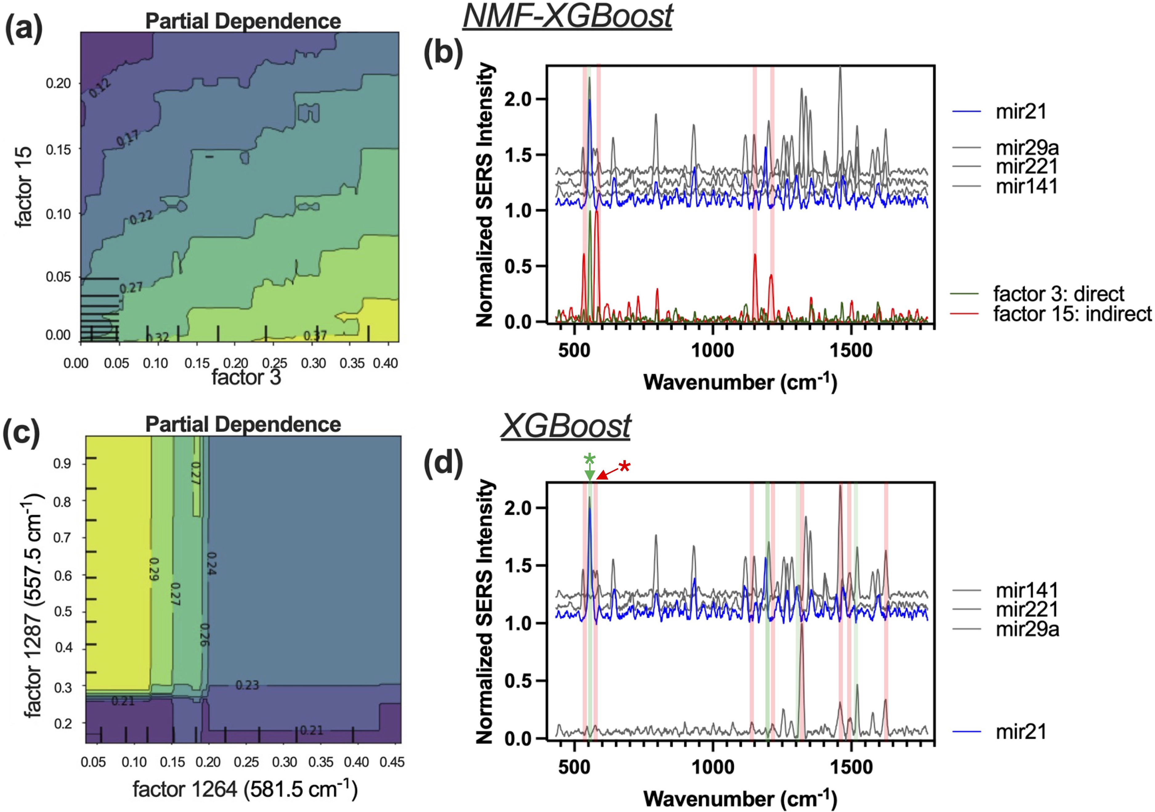
Non-negative matrix factorization-extreme gradient boosting (NMF-XGBoost): (a) PDP and (b) visualization of significant factors for the miRNA-21 target prediction. Panel (c) is a 2D partial dependence plot showing the effect of increasing NMF feature factors 3 and 15 (x- and y-axis, respectively) on the miRNA-21 prediction. (b) plots NMF features 3 (green) and 15 (red); reference spectra were offset by 0.1 and plotted with miRNA-21 reference in blue and all others in grey. Peak locations of NMF features 3 and 15 are highlighted in green and red, respectively, to show spectral locations with a direct relationship to miRNA-21 prediction in green and indirect relationship to miRNA-21 prediction in red. For XGBoost model alone, panel (c) is a 2D partial dependence plot showing the effect of increasing wavelength factors corresponding to 581.5 and 557.5 cm^–1 (x- and y-axis, respectively) on the miRNA-21 prediction; these wavelength factors are shown by red and green asterisks on (d); miRNA-21 reference is plotted in blue and all other references were offset and plotted in grey. Additional wavenumbers with significant partial dependence are highlighted: green for wavenumbers with a direct relationship to miRNA-21 prediction and red for wavenumber with an indirect relationship.

Clinical Samples Patient Selection and Collection

Clinical tissue samples were handled as previously described.¹³ Briefly, all experiments were approved by the Duke University Institutional Review Board (IRB Pro00001662). The Duke Gastrointestinal Tissue Repository enrolled patients who presented for endoscopic procedures and/or surgical resection of the esophagus at the Duke Department of Medicine Gastroenterology Clinic or Duke Surgery Division of Cardiovascular and Thoracic Surgery. Enrollment was also offered to patients who presented for Barrett's esophagus surveillance endoscopy, as well as those patients who received endoscopic ultrasound for endometrial cancer staging. Samples were snap frozen in liquid nitrogen, and then stored at −80 °C. De-identified and singly blinded samples were delivered to the operator performing the SERS iMS assay procedure. iMS assay was conducted as previously described. Briefly, 1 pM miR21-iMS was incubated with 100 ng of total small RNA extracted from tissue samples in 10 μL PBS–Tween-20 buffer at room temperature for 30 min. Then, 2 μL was transferred into a glass capillary tube and measured using the above system for three measurements, each with five accumulations of 30 s at a spectral range of 252.7–853.9 cm^–1.

Results and Discussion

Inverse Molecular Sentinel (iMS) for Multiplexed miRNA Sensing

Multiplexed iMS probes for miRNA panel miRNA-21, miRNA-29a, miRNA-221, and miRNA-141 with slight modification as previously described.¹³ As seen in Figure 1, the SERS signal is low when the placeholder is bound to the stem-loop and iMS probes are in the “OFF” configuration. The presence of a target miRNA displaces the placeholder and results in a stem-loop formation, bringing the SERS dye label in close proximity to the nanostar and resulting in an increase in the SERS signal when the iMS probes are in the “ON” configuration. SERS-based sensors operate by allowing the substance being measured (analyte) to interact directly with certain areas on the surface of the plasmonic metallic nanoparticle. This creates a response that follows a curve similar to the Langmuir isotherm, with the sensitivity of the sensor becoming very high at the ends of a specific concentration range. The range in which the target can be detected is determined by factors such as the number of particles and the amount of probe strands present. This behavior leads to a nonlinear response in the sensor when the target is present within certain concentration ranges, which has been observed in previous studies.¹³ Calibration curves and fit lines for each iMS “flavor” are shown in Figure 4.

Figure 4.

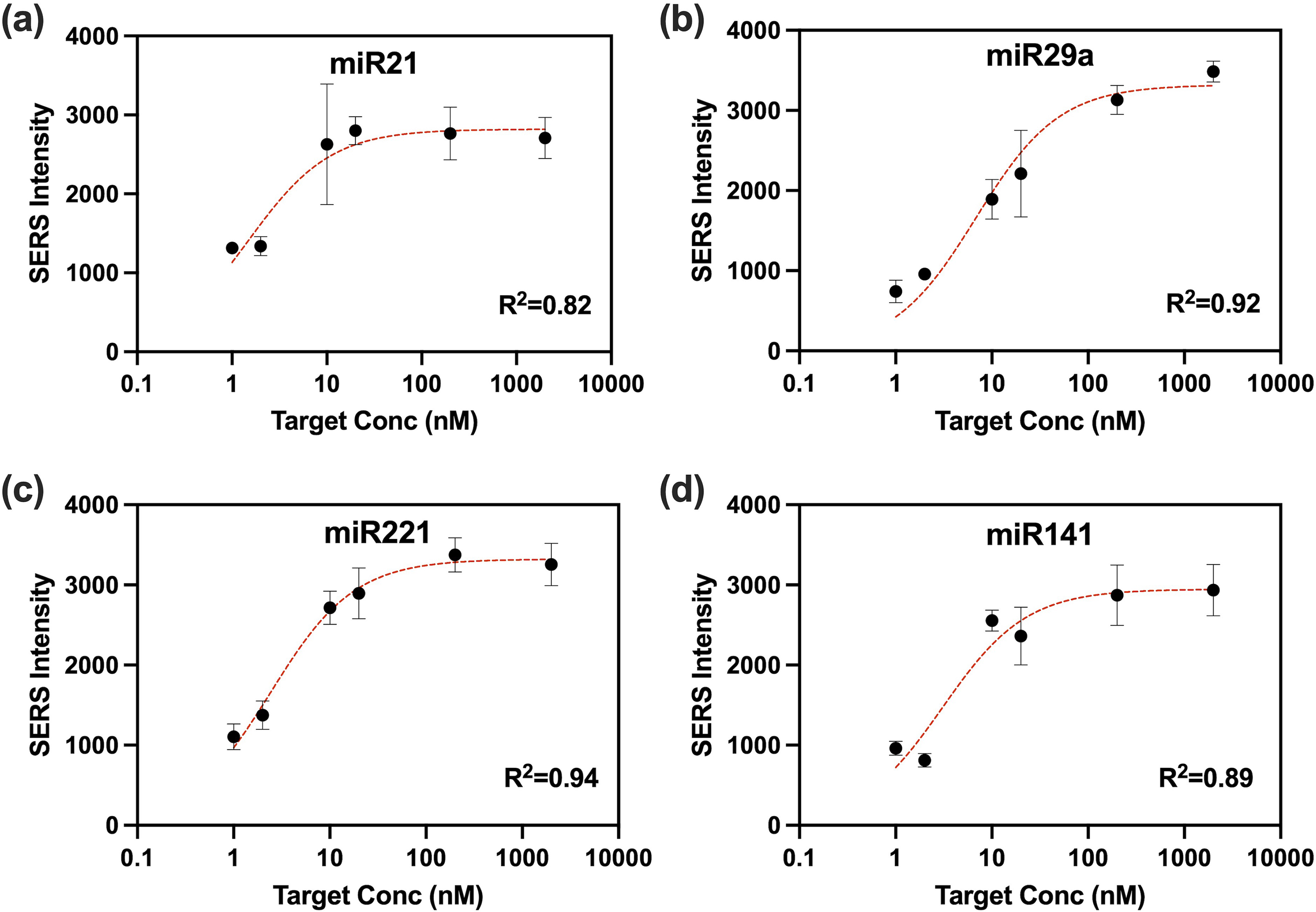
All four distinct iMS “flavors” were combined in a four-way multiplexed assay at different concentrations: miRNA-21 (5 pM), miRNA-141(25 pM), miRNA-221 (25 pM), and miRNA-29a (25 pM). The calibration data were curve fitted using a Langmuir-like surface saturation fit for each miRNA target in the four-way multiplexed iMS assay using synthetic DNA target for miRNA-21 (a) K_d=1.489±1.367; miRNA-29a (b) K_d=6.831±2.969; miRNA-221 (c) K_d=2.431±1.291; and miRNA-141 (d) K_d=3.083±1.340 nM.

Five-Fold CV

To evaluate the quality of model fit on the simulated training data, we performed five-fold CV on all six ML models using a training data set of n = 4000. Loss was determined by RMSE_label (Eq. 1) since the ground truth labels were known for this case. A one-way analysis of variance (ANOVA) on the RMSE_label for the six ML models revealed a highly significant p-value of 2.85 × 10^–11, which is much smaller than the alpha value of p = 0.05 (refer to Table S13, Supplemental Material). Furthermore, Tukey's post hoc testing demonstrated that SVR and CNN produced the best predictive performance in CV, with significantly lower RMSE_label compared to the other four models, but with no significant differences between them (Table S13, Supplemental Material). These results support previous findings.²⁷ In contrast, XGBoost showed the highest loss and performed significantly worse compared to most models. The NMF-based dimensionality reduced models exhibited similar performance, with no significant differences in RMSE_label between the three. The NMF-SVR and NMF-CNN models performed worse than their full-featured counterparts, which was expected since dimensionality reduction inevitably results in some loss of information. However, NMF-XGBoost outperformed XGBoost alone, potentially because (i) dimensionality reduction can help prevent overfitting, thus helping the model to generalize better to new data and (ii) dimensionality reduction can help handle multicollinearity, which is the case with multiplexed SERS spectra.

A one-way ANOVA on training time was conducted between all models, yielding a significant p-value of <2 × 10^–16, again much less than the alpha value, allowing for Tukey's post hoc testing (Table S13, Supplemental Material). Although CNN achieved one of the best performances, there is a tradeoff in training time; CNN needed significantly longer training times compared to all other models by at least one order of magnitude, followed by XGBoost and SVR. Dimensionality reduction decreased training time as expected due to decreased feature number, where NMF-SVR yielded the fastest training time, though it was not significant.

Validation on Multiplexed Test Sets

Model predictions were evaluated by RMSE_spectrum between projected, predicted spectra, and test spectra. For CNN, predicted and test spectra agree well (Figure S13, Supplemental Material) and the difference between the two spectra appears to be noise (Figure S14, Supplemental Material). CNN performed the most accurately over the entire test set with the lowest RMSE_spectrum of 8.86 × 10^–2 (Table II, second row). XGBoost alone had the second lowest RMSE_spectrum of 9.00 × 10^–2, followed by NMF-XGBoost and non-ML model SD, NMF-SVR, NMF-CNN, and SVR, which had the highest RMSE_spectrum. In the high S/N test subset, XGBoost alone performed best, followed by NMF-SVR, NMF-CNN, CNN, SVR, and finally SD (Table II, third row). However, in the low S/N test subset, SD performed the best, followed by XGBoost and CNN, NMF-XGBoost, NMF-SVR, NMF-CNN, and finally SVR.

Table II.

RMSE_label (Eq. 1) and fit times for five-fold validation for ML models without dimensionality reduction: SVR, XGBoost, and CNN, models with dimensionality reduction: NMF-SVR, NMF-XGBoost, and NMF-CNN.

	SVR	NMF-SVR	XGBoost	NMF-XGBoost	CNN	NMF-CNN	SD
Five-fold CVRMSE_label	6.73 × 10^–2 ± 1.55 × 10^–3	7.43 × 10^–2 ± 1.29 × 10^–3	7.77 × 10^–2 ± 1.21 × 10^–3	7.50 × 10^–2 ± 4.14 × 10^–4	6.98 × 10^–2 ± 2.10 × 10^–3	7.52 × 10^–2 ± 4.87 × 10^–4
Test set (n = 48) RMSE_spectrum	9.34 × 10^–2	9.10 × 10^–2	9.00 × 10^–2	9.02 × 10^–2	8.86 × 10^–2 ± 7.44 × 10^–5	9.19 × 10^–2 ± 1.18 × 10^–3	9.02 × 10^–2
High S/N test subset (n = 28) RMSE_spectrum	5.50 × 10^–2	5.31 × 10^–2	5.29 × 10^–2	5.71 × 10^–2	5.35 × 10^–2 ± 5.50 × 10^–5	5.33 × 10^–2 ± 1.00 × 10^–4	5.55 × 10^–2
Low S/N test subset (n = 20) RMSE_spectrum	1.29 × 10^–1	1.26 × 10^–1	1.24 × 10^–1	1.25 × 10^–1	1.24 × 10^–1 ± 1.51 × 10^–4	1.28 × 10^–1 ± 2.09 × 10^–3	1.23 × 10^–1
Training time	2.07 × 10¹ ± 9.39 × 10^–2	3.74 × 10^–1 ± 6.34 × 10^–2	2.19 × 10² ± 4.46 × 10²	3.66 ± 3.74 × 10^–1	1.14 × 10³ ± 1.23 × 10²	4.15 × 10¹ ± 2.00 × 10^–1

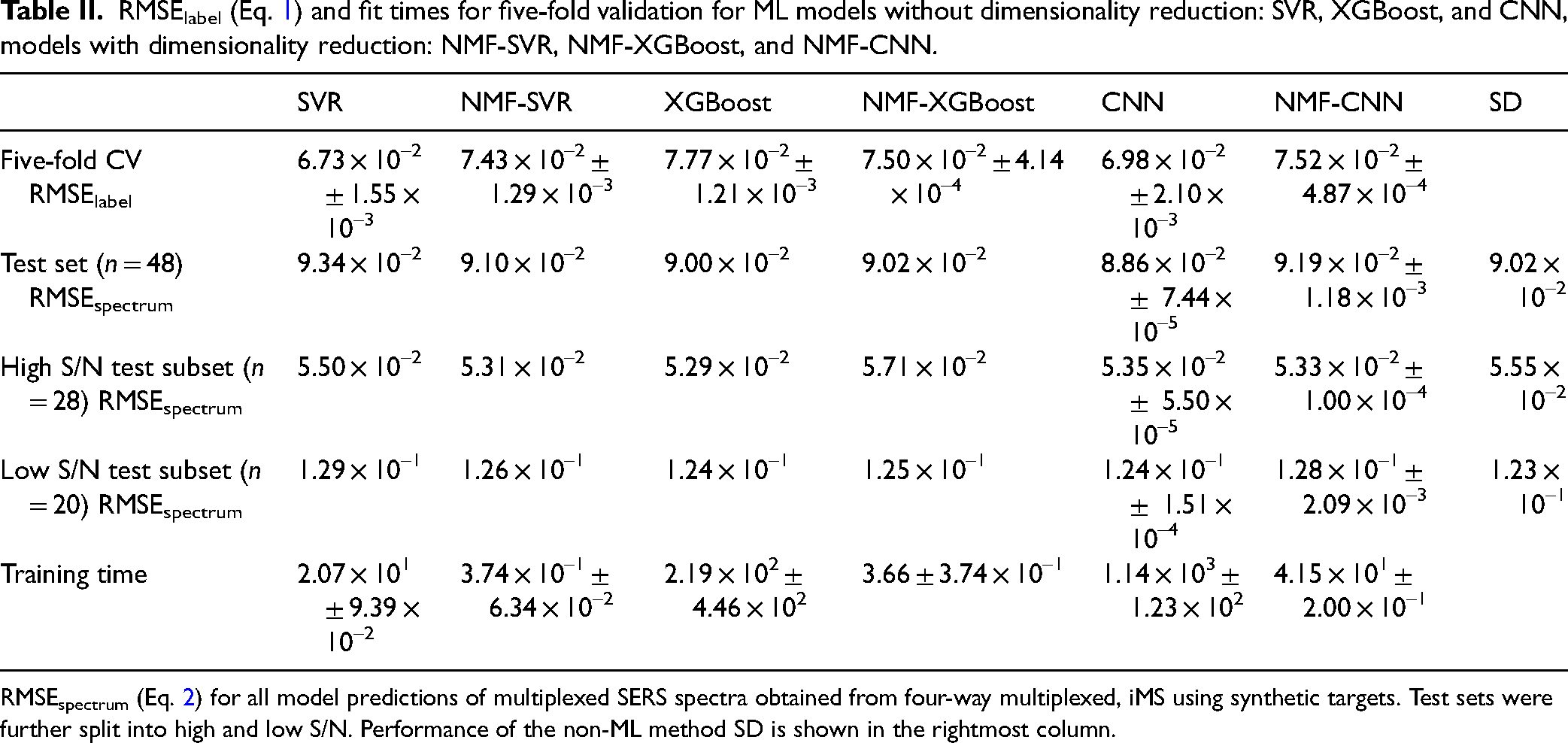
RMSE_spectrum (Eq. 2) for all model predictions of multiplexed SERS spectra obtained from four-way multiplexed, iMS using synthetic targets. Test sets were further split into high and low S/N. Performance of the non-ML method SD is shown in the rightmost column.

Although SVR alone performed the best in five-fold CV, it was amongst the worst performers for the overall test set as well as each subset. SVR's high RMSE_spectrum for the high S/N test subset may be due to overfitting while its high RMSE_spectrum for the low S/N test subset is congruent with previous results, where SVR was previously found to be less robust to noise.²⁷ While NMF dimensionality reduction improved performance for NMF-SVR, NMF resulted in worse performance compared to their counterparts for NMF-XGBoost and NMF-CNN. Interestingly, SD outperformed all ML models in the low S/N test subset but performed worse than all ML models in the high S/N test subset. This could potentially be because SD works by minimizing the RMSE_spectrum while ML models minimize RMSE_label during training. In extremely high noise spectra, RMSE_spectrum may not correlate well with RMSE_label. Thus, using RMSE_spectrum to evaluate prediction accuracy in high S/N data sets may be slightly skewed toward SD. Overall, model performance on the test set did not correlate with performance in a five-fold CV. Differences in model performance can be attributed to the experimental nature of the test set compared to CV, where the test set is a subset of the simulated training data.

Effect of Varying Training Set Size on Model Performance

The size of the training set was varied to investigate the relationship between training set size and model performance. As the training set size increased, RMSE_spectrum decreased overall for all models (Figure 5a), though improvements in accuracy slowed dramatically past n = 500 spectra. NMF-SVR and CNN-SVR showed more performance variability compared to other models, while CNN alone showed low variability and maintained the lowest RMSE_spectrum in all cases. XGBoost alone and NMF-XGBoost performed similarly in all cases and had the second lowest RMSE_spectrum where training set size n > 100. NMF-CNN and NMF-SVR SVR maintained the highest RMSE_spectrum in most cases.

Figure 5.

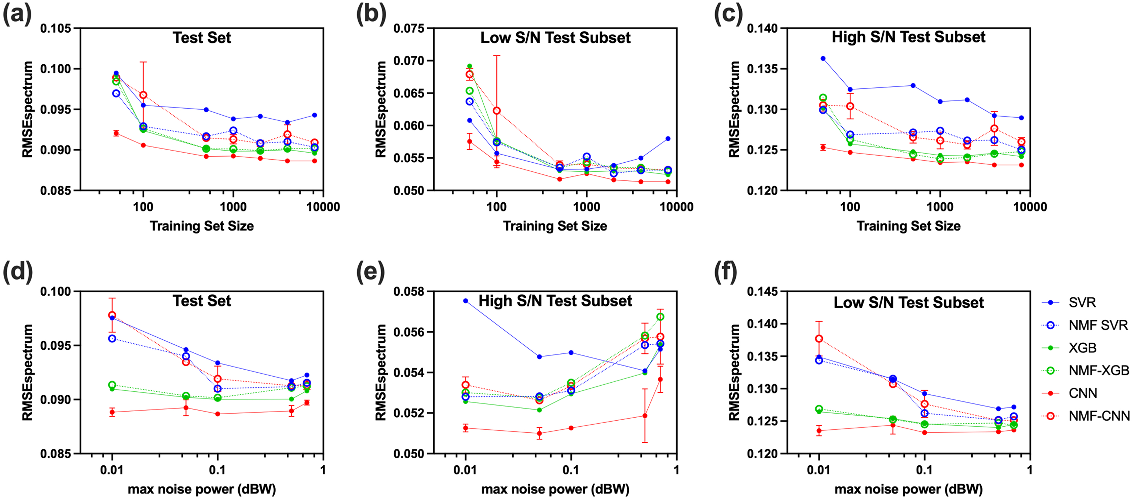
RMSE_spectrum (Eq. 2) performance of n=3 CNN, SVR, and XGBoost, on the whole test set (a) high S/N test set (c), and low S/N test set (b) are plotted as filled circular markers for training sets of size n=50, 100, 500, 1000, 2000, 4000, and 8000 (70% training, 30% validation) on a semi-log plot. RMSE_spectrum performance of n=3 NMF-CNN, NMF-SVR, and NMF-XGBoost, on the whole test set (a), high S/N test set (b), and low S/N test set (c) are plotted as hollow circular markers for above-mentioned training sets sizes (70% training, 30% validation) on a semi-log plot. RMSE_spectrum performance (Eq. 2) of n=3 CNN, n=3 NMF-CNN, SVR, NMF-SVR, XGBoost, and NMF-XGBoost on the entire test set (d), high S/N subset (e), and low S/N subset (f) for training sets of varying maximum noise added during simulation. Performance of models without dimensionality reduction are plotted as filled circular markers and performance of models with NMF dimensionality reduction are plotted as hollow circular markers on a semi-log plot.

The RMSE_spectrum behaved differently between the high and low S/N test subsets. With the high S/N test subset, trends between and within models are very similar to overall performance (Figure 5c). The largest difference was that SVR had the highest RMSE_spectrum with a larger gap between SVR and the other models. With the low S/N test subset, RMSE_spectrum decreased more dramatically with increasing training set size for all models. All models except SVR continued to improve in accuracy with increasing training set size. SVR, however, achieved the lowest RMSE_spectrum at n = 500 and had an increasing RMSE_spectrum as the training set size increased past n = 500. This again suggests SVR overfitting.

Although CNN performed with the highest accuracy, it pays with the tradeoff of the longest training time. NMF-CNN has the second longest training time when n < 4000. CNN training times can be reduced by changing CNN architecture, but this may be at the cost of accuracy. There is a tradeoff between training time and computational power versus accuracy. For small training size n < 4000, SVR and NMF-SVR are quite fast compared to other models. However, because the hyperspace takes every training spectrum into consideration, training time increases exponentially, much faster than all other models. Combined with overfitting tendencies, SVR is unsuitable for large training sets.

Effect of Varying Added Noise on Model Performance

During the data simulation process, Gaussian noise was added with a power selected randomly within a given range. It is important to investigate how much noise should be added to improve the model's robustness to noise without compromising accuracy in high S/N spectra. To investigate the effect of maximum noise power added on the tradeoff between robustness and accuracy, the maximum noise power was changed while keeping the minimum noise power within the power range constant. The low S/N test subset contributes more to the effect of max noise power on the overall test set performance since noise inherently increases the RMSE_spectrum (Figures 5d and 5f), thus contributing more to the total loss. Therefore, it is important to look at the high and low S/N subsets separately to determine the behavior in either case.

In the high S/N test subset, SVR, NMF-SVR, XGBoost, NMF-XGBoost, and NMF-CNN showed a decrease in accuracy with an increase in max noise power, which is expected as lower noise data sets are more representative of the high S/N test subset. On the other hand, in the low S/N test subset, increasing the max noise power generally improved prediction accuracy for the same reason. The effect of noise level on the performance in the overall test set is a combination of these two trends, resulting in a general trend of decreasing then increasing loss as max noise power increases. SVR, NMF-SVR, and NMF-CNN had the strongest dependence on max noise power, with the most rapid decrease in RMSE_spectrum as max noise power increased to 0.1 dB. As per previous findings,²⁷ SVR is prone to overfitting, which is evident in the high S/N subset, where the SVR loss shows an opposite trend of decreasing RMSE_spectrum with increasing max noise power in the range [0.01–0.5]. This is because increasing the added noise in the training set decreases overfitting in SVR, resulting in better performance. On the other hand, NMF-SVR displayed the opposite trend to SVR in the high S/N subset, where lower max noise added resulted in more accurate predictions, indicating that adding dimensionality reduction before SVR reduced overfitting.

Convolutional neural networks (CNNs) did not exhibit a strong dependence on the added max noise power, which can be attributed to the lack of a discernible trend in the low S/N test subset, as depicted in Figure 5f. This shows that CNN is highly robust to noise, even during training, due to the convolutional nature of the model, which agrees with previous findings.²⁷ Unlike CNN alone, NMF-CNN showed strong dependence on training noise, suggesting that dimensionality reduction decreased robustness for CNN. The performance of XGBoost and NMF-XGBoost also did not exhibit strong dependence on added max power. In the high S/N test subset, both models displayed increased loss with increasing max noise power, where NMF-XGBoost performed worse for all conditions compared to XGBoost. However, in the low S/N test subset, both models performed similarly and had a slight downward trend in RMSE_spectrum with increasing max noise power, suggesting that both XGBoost and NMF-XGBoost are quite robust to high noise spectra and are not very affected by the level of noise during training.

Extreme Gradient Boost Model Interpretation

Partial dependence plots (PDPs) can visualize the associations between selected features on interest and target response, which can be used to understand which features affect the predictions. In NMF-XGBoost, each feature is an NMF component. The 2D partial dependence plot of two significant features for the miRNA-21 target prediction in NMF-XGBoost is shown in Figure 3a, which shows that as factor 3 increases, the predicted miRNA-21 component also increases and when factor 15 increases, the predicted miRNA-21 component decreases. The factor 3 NMF component has one main peak at 557.5 cm^–1 (Figure 3b, green trace), which corresponds to the main miRNA-21-Cy5 peak. So, the NMF-XGBoost is using the main 557 cm^–1 peak to predict the miRNA-21 contribution with a direct relationship. The factor 15 NMF component has 4 main peaks (Figure 3b, red trace). Two of these peaks, located at 552.3 and 577.3 cm^–1, flank the main 557 cm^–1 peak and delineate the edges of the main sharp peak. From the reference plot in grey, we see that there are peaks from other target references on either side of the main 557 cm^–1 peak. The NMF-XGBoost model predicts higher miRNA-21 contribution when the spectral values on either side of the main 557 cm^–1 peak decrease, resulting in a sharper peak. Thus, the NMF-XGBoost model predicts higher miRNA-21 contribution when the 557 cm^–1 peak increases and becomes sharper and more defined.

In the XGBoost alone model, each feature corresponds to a single spectral value. The 2D PDP of two significant spectral values are shown in Figure 3c. An increase in factor 1287, which corresponds to the spectral value of the main miRNA-21-Cy5 peak at 557 cm^–1 (Figure 3d, green asterisk), results in an increase in the prediction of miRNA-21 contribution. An increase in factor 1264, corresponding to the spectral value of 581.5 cm^–1 (Figure 3d, red asterisk), located at the right end of the main 557 cm^–1 peak, results in a decrease in the prediction of miRNA-21 contribution. Spectral locations of additional significant factors with direct and indirect relationships to the miRNA-21 target prediction are shown in green and red, respectively. Significant direct spectral locations correspond to a main unique peak at 557 cm^–1. Significant indirect spectral locations are generally located at the edges of miRNA-21 peaks where references have large peaks. Compared to the PDP in the NMF-XGBoost model, the PDP in the XGBoost model is less linear/smooth due to the variability of a single spectral value, especially with noisy and complex data.

The CNN can be interpreted using the gradient class activation map³⁹ method to produce saliency maps that highlight the spectral regions most responsible for target predictions (Figure S17, Supplemental Material). Interpretation plots based on PDPs for NMF-SVR, SVR, NMF-XGBoost, and XGBoost are shown in Figures S18–S21 (Supplemental Material).

Application to Clinical Data

All seven analysis methods were applied to the clinical data. All ML models were trained with multiplexed training spectra in the smaller spectral range. The reference spectra of miRNA-141 and miRNA-29a were inverted in the range²⁷ because all spectral features for the two corresponding dyes were outside of the acquired spectral range. However, this approach still demonstrates the performance of these ML models on clinical spectra. NMF-XGBoost achieved the lowest RMSE_spectrum, followed by SD, NMF-SVR, XGBoost, SVR, CNN, and lastly NMF-CNN (Table III). It is noteworthy that this performance is different on the multiplexed test set above. This can be expected due to the limited spectral range acquired and low S/N of the clinical assay spectra compared to the larger differential thermal analysis set used in the test sets. Prediction accuracy was also evaluated by RMSE_label since the ground truth label is known and determined by the AUC of the spectrum under the main 557 cm^–1 peak. Here NMF-CNN achieved the lowest RMSE_label of 9.68 × 10^–2, followed by CNN, NMF-SVR, NMF-XGBoost, SVR, XGBoost, and lastly, SD. The two-loss metrics RMSE_spectrum and RMSE_label did not correlate well with each other, potentially due to the low S/N nature of the clinical assay spectrum. In this case, RMSE_spectrum is dominated by noise, and inaccurate predictions which overfit the noise would yield a lower RMSE_spectrum but more inaccurate RMSE_label. Therefore, RMSE_label is a better indicator of prediction accuracy, while RMSE_spectrum in conjunction with RMSE_label can indicate overfitting to noise.

Table III.

First row shows the RMSE_spectrum performance (Eq. 2) of non-ML model SD, ML models with and without dimensionality reduction on the clinical spectra. The second row shows the RMSE_label performance (Eq. 1) of all models on clinical spectra. Ground truth labels were calculated from clinical spectra AUC.

	SD	CNN	NMF-CNN	SVR	NMF-SVR	XGBoost	NMF-XGBoost
Clinical RMSE_spectrum	1.720 × 10^–1	1.740 × 10^–1	1.741 × 10^–1	1.733 × 10^–1	1.723 × 10^–1	1.726 × 10^–1	1.717 × 10^–1
Clinical RMSE_label	3.51 × 10^–1	1.01 × 10^–1	9.68 × 10^–2	1.90 × 10^–1	1.36 × 10^–1	1.94 × 10^–1	1.45 × 10^–1

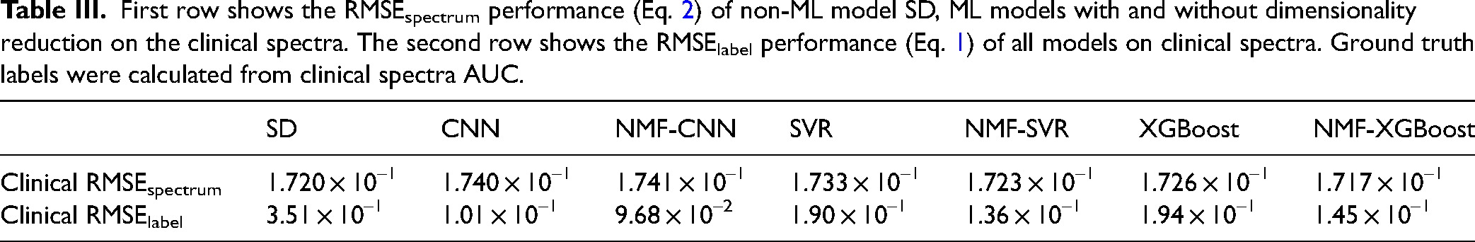
Spectral decomposition (SD) outperformed five out of six ML models in RMSE_spectrum, however, it had the highest RMSE_label. Because SD minimizes RMSE_spectrum, it overfits noise and yields an inaccurate prediction. NMF-CNN and CNN produced the most accurate predictions, with the lowest RMSE_label, but had the highest RMSE_spectrum, indicating accurate predictions without overfitting to noise or training set. In all cases, NMF models outperformed their full-featured counterparts in the RMSE_label, suggesting that dimensionality reduction could improve generalizability from the simulated training set to the clinical assay spectra by helping to deal with multicollinearity. Notably, there are limitations to this analysis as it only demonstrates the case of a single target in a multiplexed assay.

Clinical spectra were previously evaluated by the (AUC of the 557 cm^–1 main peak for miRNA-21-Cy5. Thus, model predictions were correlated with AUC. NMF-CNN and CNN achieved the highest R² value (Figure 6a), which is consistent with RMSE_label. SVR achieved a higher R² value than NMF-SVR, but lower than both CNN and NMF-CNN (Figure 6b). XGBoost had a better fit than NMF-XGBoost and worse than all other ML models (Figure 6c). All ML model predictions had a greater correlation with AUC than SD.

Figure 6.

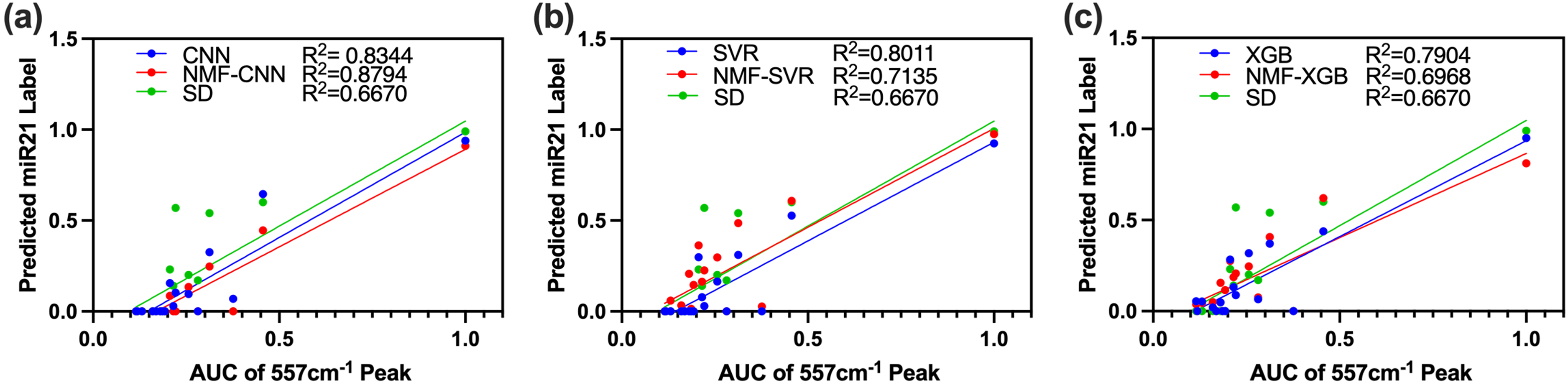
Predicted miRNA-21 labels by (a) CNN and NMF-CNN, (b) SVR and NMF-SVR, and (c) XGBoost and NMF-XGBoost plotted versus AUC of the characteristic peak at 557 cm^–1 of clinical test spectra. Clinical data was obtained from esophageal tissues using single plex miRNA-21-Cy7 probes. Models were trained on simulated multiplexed data using references as previously discussed. miRNA-21-Cy7 references were obtained from the same iMS particles as used in clinical study. Reference spectra were obtained using 1 or 4 nM synthetic miRNA-21 RNA as an average of 10 spectra.

Comparative Analysis of ML Models

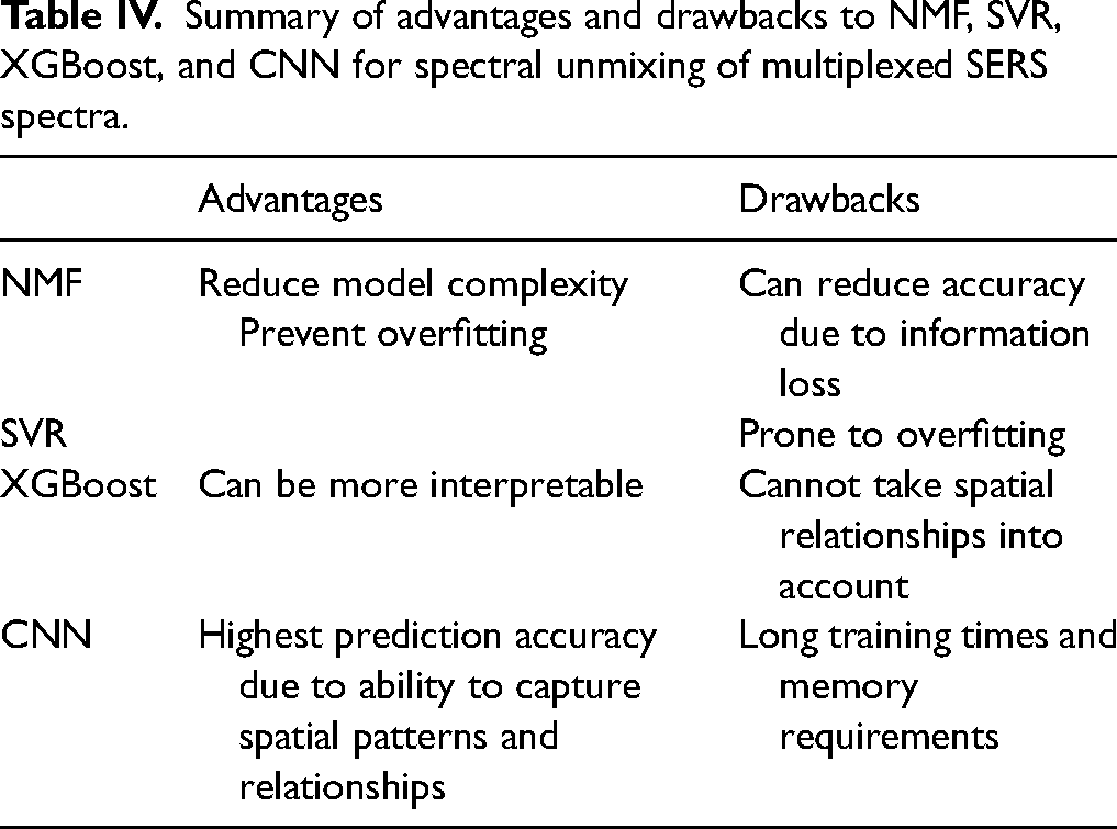
Overall, NMF dimensionality reduction reduces model complexity and can prevent overfitting for complex ML models at the expense of some information loss. NMF can be used with a variety of ML models. Here we investigated SVR, XGBoost, and CNN (Table IV). SVR performed well in five-fold CV but did not generalize to experimentally acquired multiplexed spectra due to overfitting. XGBoost performed relatively accurately and can be more interpretable than CNN but cannot outperform CNN because it cannot retain spatial relationships. Finally, CNN achieves the highest accuracy predictions due to its convolutional nature but requires the most memory, computing power, and training times. It is important to choose the model based on the application.

Table IV.

Summary of advantages and drawbacks to NMF, SVR, XGBoost, and CNN for spectral unmixing of multiplexed SERS spectra.

	Advantages	Drawbacks
NMF	Reduce model complexityPrevent overfitting	Can reduce accuracy due to information loss
SVR		Prone to overfitting
XGBoost	Can be more interpretable	Cannot take spatial relationships into account
CNN	Highest prediction accuracy due to ability to capture spatial patterns and relationships	Long training times and memory requirements

Conclusion

In conclusion, CNN, SVR, and XGBoost alone and combined with NMF dimensionality reduction are powerful techniques that can improve the spectral unmixing of multiplexed SERS spectra. NMF can reduce overfitting and decrease training time and computational power requirements while helping handle collinearity and improving model interpretability. On the other hand, SVR can be prone to overfitting, which can compromise its accuracy and generalization capabilities. Additionally, NMF can be used to significantly reduce the number of model parameters required for a given architecture, making it an efficient and effective technique for simplifying models to save computational time and memory. Overall, the use of NMF and other dimensionality reduction techniques in conjunction with ML algorithms such as CNN can lead to improved model performance and better predictions in SERS spectral unmixing.

Supplemental Material

sj-docx-1-asp-10.1177_00037028231209053 - Supplemental material for Surface-Enhanced Raman Spectroscopy-Based Detection of Micro-RNA Biomarkers for Biomedical Diagnosis Using a Comparative Study of Interpretable Machine Learning Algorithms

Supplemental material, sj-docx-1-asp-10.1177_00037028231209053 for Surface-Enhanced Raman Spectroscopy-Based Detection of Micro-RNA Biomarkers for Biomedical Diagnosis Using a Comparative Study of Interpretable Machine Learning Algorithms by Joy Q. Li, Hsin Neng-Wang, Aidan J. Canning, Alejandro Gaona, Bridget M. Crawford, Katherine S. Garman and Tuan Vo-Dinh in Applied Spectroscopy

Footnotes

Declaration of Conflicting Interests

The authors declared no potential conflicts of interest with respect to the research, authorship, and/or publication of this article.

Funding

The authors disclosed receipt of the following financial support for the research, authorship, and/or publication of this article: This study is supported by the National Institute of General Medical Sciences, National Institute of Dental and Craniofacial Research (grant nos. NIDCR-1R01DE030455-01A1 and NIGMS-R01GM135486). Joy Li received support from the National Defense Science and Engineering Graduate Fellowship (Fellow ID: 00007902).

ORCID iD

Tuan Vo-Dinh

Supplemental Material

All supplemental material mentioned in the text is available in the online version of the journal.

References

Vo-Dinh

Begun

M.Y.K.G.M.

Moody

R.L.

. “Surface-Enhanced Raman Spectrometry for Trace Organic Analysis”. Anal. Chem. 1984. 56(9): 1667–1670. 10.1021/ac00273a029

Vo-Dinh

. “Surface-Enhanced Raman Spectroscopy Using Metallic Nanostructures”. TrAC, Trends Anal. Chem. 1998. 17(8–9): 557–582. 10.1016/S0165-9936(98)00069-7

Langer

Jimenez de Aberasturi

Aizpurua

Alvarez-Puebla

R.A.

, et al. “Present and Future of Surface-Enhanced Raman Scattering”. ACS Nano. 2020. 14(1): 28–117. 10.1021/acsnano.9b04224

Cupil-Garcia

Strobbia

Crawford

B.M.

Wang

H.-N.

, et al. “Plasmonic Nanoplatforms: From Surface-Enhanced Raman Scattering Sensing to Biomedical Applications”. J. Raman Spectrosc. 2021. 52(2): 541–553. 10.1002/jrs.6056

Eremina

O.E.

Czaja

A.T.

Fernando

Aron

, et al. “Expanding the Multiplexing Capabilities of Raman Imaging to Reveal Highly Specific Molecular Expression and Enable Spatial Profiling”. ACS Nano. 2022. 16(7): 10341–10353. 10.1021/acsnano.2c00353

Thrift

W.J.

Ragan

. “Quantification of Analyte Concentration in the Single Molecule Regime Using Convolutional Neural Networks”. Anal. Chem. 2019. 91(21): 13337–13342. 10.1021/acs.analchem.9b03599

Alak

A.M.

Vo-Dinh

. “Silver Coated Fumed Silica as a Substrate Material for Surface Enhanced Raman Scattering”. Anal. Chem. 1989. 61(7): 656–660. 10.1021/ac00182a004

Volkan

Stokes

D.L.

Vo-Dinh

. “Surface-Enhanced Raman of Dopamine and Neurotransmitters Using Sol-Gel Substrates and Polymer-Coated Fiber-Optic Probes”. Appl. Spectrosc. 2000. 54(12): 1842–1848. 10.1366/0003702001948952

Yan

Wabuyele

M.B.

Griffin

G.D.

Vass

A.A.

Vo-Dinh

. “Surface-Enhanced Raman Scattering Detection of Chemical and Biological Agent Simulants”. IEEE Sens. J. 2005. 5(4): 665–670. 10.1109/JSEN.2005.850993

10.

Ngo

H.T.

Gandra

Fales

A.M.

Taylor

S.M.

Vo-Dinh

. “Sensitive DNA Detection and SNP Discrimination Using Ultrabright SERS Nanorattles and Magnetic Beads for Malaria Diagnostics”. Biosens. Bioelectron. 2016. 81: 8–14. 10.1016/j.bios.2016.01.073

11.

Wang

H.N.

Fales

A.M.

Zaas

A.K.

Woods

C.W.

, et al. “Surface-Enhanced Raman Scattering Molecular Sentinel Nanoprobes for Viral Infection Diagnostics”. Anal. Chim. Acta. 2013. 786: 153–158. 10.1016/j.aca.2013.05.017

12.

Dukes

P.V.

Strobbia

Ngo

H.T.

Odion

R.A.

, et al. “Plasmonic Assay for Amplification-Free Cancer Biomarkers Detection in Clinical Tissue Samples”. Anal. Chim. Acta. 2020. 1139: 111–118. 10.1016/j.aca.2020.09.003

13.

Crawford

B.M.

Wang

H.N.

Stolarchuk

von Furstenberg

R.J.

, et al. “Plasmonic Nanobiosensors for Detection of Microrna Cancer Biomarkers in Clinical Samples”. Analyst. 2020. 145(13): 4587–4594. 10.1039/D0AN00193G

14.

Canning

A.J.

Chen

J.Q.

Jeck

W.R.

, et al. “MiRNA Probe Integrated Biosensor Platform Using Bimetallic Nanostars for Amplification-Free Multiplexed Detection of Circulating Colorectal Cancer Biomarkers in Clinical Samples”. Biosens. Bioelectron. 2023. 220: 114855. 10.1016/j.bios.2022.114855s

15.

Condrat

C.E.

Thompson

D.C.

Barbu

M.G.

Bugnar

O.L.

, et al. “MiRNAs as Biomarkers in Disease: Latest Findings Regarding Their Role in Diagnosis and Prognosis”. Cells. 2020. 9(2): 276. 10.3390/cells9020276.

16.

Inokuchi

Ochiya

Matsuzaki

. “Extracellular miRNAs for the Management of Barrett's Esophagus and Esophageal Adenocarcinoma: A Systematic Review”. J. Clin. Med. 2020. 10(1): 117. 10.3390/jcm10010117

17.

Wang

Rufo

Chen

, et al. “Acoustofluidic Salivary Exosome Isolation: A Liquid Biopsy Compatible Approach for Human Papillomavirus-Associated Oropharyngeal Cancer Detection”. J. Mol. Diagn. 2020. 22(1): 50–59. 10.1016/j.jmoldx.2019.08.004

18.

Zhou

S.-S.

Jin

J.-P.

Wang

J.-Q.

Zhang

Z.-G.

, et al. “MiRNAs in Cardiovascular Diseases: Potential Biomarkers, Therapeutic Targets, and Challenges”. Acta Pharmacol. Sin. 2018. 39(7): 1073–1084. 10.1038/aps.2018.30

19.

Wang

Zhang

. “Circulating Exosomal miRNA as Diagnostic Biomarkers of Neurodegenerative Diseases”. Front. Mol. Neurosci. 2020. 13. 10.3389/fnmol.2020.00053

20.

Guerrini

Alvarez-Puebla

R.A.

. “Surface-Enhanced Raman Spectroscopy in Cancer Diagnosis, Prognosis, and Monitoring”. Cancers 2019. 11(6): 748. 10.3390/cancers11060748

21.

Fales

A.M.

Yuan

Vo-Dinh

. “Development of Hybrid Silver-Coated Gold Nanostars for Nonaggregated Surface-Enhanced Raman Scattering”. J. Phys. Chem. C. 2014. 118(7): 3708–3715. 10.1021/jp4091393

22.

Garman

K.S.

Owzar

Hauser

E.R.

Westfall

, et al. “MicroRNA Expression Differentiates Squamous Epithelium from Barrett's Esophagus and Esophageal Cancer”. Dig. Dis. Sci. 2013. 58(11): 3178–3188. 10.1007/s10620-013-2806-7

23.

Yang

Zhou

Xiang

Chen

. “Serum microRNAs: A New Diagnostic Method for Colorectal Cancer”. Biomed. Rep. 2013. 1(4): 495–498. 10.3892/br.2013.109

24.

Rapado-González

Ó.

Álvarez-Castro

López-López

Iglesias-Canle

, et al. “Circulating microRNAs as Promising Biomarkers in Colorectal Cancer”. Cancers. 2019. 11(7): 898. 10.3390/cancers11070898

25.

Ding

Sun

Liu

Jiang

Q.-Y.

. et al. “SERS-Based Biosensors Combined with Machine Learning for Medical Application”. ChemistryOpen. 2023. 12(1): e202200192. 10.1002/open.202200192

26.

Kobayashi

Kaneko

Tamaki

Kiguchi

, et al. “Principal Component Analysis of Surface-Enhanced Raman Scattering Spectra Revealing Isomer-Dependent Electron Transport in Spiropyran Molecular Junctions: Implications for Nanoscale Molecular Electronics”. ACS Omega. 2022. 7(6): 5578–5583. 10.1021/acsomega.1c07105

27.

J.Q.

Dukes

P.V.

Lee

Sarkis

Vo-Dinh

. “Machine Learning Using Convolutional Neural Networks for SERS Analysis of Biomarkers in Medical Diagnostics”. J. Raman Spectrosc. 2022. 53(12): 2044. 10.1002/jrs.6447.

28.

Chen

Luo

, et al. “Raman Spectroscopy Combined with a Support Vector Machine Algorithm as a Diagnostic Technique for Primary Sjögren’s Syndrome”. Sci. Rep. 2023. 13(1): 5137. 10.1038/s41598-023-29943-9

29.

Sellers

Kwon

J.S.-I.

H.-J.

. “Integration of Surface-Enhanced Raman Spectroscopy (SERS) and Machine Learning Tools for Coffee Beverage Classification”. Digital Chem. Eng. 2022. 3: 100020. 10.1016/j.dche.2022.100020

30.

Rojalin

Antonio

Kulkarni

Carney

R.P.

. “Machine Learning-Assisted Sampling of SERS Substrates Improves Data Collection Efficiency”. Appl. Spectrosc. 2022. 76(4): 485-495. 10.1177/00037028211034543.

31.

Gao

Zhou

Liu

Guan

, et al. “Machine Learning Prediction of Lignin Content in Poplar with Raman Spectroscopy”. Bioresour. Technol. 2022. 348: 126812. 10.1016/j.biortech.2022.126812

32.

Liu

Xue

Yang

Zhang

. “Rapid Identification and Drug Resistance Screening of Respiratory Pathogens Based on Single-Cell Raman Spectroscopy”. Front Microbiol. 2023. 14: 1065173. 10.3389/fmicb.2023.1065173

33.

Erzina

Trelin

Guselnikova

Dvorankova

, et al. “Precise Cancer Detection via the Combination of Functionalized SERS Surfaces and Convolutional Neural Network with Independent Inputs”. Sens. Actuators, B. 2020. 308: 127660. 10.1016/j.snb.2020.127660

34.

Zhu

Sharma

A.S.

, et al. “Rapid On-Site Identification of Pesticide Residues in Tea by One-Dimensional Convolutional Neural Network Coupled with Surface-Enhanced Raman Scattering”. Spectrochim. Acta, Part A. 2021. 246: 118994. 10.1016/j.saa.2020.118994

35.

Kazemzadeh

Hisey

C.L.

Zargar-Shoshtari

Broderick

N.G.R.

. “Deep Convolutional Neural Networks as a Unified Solution for Raman Spectroscopy-Based Classification in Biomedical Applications”. Opt. Commun. 2022. 510: 127977. 10.1016/j.optcom.2022.127977

36.

Lutz

B.R.

Dentinger

C.E.

Nguyen

L.N.

Sun

, et al. “Spectral Analysis of Multiplex Raman Probe Signatures”. ACS Nano. 2008. 2(11): 2306–2314. 10.1021/nn800243g

37.

Wang

H.N.

Crawford

B.M.

Fales

A.M.

Bowie

M.L.

, et al. “Multiplexed Detection of MicroRNA Biomarkers Using SERS-Based Inverse Molecular Sentinel (iMS) Nanoprobes”. J. Phys. Chem. C. 2016. 120(37): 21047–21050. 10.1021/acs.jpcc.6b03299

38.

Zhang

Servos

M.R.

Liu

. “Instantaneous and Quantitative Functionalization of Gold Nanoparticles with Thiolated DNA Using a pH-Assisted and Surfactant-Free Route”. J. Am. Chem. Soc. 2012. 134(17): 7266–7269. 10.1021/ja3014055

39.

Selvaraju

R.R.

Cogswell

Das

Vedantam

, et al. “Grad-CAM: Visual Explanations from Deep Networks via Gradient-Based Localization”. In: 2017 IEEE International Conference on Computer Vision (ICCV). Venice, Italy: 22–29 October 2017. Pp. 618–626. 10.1109/ICCV.2017.74

Supplementary Material

Please find the following supplemental material available below.

For Open Access articles published under a Creative Commons License, all supplemental material carries the same license as the article it is associated with.

For non-Open Access articles published, all supplemental material carries a non-exclusive license, and permission requests for re-use of supplemental material or any part of supplemental material shall be sent directly to the copyright owner as specified in the copyright notice associated with the article.

0.00 MB

6.14 MB