Sage Journals: Discover world-class research

Abstract

Disparities in state and local government spending are key drivers of spatial inequality in social outcomes, including economic mobility. Yet beyond spending levels, the fiscal centralization of state and local governments—that is, the relative role of higher- versus lower-level governments in taxing, spending, and public employment—also differs substantially, traceable to place-specific founding circumstances and path dependent historical trajectories. In this study, we ask, in more centralized fiscal systems, is there less spatial inequality in the economic mobility outcomes of low-income children? To answer this, we construct a novel Fiscal Centralization Index for each state and each county using data from the U.S. Census of Governments. We then use place-based estimates of intergenerational economic mobility, provided by Opportunity Insights, to measure cross-census-tract variation in the mobility outcomes of children within each state and each county. We find that more centralized fiscal structures exhibit less spatial inequality in the economic mobility outcomes of low-income children, and this is driven by improving outcomes in lower-performing census tracts. Our findings motivate the fiscal sociology of place as a framework for revealing how historically conditioned fiscal systems are implicated in the production of place-based inequalities, with the potential to generate new insights and policy interventions.

Keywords

economic mobility inequality place government fiscal policy

A map displaying the intergenerational economic mobility outcomes of low-income children in the United States affirms an emergent social science consensus: place matters. Where individuals live, and where they grow up, has a causal effect on outcomes over the life course, from educational achievement and attainment to labor market performance and household formation to the likelihood of incarceration and early mortality (Chetty, Hendren, and Katz 2016; Edin, Shaefer, and Nelson 2023; Gieryn 2000; Lobao 2004; Michener 2018; Montez et al. 2020; Reardon and Owens 2014; Sampson 2019; Sharkey 2008; Sharkey and Faber 2014). What accounts for this powerful effect of place? Beyond concentrated disadvantage (Massey and Denton 1993; Wilson 1987, 1997), scholars often point to differences in state and local government policy—including expenditures on education, health, and social welfare—as a primary driver of place-based differences in social outcomes (see, e.g., Lobao 2016; Lobao et al. 2012; Massey 1990). Equitizing local public sectors is therefore key to mitigating the effect of place on life chances.

The United States, like other federal systems, has three tiers of government—federal, state, and local—each with overlapping responsibilities for financing and instantiating the public sector. In the U.S. context, the local tier is further fragmented into myriad, semi-nested agglomerations of county, municipal, and district governments, each with specific fiscal roles, authorities, and obligations. Taxes can only be levied on income, property, and consumption within jurisdictional borders, so the fiscal capacity of subnational (i.e., state and local) governments differs widely—and is a primary driver of disparities in government spending (Gordon, Auxier, and Iselin 2016). In such federated fiscal systems, there are two ways to offset differences in local fiscal capacity and the resulting inequities in government services (see Buchanan 1950; Highsmith 2019, 2020; Liscow 2017). The first is through fiscal redistribution, whereby the central or higher-level government provides revenue transfers to lower governments to offset disparities in taxable wealth and social need. The second is through fiscal centralization, whereby the central or higher-level government performs the bulk of fiscal policy-making and service delivery, rendering lower-level governments less consequential.

The United States is a notable outlier on fiscal redistribution: it is the only rich federal democracy without an explicit policy to equalize fiscal resources across states (Béland and Lecours 2014). Governments in wealthy states such as New York, California, and Massachusetts routinely receive more dollars per capita from the federal government than do governments in poorer states like Alabama or Kansas (McCabe 2017; Stark 2009). Within states, however, there is typically some effort to equalize resources across local governments, particularly to reduce inequities in K–12 education spending funded via local property taxes (Hoxby 2001). In the past three decades, 26 states adopted more than 67 school finance reforms, most expressly designed to redistribute resources to poorer districts (Shores, Candeleria, and Kabourek 2019). A growing body of research finds redistributing public funds to poorer places improves social outcomes; for example, Biasi (2023) finds higher K–12 spending induced by school finance reforms improved the upward mobility outcomes of low-income children residing in poorer school districts (see also Jackson, Johnson, and Persico 2016; Rauscher and Shen 2022).

On fiscal centralization, at the national level the United States is relatively decentralized, with Washington performing only about 60 percent of total government spending, on par with other federal democracies such as Canada, Germany, and Australia. At the subnational level, the centralization of U.S. state and local governments varies considerably. This variation is not the result of contemporary politics or fiscal policymaking; indeed, unlike redistribution, centralization is rarely an explicit target of policymakers and changes little over time. The centralization of state and local governments is instead a byproduct of history: the cumulative result of place-specific, path-dependent negotiations over the relative fiscal role of state versus county versus city versus district governments evolving from initial configurations codified in state constitutions and city founding documents adopted a century ago or more.

Fiscal redistribution and fiscal centralization are two distinct ways to mitigate the inequalities inherent to place-based systems of public finance. Both do so by breaking the link between the wealth or poverty of a given place and the fiscal capacity or potential of its local public sector. Yet despite substantial empirical work detailing the impact of fiscal redistribution on spatial variation in social outcomes at the U.S. state and local levels, the potential equalizing effect of fiscal centralization has received markedly less consideration.

In this study, we ask: In more centralized fiscal systems, is there less spatial inequality in the economic mobility outcomes of low-income children? We examine this with data from Opportunity Insights, who use administrative tax records to generate census-tract-level estimates of the intergenerational economic mobility outcomes of children raised in households at the same (p25) income level. For each state and each county, we construct the cross-census-tract coefficient of variation (CoV) in mobility outcomes observed for this cohort, who share the same birth timing, parental income level, and state or county of residence. A larger CoV reflects more place-based variation or spatial inequality in the mobility outcomes of low-income children.

We operationalize fiscal centralization for each state and each county via a novel index that combines three measures: total expenditure centralization, own-source revenue centralization, and public employment centralization. Expenditure centralization captures the level at which public money is disbursed. Own-source revenue centralization, by contrast, captures the level at which money is collected—as the government that collects the money typically has control over its uses, own-source revenue is often taken as a measure of a government’s fiscal autonomy or power. Public employment centralization captures the level of government primarily responsible for the delivery of public services. These measures are correlated across states and across counties, but each captures a theoretically distinct conceptualization of how the work of government is distributed hierarchically, and in turn suggests different ways through which centralization may yield less place-based inequality in social outcomes.

We find that in more centralized fiscal systems there is less spatial inequality in the economic mobility outcomes of low-income children. Notably, we show this association holds descriptively at both the state and local levels, and in the latter case is robust to a host of economic, demographic, and fiscal covariates, including the levels of per capita government spending, revenues, and public employment, as well as the spatial patterning of household income and poverty. In our fully specified model, we estimate that a one standard deviation increase in county-area fiscal centralization is associated with 10 percent of a standard deviation less spatial inequality in the economic mobility outcomes of low-income children. In secondary analyses, we show centralization reduces spatial inequality by leveling up the worst-performing tracts, with no effect on mobility outcomes in the best-performing tracts—consistent with research showing the effect of government spending on social outcomes is larger in more disadvantaged communities (see, e.g., Rauscher and Shen 2022). By improving outcomes in the worst-performing areas, fiscal centralization also mechanically results in a higher mean or overall mobility level in a county area.

We show the inverse association between fiscal centralization and spatial inequality is not confounded by the structure of K–12 education finance and is robust to a battery of sensitivity analyses. We also show the association is substantively unchanged if we restrict our measure of spatial inequality to the mobility outcomes of low-income white males, providing assurance this association is not confounded by the spatial patterning of structural racism (or sexism) or racial residential segregation. In a final step, we disaggregate our index to consider the relative performance of each underlying measure of centralization in accounting for spatial inequality in mobility outcomes. We find that both expenditure centralization and own-source revenue centralization—but not employment centralization—are independently and consistently associated with spatial inequality in economic mobility. This suggests it is not just the centralization of government spending, but the centralization of fiscal power and authority, that yields less place-based variation in the mobility outcomes of low-income children.

Our study makes several contributions. This is, to our knowledge, the first study to examine how the centralization of subnational fiscal systems affects place-based variation in social outcomes. That more centralized fiscal systems exhibit less spatial inequality in economic mobility outcomes reveals how the location of fiscal action in the hierarchy of subnational governance shapes the effect of place on life chances. In doing so, our study demonstrates how historically conditioned aspects of local fiscal structures—that long predate contemporary differences in local economies, demographics, and politics—are implicated in the spatial patterning of social outcomes we see today. In the Discussion section, we use this study to motivate the fiscal sociology of place as an essential project for the New Fiscal Sociology (Martin, Mehrotra, and Prasad 2009), as sociological scholarship on taxation and inequality typically focuses on disparities between people, not places (see Martin and Prasad 2014; but see also Manduca, Highsmith, and Waggoner 2024; Martin 2019; Martin and Beck 2017). We argue for a sociological approach to the study of place-based finance that is distinct: focused less on abstract notions of how fiscal systems could or should work, which pervades the study of public finance in allied disciplines, and instead focuses on how the complex fiscal systems we inherit from history intersect with the economic, demographic, and political forces of the present to produce unequal outcomes between people and places.

Centralization of U.S. Federal, State, and Local Governments

In most countries, responsibility for the public sector is divided between multiple tiers or layers of government. A two-tier system divides responsibilities between a national government and local governments; other countries, including most federal democracies, use a three-tier model, allocating public-sector duties to state or provincial jurisdictions in addition to national and local governments. Across the OECD (and beyond), there is substantial cross-national variation in the allocation of fiscal powers and obligations across these different tiers of government. Fiscal centralization is one way to measure the relative role each layer of government plays in the essential task of financing and instantiating the public sector.

Broadly, fiscal centralization refers to the fraction of fiscal activity that takes place at the higher level of governance (see Kim, Lotz, and Blöchliger 2013). The most common measure is the degree of expenditure centralization, that is, the fraction of total government spending performed by the central government. It can also be operationalized using revenues, that is, the fraction of own-source government revenues collected by the central government, or the centralization of public employment.

The United States has a comparatively decentralized fiscal structure, with about 40 percent of total government spending (and over 45 percent of non-defense spending) in 2017 being performed by state and local governments. Here the United States stands alongside other federal democracies, such as Canada, Switzerland, Australia, and Germany, in relying heavily on subnational governments to finance and implement the public sector. By contrast, the fiscal role of subnational governments in France, Ireland, the UK, and the southern European nations is comparatively small, performing less than one-fifth of total government spending. These stark cross-national differences in fiscal structure reflect their disparate historical trajectories as nation-states. For example, famously centralized France has long been administered top-down from Paris, whereas the decentralized German state emerged in the late nineteenth century via the federation of many princely kingdoms (see Panizza 1999).

In addition to its relative decentralization, the United States is notable for having remarkable heterogeneity in the fiscal structure of its subnational governments. U.S. states are fiscally sovereign. This means, for one, that states have full authority to tax and spend within their borders, limited only by self-imposed constraints (e.g., a clause in the Florida state constitution that bars income taxation) that are within the state’s authority to change or overcome. Fiscal sovereignty also means states have full control over the creation and organization of local jurisdictions within their borders, as well as the allocation (or prohibition) of tax and spending powers, roles, and obligations between them.

The 50 states vary markedly in the number, type, and nesting of local governments, including general-purpose governments such as counties, cities, towns, and townships, as well as school districts and other special purpose districts, designated to finance services ranging from police and fire protection to water and electricity, to public cemeteries. Consider Iowa and Nevada: in 2019, both states had a population of just over 3 million residents, yet the state of Nevada has 35 local general-purpose governments, compared to 1,042 in Iowa, despite Iowa’s physical territory being half the size of Nevada. Cross-state variation in the number of special taxing districts is starker still (Berry 2009): the state of Illinois contains over 4,000 such special districts, whereas North Carolina contains only 318 (Maciag 2019; for more on local government fragmentation, see Goodman 2015, 2019; Hendrick, Jimenez, and Lal 2011).

The result is that each state has a unique and particular fiscal structure. This is evidenced, in part, by the substantial cross-state variation in fiscal centralization. Figure 1 uses data from the U.S. Census of Governments to map expenditure centralization in each of the 50 states in 2017. This measure is simply the fraction of total state and local government spending performed by the state government. Across the 50 states, we see wide variation in expenditure centralization, with the state government performing less than half of total government spending in Nebraska compared to about three-quarters in Hawaii and West Virginia.

Figure 1.

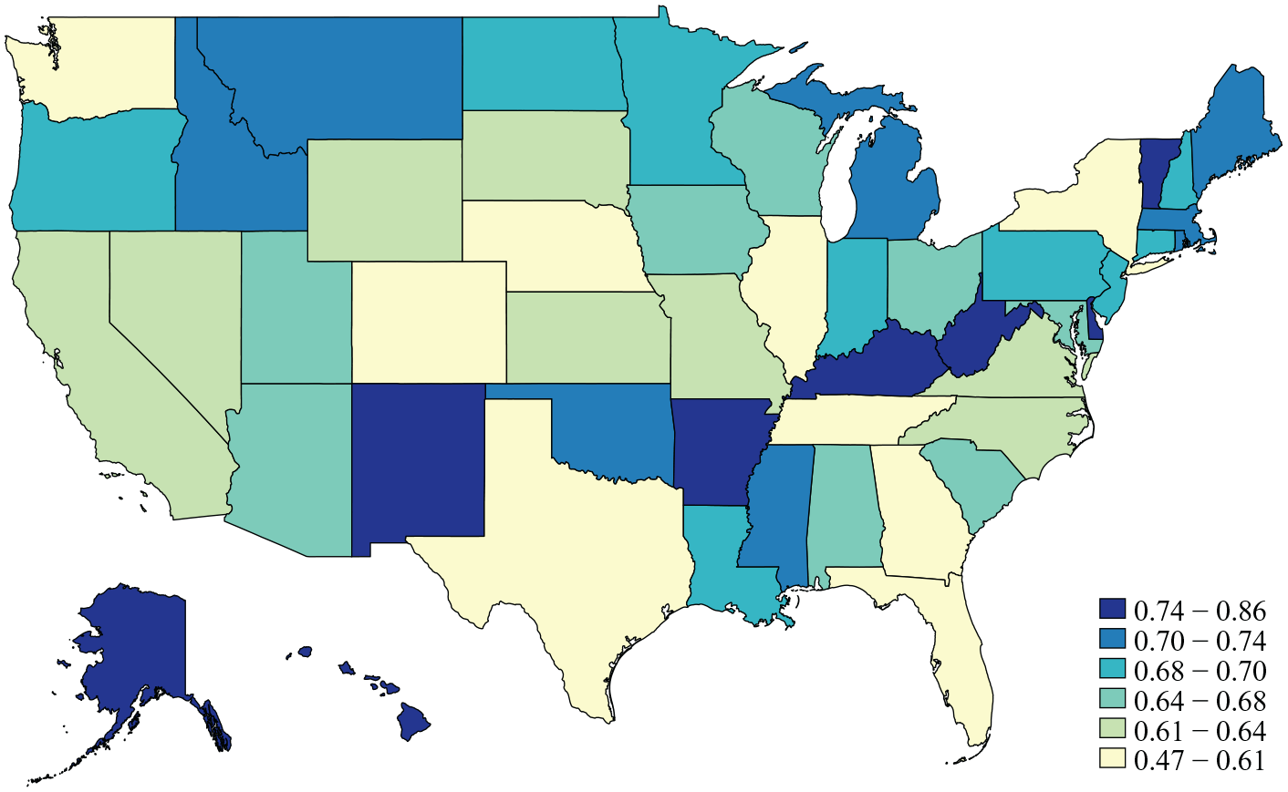
Expenditure Centralization of U.S. States (2017)

Unlike states, local governments are not fiscally sovereign; their fiscal authorities (e.g., use of revenue instruments like income or sales tax) and responsibilities (e.g., for financing police or roads) can be abridged or expanded, pursuant to state-specific procedures for doing so. In fact, states have the legal authority to create or destroy fiscal jurisdictions, for example, cities, towns, or school districts. The result is that even within states, there is often substantial variation in the relative role of counties, cities, towns, and districts in raising and spending public dollars and delivering public services. Here, too, centralization provides one useful descriptive metric of the local fiscal structure.

Figure 2 displays the fraction of total local government spending in each county performed by the county government, which is typically the local government at the highest level of spatial aggregation. Here again we see clear differences across states. For example, local governance in Virginia, North Carolina, and Tennessee—states that have historically empowered county governments—is relatively centralized, particularly compared to the southern New England states that eschew county government entirely and vest all local policymaking in cities and towns. There is also substantial variation within states, as county governments share responsibilities to different extents with more granular fiscal jurisdictions (cities, towns, special districts).

Figure 2.

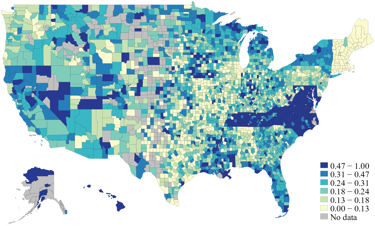
Expenditure Centralization of U.S. County Areas (2017)

Variation in expenditure centralization does not map on to contemporary political cleavages, that is, there is no discernable pattern across red (Republican) and blue (Democratic) states or localities. Nor is there a clear distinction between urban and rural locales or systematic variation as a function of local economic structure, such as the presence of manufacturing or the intensity of agriculture. What, then, explains this variation in the degree of expenditure centralization, both within and between states?

Fiscal Centralization: Origins and Persistence

Why are some fiscal structures more centralized than others? In a comparative analysis, Panizza (1999:120) concludes “that history is very important” in explaining cross-national variation in fiscal centralization. In evaluating accounts for why some U.S. states are more centralized than others, Stonecash (1988:82) similarly emphasizes “that state histories, traditions, and responses to unique events” have more explanatory power than economic or political characteristics: Hawaii’s relatively centralized fiscal structure can be traced back to its “heritage of a royal kingdom in which all power was held by the king,” whereas the “New England states are relatively decentralized because of a long tradition of local autonomy.” Cross-state differences in centralization today are the result of place-specific histories of fiscal governance, with the largest structural changes occurring in the aftermath of the Civil War and during the Great Depression (see Coen-Pirani and Wooley 2018).

To illustrate how path dependent histories drive the disparate fiscal centralization levels we observe today, consider the neighboring states of Arkansas and Tennessee. As Figure 1 demonstrates, Arkansas has a relatively centralized fiscal structure, with the state government performing the bulk of public spending. Tennessee, by contrast, has a decentralized system, with local jurisdictions, particularly county governments, playing a greater fiscal role. How did neighboring states come to have such disparate fiscal structures?

Founding stories reveal the fiscal governance structure of these two states differed from the very start. Tennessee’s history begins before the Revolutionary War, when settlers on the western edge of British colonial America formed what became known as the Washington District (later Washington County) and petitioned Virginia (unsuccessfully) and North Carolina (successfully) for annexation (Laska 1975, 1990). In a bid to reduce its revolutionary war debts, North Carolina would soon cede these lands back to the federal government, setting this collection of counties on its own path to statehood in 1796. Whereas Tennessee was founded and grew through the incorporation and annexation of counties, Arkansas’ origins are quite different: the land was acquired as part of the Louisiana purchase in 1803 (after stints under Spanish and later French administration) and was organized and administered as a territory until its admittance into the Union as a slave state in 1836, four decades after its neighbor to the east. Put simply, the fact that Tennessee has a relatively decentralized fiscal structure with fiscally important county governments, whereas neighboring Arkansas has a relatively centralized structure with a fiscally powerful state government, is traceable to policy decisions made more than two centuries ago.

The constitutional history of these neighboring states reveals how these initial differences became reified over time. Having seceded in 1861, both states drafted new constitutions after the Civil War as a requirement for re-admittance to the Union. Arkansas adopted a new constitution in 1868 and then again in 1874 (Goss 2011); Tennessee in 1870 (Laska 1990). Although drafted in the same historical moment, the documents differ in many important respects, including the amendment process, which was made considerably harder in Tennessee than in Arkansas. This, coupled with the extreme detail of the Arkansas constitution, led Arkansans to view the constitution as a place to enshrine law and turned the amendment process into a battlefield for fights over the allocation of fiscal powers and obligations across jurisdictions. In the nearly 150 years since ratification, 169 constitutional amendments have been proposed to the Arkansas Constitution, with 77 ultimately adopted (Goss 2011:15). Tennessee’s constitution, in contrast, would set a record for going the longest period unamended; by the time Tennessee adopted its first amendment in 1953 (Laska 1975), Arkansas had already adopted 42 amendments and rejected many others.

Strict limits on the property tax rates set by county and municipal governments were among the first amendments to the Arkansas state constitution. Whereas Arkansas was an early leader in restricting local property taxes, Tennessee would enter the twenty-first century as one of only a handful of states without any type of state limit on property taxation (see Paquin 2015). That Arkansas was an early mover in restricting local government use of the property tax whereas Tennessee enacted no such restrictions served to reinforce and entrench differences in their fiscal structure.

As this brief comparative historical analysis reveals, the different fiscal structures Arkansans and Tennesseans inhabit today are the cumulative result of contingent, place-specific histories unfolding over time. The particular fiscal structures of these two states, or of the other 48, should therefore not be readily ascribed to the preferences of today’s residents. This historical lens undermines a key assumption of the Tiebout (1956) model, dominant in the study of public finance, which holds that residence in a place should be taken as a resident’s “revealed preference” in favor of that place’s tax and spending policies. If not, the Tiebout model holds, residents would vote to change the system or “vote with their feet” by moving to another jurisdiction. Yet, as sociologists have long recognized, place is typically not chosen, but instead assigned by birth or the vicissitudes of human social life (Dahl and Sorenson 2010; Speare, Kobrin, and Kingkade 1982). People move for reasons of family or work or love, rarely with the explicit motivation of finding a more desirable fiscal structure (even among the wealthy, see Young 2017; Young et al. 2016). Residents today inhabit fiscal structures built by generations past, wherein citizens and policymakers engage in incremental battles over taxing and spending within the broad contours of the system they inherited.

The upshot of this path dependence is that while fiscal centralization is not fixed over time it is rather sticky. Figure 3 presents scatter plots comparing expenditure centralization in 1977 and 2017 for all U.S. states (left) and counties (right). We see a close correspondence between the two time periods at both levels of governance, with correlation coefficients of 0.83 for states and 0.93 for counties. The persistence of centralization is remarkable given the tremendous social and economic change of the past four decades, most notably the increasing inequality between households and between places (see Ganong and Shoag 2017; Manduca 2019). As Schumpeter ([1918] 1991:111) argued, the tax state is “shot through with elements of the past,” and its structure determines not only the scope and nature of politics, but also the nature of inequality across places.

Figure 3.

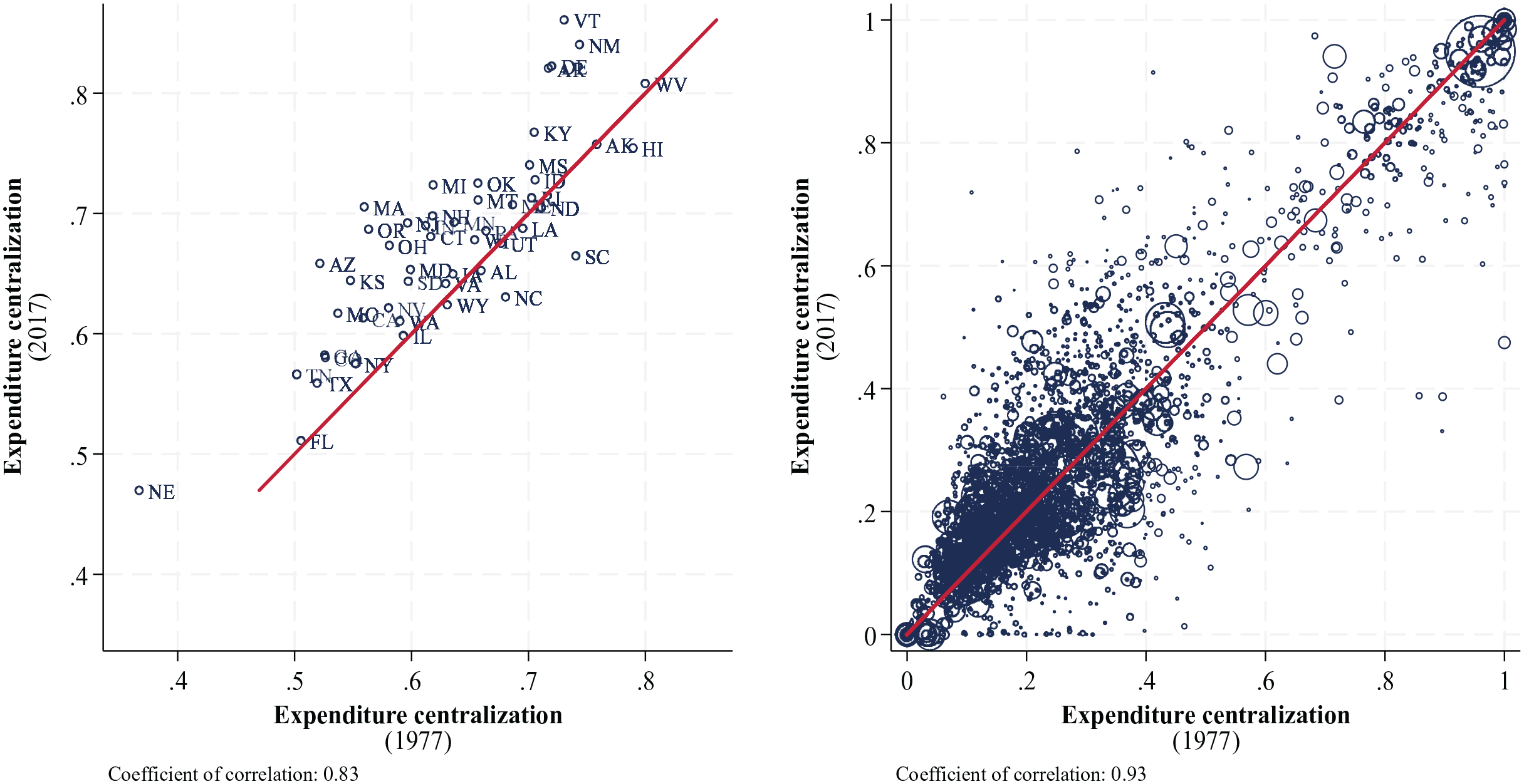
Expenditure Centralization of States (left) and Counties (right) in 1977 and 2017

Fiscal Centralization and Place Effects: Theory and Measures

Prior research in economics and political science has considered how fiscal centralization affects national economic growth rates and the degree of economic inequality between subnational regions. This comparative, cross-national work hypothesized that countries with more decentralized fiscal systems would tend to exhibit greater economic inequality between regions and, by extension, between households (Bosch and Espasa 2010; Dragu and Rodden 2011; Neyapti 2006; Oates 1968, 1999; Prud’homme 1995; Rodden 2010; Yeung 2009). Recent empirical work has challenged this expectation, finding decentralized systems actually facilitate regional economic convergence (Canaleta, Arzoz, and Garate 2004; Qian and Weingast 1997; Weingast 1995), thereby reducing inequality across households (Sepulveda and Martinez-Vazquez 2011; Sorens 2014). Yet Beramendi (2003, 2007, 2012) suggests the causal arrow may work in the other direction, arguing countries with more regional economic inequality were more likely to adopt decentralized systems in the first place (see also Kyriacou, Muinelo-Gallo, and Roca-Sagalés 2017). Overall, the cross-national scope of this literature makes it difficult to disentangle the effect of centralization from other aspects of policy and economic context, such as political institutions, welfare state generosity, economic growth, and political capacity.

In this study, we take a different approach. Instead of focusing on variation in fiscal centralization between countries, we examine variation across systems within a single country. This enables us to isolate the effect of centralization from myriad potential confounders inherent to analyses of nation-states. We also depart from research examining regional economic con(di)vergence to instead consider whether and to what extent centralization shapes the overall degree of spatial inequality or variation in the effect of place on life chances. We hypothesize that place-based differences will be lower in more centralized fiscal systems, that is, centralized systems will exhibit less spatial inequality in social outcomes.

Testing this proposition requires a measure of spatial inequality that does not conflate compositional features of a place with the effect of the place itself. When comparing any two places (e.g., states or cities or counties or school districts), analysts typically consider similarity and difference on a range of economic (e.g., poverty and unemployment rates, median household income) and demographic (e.g., age distribution, percentage Black residents) characteristics. These measures provide a useful basis for comparing the composition of places. But compositional differences are not necessarily the result of place-based or place-specific social processes. That is, we cannot take the fact that community A has more poor residents than community B as evidence that community A—its institutions (e.g., schools), labor markets, social policies, or built environment—impoverishes its residents more than community B. Compositional differences between places can result simply from patterns of migration and settlement, both historic and contemporary, as well as through the varied effects of large-scale macroeconomic change, for example, the decline of manufacturing and the rise of the information economy, that makes some places poor and others rich.

Uncovering the effect of place requires us to compare how life outcomes differ among similar individuals exposed to different contexts. One way is through experiments, such as the well-known Moving to Opportunity Study (Sampson 2008), wherein households were randomly chosen to receive housing vouchers, some with the stipulation they move to lower-poverty neighborhoods. Evidence indicates the children exposed to better contexts went on to achieve greater educational attainment and higher earnings than their otherwise similar peers who remained in high-poverty communities (Chetty et al. 2016). “Natural” experiments, such as displacement following a natural disaster (e.g., Schnake-Mahl et al. 2020), can also be leveraged to examine the causal effect of place on outcomes over the life course, as can “quasi-experimental” methods—including propensity score matching, instrumental variables, and regression discontinuity designs—that are frequently used to overcome selection and composition biases to recover the effect of place.

Our approach is to measure the extent to which individuals’ outcomes differ across census tracts within a state or county area. We do so with data from Opportunity Insights (OI), who use population-level, administrative tax data on household income to estimate the predicted adult intergenerational economic mobility outcomes of children from the same birth cohort and raised by parents at the same percentile of household income. The OI mobility estimates are, to our knowledge, the only population-based estimates of a social outcome available at the census-tract level that conditions on both age and income (and can be further conditioned on race and sex, as we examine in our robustness checks)—thus offering a more effective way to disentangle the effect of place from the demographic composition of place than is typically feasible with observational data.¹ Measuring cross-census tract variation in the predicted mobility outcomes of comparable children captures the overall degree of spatial inequality within a state or within a county in the effect of place on life chances.

Our motivating hypothesis is that in more centralized fiscal systems, there will be less variation in the effect of place on life chances and therefore less spatial inequality in economic mobility. That is, we expect to find economic mobility outcomes to be more similar across places in centralized systems and to be more different across places in decentralized systems. Why? We theorize that fiscal centralization reduces spatial inequality by leveling up the worst-performing census tracts in a county area. The reasoning is straightforward: in decentralized county areas, the boundaries of local fiscal jurisdictions reinforce place-based differences in social need and taxable wealth; some towns will have high poverty and low fiscal capacity, whereas others will have low poverty and high fiscal capacity. By contrast, in centralized county areas, the bulk of government spending and services are performed by the county government, permitting resources to be extracted from wealthy areas and targeted to areas with high social need. This, coupled with research showing the effect of government spending on social outcomes is greater for low-income people and places (e.g., Biasi 2021; Rauscher and Shen 2022), suggests centralization will reduce spatial inequality in social outcomes specifically by leveling up the lowest-performing areas. If our hypothesis is correct, centralization should mechanically yield a higher mean or overall mobility level in a county area.

To further build our intuition, let us consider the three ways fiscal centralization is operationalized in the literature and how each suggests distinct pathways through which greater centralization should yield less spatial inequality in social outcomes overall. All three paths should dampen spatial inequality by enhancing outcomes in the worst-performing places.

Total Expenditure Centralization

This is measured as the fraction of total government spending performed by the central or higher-level government. As noted earlier, this is the most common measure of fiscal centralization; it can be constructed at the national level as well as for states and counties by simply calculating the total fraction of government spending within a system performed by the higher-level government. There are several reasons why we should expect variation across places to be lower in systems where spending is more centralized. For one, if the central government does relatively more of the total government spending, that means fewer dollars are spent at the lower level; mechanically, this should result in lower absolute inequality in spending levels across local jurisdictions. At the same time, locating spending at the higher level of government typically subjects those dollars to greater democratic scrutiny, increasing the likelihood dollars are allocated to institutions (e.g., schools) and households pursuant to finance formulas or other scrutable bureaucratic procedures; this should typically target more resources to areas with higher social need. Moreover, greater economies of scale may enable more efficient spending of public dollars; and those dollars may have greater efficacy given that higher-level governments tend to have more professional bureaucracies with greater substantive expertise. Taken together, we should expect to find less spatial inequality in fiscal systems where total government spending is more centralized.

Own-Source Revenue Centralization

This is measured as the fraction of total own-source revenues in an area collected by the higher-level government. “Own-source” revenue refers to dollars collected by a government pursuant to taxes or fees it levies directly. This is distinct from “intergovernmental (IG) revenue,” which are dollars provided by another government. For example, the state of California provides substantial IG revenue transfers to county governments to administer Medicaid services, and many state governments provide IG revenue transfers to local governments to support K–12 education. Whereas IG revenue comes with strings and oversight, governments typically have more discretion over how to spend own-source revenue. Indeed, in political science and public administration research, own-source revenue levels are often taken as a measure of a government’s “fiscal autonomy,” that is, the extent to which a government has control over its fiscal policymaking (see, e.g., Dougherty, Harding, and Reschovsky 2019). In fiscal systems where the policymaking power is centralized at the higher-level government, we should expect to find relatively less place-based variation in the quality and intensity of the local public sector, and by extension, less spatial inequality in social outcomes. In decentralized systems, a town or district may not have sufficient taxable wealth within its borders to meet social needs with own-source revenues; by contrast, in centralized systems where revenue can be drawn from a larger geographic area, there is greater potential to raise public funds sufficient to meet social needs.

Public Employment Centralization

This is measured as the fraction of total public workers in an area employed by the higher-level government. For example, at the national level this would be federal government workers as a fraction of all government employees in the United States; at the state level this is measured as the fraction of state and local public workers employed by the state government; and at the local level this is the fraction of all local government (e.g., county, city, town, district) workers employed by the county government. Here the intuition is that it is not just taxing and spending that matters, but the level of government tasked with the direct provision of government services. If a relatively greater share of the total public workforce is employed by the higher-level government, we should expect the quality of public services—and, by extension, social outcomes—to be more similar across places. By extension, poorer areas will receive higher-quality public services than they would otherwise be able to afford in a decentralized structure.

How correlated are these measures of fiscal centralization? Figure 4 displays the correlation matrix for centralization of government expenditure, own-source revenue, and public employment centralization, as well as the per capita amount of government expenditures, own-source revenues, and public employment, separately for states and for counties. First, note that expenditure centralization and own-source revenue centralization are highly correlated across both states and counties; where the higher-level government collects more of the revenue, it is also likely to spend relatively more of the total public dollars. Employee centralization and expenditure centralization are highly correlated at the county level, but notably not at the state level; whereas counties that spend relatively more of total local government dollars also employ relatively more of the local government personnel, state governments that contribute a relatively greater share of total state and local government spending do not necessarily employ a relatively greater share of total state and local government workers. These patterns underscore how each measure of fiscal centralization provides related but distinct insights into how fiscal policymaking is located hierarchically.

Figure 4.

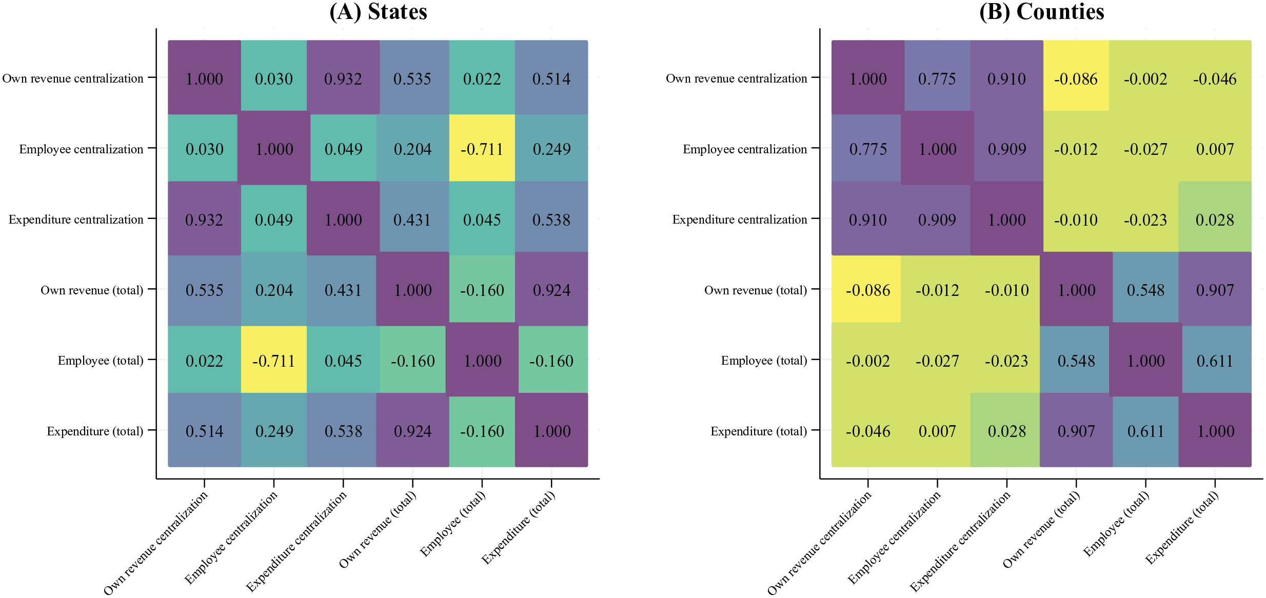
Correlation Matrix of Fiscal Centralization and Fiscal Levels across U.S. States (left) and Counties (Right)

Note, too, the correlation matrix reveals measures of fiscal centralization are not correlated with measures of fiscal levels, that is, total amount of per capita government spending, own-source revenue, or public employment. We find no evidence that local public sectors in more centralized fiscal systems are any more or less intensive or generous than public sectors in more decentralized systems. That the total amount of government spending (and revenue and employment) in a fiscal system is independent of its centralization provides further motivation for empirically investigating whether and how the latter independently shapes spatial inequality in social outcomes. Yet despite their empirical and conceptual independence, we do expect there to be a relationship between fiscal centralization and fiscal levels (e.g., total spending) in models predicting spatial variation in social outcomes. Specifically, we expect the (spatial) equalizing effect of fiscal centralization to be greater in areas with more total government activity. Put simply, the potential for fiscal centralization to reduce variation across places is greater in areas where there is more overall fiscal action (spending, revenues, employment) to be centralized.

Data and Analytic Approach

Outcome Variable: Spatial Inequality in Economic Mobility

We measure variation in the effect of place on life outcomes using data from Opportunity Insights (Chetty et al. 2014), who provide place-based estimates of the intergenerational economic mobility outcomes of children born between 1978 and 1983. Our primary measure of intergenerational economic mobility is the predicted mean income percentile rank achieved in adulthood (approximately age 34) by children born to families at the 25th percentile of national household income. To capture the overall degree of spatial inequality mobility outcomes, we estimate the coefficient of variation (CoV) across all census tracts within a state and, separately, within a county area, weighting each census tract by the number of children in the mobility cohort. The coefficient of variation is the standard deviation divided by the mean; it provides a scale invariant measure of the extent to which outcomes differ across census tracts. As we restrict our mobility measure to children from the same birth cohort raised in households at the same income and in the same state or county, a larger CoV indicates greater variation or inequality in the effect of place on life outcomes. Our primary measure considers mobility outcomes for the full population cohort; we also construct a measure of spatial inequality in the mobility outcomes of low-income white males as a robustness check to rule out confounding by spatial variation in structural racism (and sexism) and racial residential segregation.

Figure S1 in the online supplement shows the distribution of the county-area CoV in mobility outcomes for the full population cohort; and Figure S2 maps mobility variation across states and counties. Descriptive statistics are in Table S1 in the online supplement.

Independent Variable: Fiscal Centralization Index

We measure fiscal centralization using data from the U.S. Census of Governments, a survey conducted every five years (in years ending in 2 and 7) that details the revenues and expenditures of every fiscal jurisdiction in the United States. In our analyses, we use data from 1992, when the focal cohort was in early adolescence (age 9 to 14), a critical period when contextual exposures can have lasting effects on life course development. This year also best approximates the year parental income is measured for the mobility estimates. It therefore also best captures when children are observed to reside in the focal census tract. By 1997, the next year fiscal data are available, many children will have left their parents’ home to pursue higher education or start their own household.

We operationalize fiscal centralization by constructing an index that combines the three measures of centralization detailed earlier: expenditure centralization, own-source revenue centralization, and public employment centralization. At the state level, estimating these component measures is relatively straightforward, simply the fraction of the total state and local spending, own-source revenue, and employment performed by the state government.

Measuring centralization at the local level is more complex due to cross-state differences in the structure of local fiscal governance. To craft a measure that is broadly comparable across states, we first aggregate government spending, own-source revenue, and public employment within a county area, summing across all local government types (e.g., county, municipal/town, district). We then construct centralization measures as the fraction of total spending, own revenue, and employment within a county area performed by the county government. We do this for several reasons. First, counties are typically the local government type that sits at the highest level of spatial aggregation. Second, in most states, local fiscal jurisdictions such as municipalities and school districts respect county borders, which makes it straightforward to estimate the total amount of government spending within a county area. Third, there is wide variation both across and within states in the fiscal role of county governments; we harness this variation in our analysis.

For each state and for each county, the above yields three measures of centralization (expenditure, own-source revenue, public employment), each scaled from 0 (fully decentralized) to 1 (fully centralized). We then standardize and combine these measures into a single index; this process yields a Cronbach’s Alpha of 0.85 at the state level and 0.96 at the county level, indicating a high degree of internal consistency, as expected given the correlation between these measures.

Analytic Approach

We begin by examining the relationship between fiscal centralization and spatial inequality in economic mobility at the state level. We first estimate the bivariate association and then adjust for total state and local expenditures (per capita), own-source revenues (per capita), and public employees (per capita) to rule out these obvious potential confounders. Given the relatively small number of states, and the marked policy and institutional differences between them, these results should be viewed as suggestive but not conclusive given our research design.

We then turn to our primary analysis examining this relationship at the local level. We estimate four models:

Y_{c s} = α_{1} F i s c C e n_{c} + μ_{s} + e_{c s}

(1)

Y_{c s} = α_{1} F i s c C e n_{c} + μ_{s} + β_{1} X_{c} + e_{c s}

(2)

Y_{c s} = α_{1} F i s c C e n_{c} + μ_{s} + β_{1} X_{c} + β_{2} Z_{c} + e_{c s}

(3)

Y_{c s} = α_{1} F i s c C e n_{c} + μ_{s} + β_{1} X_{c} + β_{2} Z_{c} + β_{3} S_{c} + e_{c s}

(4)

We first estimate the relationship between county-area fiscal centralization () and CoV in mobility outcomes () net of state fixed effects () (Equation 1). Restricting our comparison to counties within the same state ensures our findings are not being driven by other features of state fiscal systems or social and economic policy. Equation 2 then adjusts for, a vector with terms capturing the amount of per capita total expenditures, own-source revenues, and public employment summed across all jurisdictions in the county area.

Equation 3 includes a vector of social, demographic, and spatial covariates, including the number of census tracts in the county with mobility data (logged), the county population (logged), a five-category rurality index, household poverty rate, median household income, share of manufacturing jobs (Eckert et al 2021; Seltzer 2024), and the cross-tract variation (CoV) in household poverty, median income, and share of single-parent households, all estimated from the 1990 decennial census. This vector also includes the total county land area in square miles (logged), as well as the Gini segregation index (Escarce, Lurie, and Jewell 2011) to capture racial residential segregation in the county in 1990, and cross-tract variation in job density in 2013 to capture spatial variation in local labor markets. Finally, Equation 4 includes S_c to adjust for other measures of local fiscal structure in the county, including the number of general-purpose governments (logged), number of special districts (logged), and school districts (logged).

In all models we cluster standard errors at the state level to account for fiscal interdependence of local governments in the same state. After listwise deletion, our final analytic dataset comprises 2,830 counties; descriptive statistics for all measures are presented in Table S1 in the online supplement.

Results

We begin by descriptively investigating the association between fiscal centralization and spatial inequality in mobility outcomes at the state level. Figure 5 plots this relationship. Consistent with expectations, we find that in states with more centralized fiscal systems, there is less cross-census tract variation in the economic mobility outcomes of low-income children. Note the relative positions of Tennessee (TN) and Arkansas (AR), neighboring states with remarkably different fiscal structures resulting from contingent historical trajectories detailed earlier; there is less spatial inequality in the mobility outcomes of low-income children in fiscally centralized Arkansas compared to decentralized Tennessee.

Figure 5.

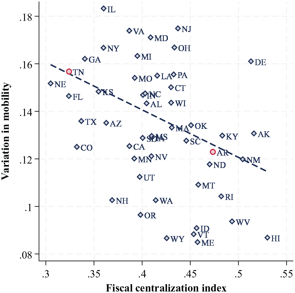
Fiscal Centralization and Within-State Mobility Variation (CoV)

Corresponding to the fitted line in Figure 5, Model 1 in Table 1 presents the estimated coefficient on our state fiscal centralization index in a bivariate model predicting the cross-census-tract variation or inequality in the mobility outcomes of low-income children in the state. Results from Model 2 show this association holds after adjusting for the total amount of (state and local) government spending in the state; results from Model 3 find the association remains negative after also adjusting for the per capital total own-source revenue; and Model 4 shows the relationship is robust to adjusting for the level of per capita total public employment in the state. Note the estimated coefficient on our fiscal centralization index is unaffected by including measures of total per capita spending, revenues, and public employment and, notably, these measures are not independently associated with the overall amount of spatial inequality within states.

Table 1.

Fiscal Centralization and Spatial Inequality in Mobility, U.S. States

	Model 1	Model 2	Model 3	Model 4
Fiscal centralization index	–.408** (.132)	–.447** (.161)	–.433** (.161)	–.400* (.170)
Total expenditure per capita		.068(.161)	–.545(.536)	–.501(.544)
Total own-source revenue per capita			.626(.522)	.592(.528)
Full-time equivalent employees per capita				.093(.149)
N	50	50	50	50

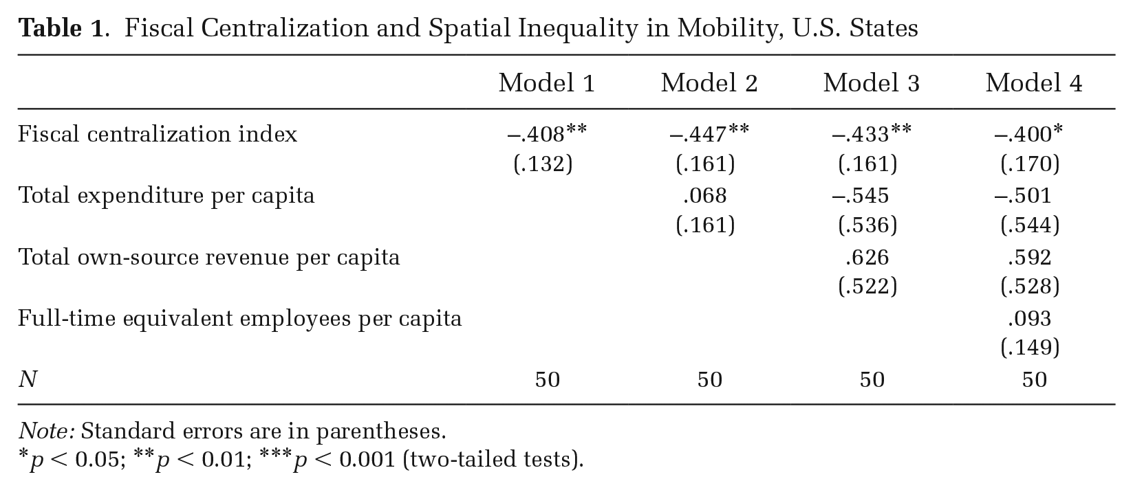
Note: Standard errors are in parentheses.

p < 0.05; **p < 0.01; ***p < 0.001 (two-tailed tests).

Of course, states vary on a range of dimensions—from their economic and social policies to their industrial mix and political institutions—that may be correlated with fiscal centralization and shape spatial variation in the effect of place; too many dimensions to adequately adjust for in a model with only 50 observations. We therefore turn to our primary analysis, which investigates within-state variation in spatial inequality across counties.

Figure 6 plots this relationship at the county level net of state fixed effects; each dot corresponds to a bin of 50 county observations. The figure reveals a clear inverse relationship between county-area fiscal centralization and the within-county coefficient of variation in mobility outcomes. In county areas where relatively more of the total government activity is performed by the county government, there is relatively less spatial inequality in the predicted mobility outcomes of low-income children.²

Figure 6.

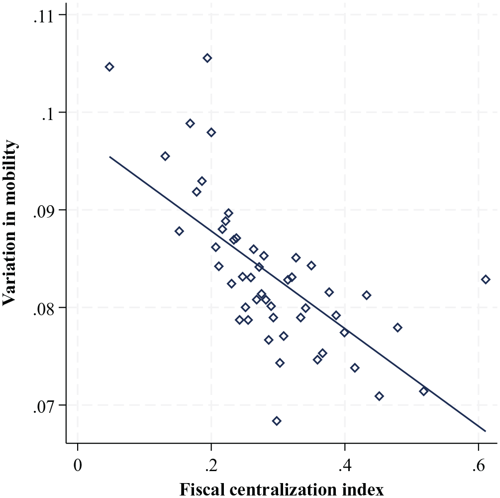
Fiscal Centralization and Within-County Mobility Variation (CoV); Linear Association Net of State Fixed Effects

Table 2 summarizes results from our multivariable analyses, displaying the estimated coefficient on county centralization across each of our four model specifications (for full regression results, see Table S2 in the online supplement). Model 1 presents estimates from the bivariate model net of state fixed effects (Equation 1), corresponding to the fitted line in Figure 6. The estimated coefficient indicates that a one standard deviation increase in fiscal centralization is associated with about 25 percent of a standard deviation less spatial inequality in mobility across census tracts in a county area.

Table 2.

Fiscal Centralization and Spatial Inequality in Mobility, U.S. Counties

	Model 1	Model 2	Model 3	Model 4
Fiscal centralization index	–.255*** (.054)	–.230*** (.055)	–.095** (.031)	–.100** (.030)
Full-time equivalent employees per capita		–.126*** (.034)	.049(.027)	.049(.027)
Total expenditure per capita		.189(.125)	.030(.076)	.029(.081)
Total own-source revenue per capita		.148(.112)	.013(.062)	.014(.065)
Fiscal structure covariates				Yes
County characteristics			Yes	Yes
State fixed effects	Yes	Yes	Yes	Yes
N	2,830	2,830	2,830	2,830

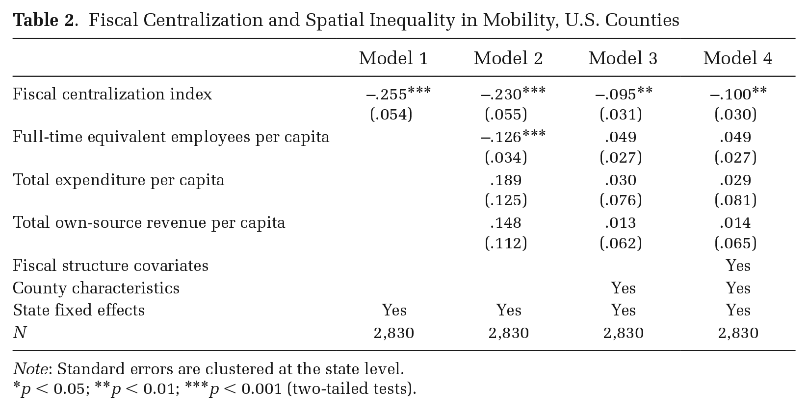
Note: Standard errors are clustered at the state level.

p < 0.05; **p < 0.01; ***p < 0.001 (two-tailed tests).

Results from Model 2 (Equation 2) demonstrate this relationship is robust to adjusting for per capita government expenditures, own-source revenues, and employment within the county area, demonstrating the effect is not driven by local government intensity. Model 3 (Equation 3) shows the association holds after adjusting for a host of county-area social, economic, and demographic characteristics, including racial segregation, county population, median household income, and the household poverty rate and spatial variation in household income and poverty. Finally, Model 4 (Equation 4) adjusts for other aspects of local fiscal structure, including the total number of general-purpose governments, school districts, and special districts.

In our fully adjusted model (Model 4), the estimated coefficient indicates a one standard deviation increase in our fiscal centralization index is associated with 10 percent of a standard deviation less spatial inequality in the economic mobility outcomes of low-income children. To benchmark this effect size, note that estimates from the same model indicate a one SD decrease in cross-tract variation in household poverty is associated with 13 percent of an SD less spatial inequality in economic mobility. While the spatial patterning of disadvantage is a key determinant of spatial inequality in mobility outcomes, our findings reveal that so, too, is the fiscal system in which those places are embedded.

In the analysis above, we include total per capita government spending in the county area as a covariate in the model; this permits us to estimate the effect of fiscal centralization net of spending. Yet, as noted, we should expect the equalizing effect of fiscal centralization to be greater in areas with relatively more spending, that is, where there is more fiscal action to be centralized. To examine this, we divided counties into five subsamples by quintile of total government spending per capita. We then re-estimated our model (Equation 4) on each subsample and plotted the coefficient on our fiscal centralization index. Consistent with expectations, Figure 7 illustrates that the estimated effect of fiscal centralization on spatial inequality in mobility outcomes is stronger in county areas with relatively more total government spending per capita.

Figure 7.

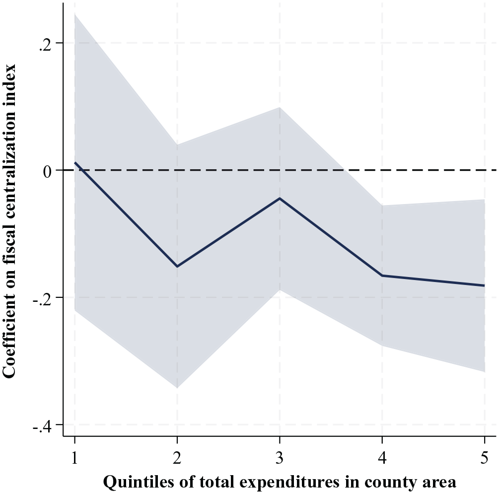
Estimated Coefficient on Fiscal Centralization Index for Each Quintile of Total County-Area Per Capita Government Spending

How Does Centralization Reduce Spatial Inequality in Mobility?

Our analysis demonstrates that more centralized fiscal systems exhibit less within-county variation across census tracts in the upward mobility outcomes of low-income children; and this equalizing effect of centralization is amplified at higher levels of total per capita local government spending. As noted earlier, less spatial inequality within a county can be achieved through a leveling up of low-performing census tracts—a desirable outcome—or through a leveling down of high-performing census tracts—an undesirable outcome—or some combination of both. As government interventions typically have the most profound effect on the outcomes of low-income households and communities, and our theory posits that more centralized structures are better equipped to allocate resources to areas in need, we hypothesize that fiscal centralization reduces spatial inequality by leveling up the lowest-performing census tracts in a county area.

To investigate this, we ordered census tracts in each county from lowest to highest based on the level of upward mobility achieved by low-income children. We then re-estimated our primary model specification using fiscal centralization to predict the upward mobility level achieved in the 10th percentile census tract in each county, and subsequently for the 20th percentile and so on. Figure 8 presents the estimated coefficient on fiscal centralization on the mobility outcomes in each census-tract decile. The results indicate that fiscal centralization has a substantial, positive effect on the mobility outcomes of the worst-performing (10th percentile) census tracts in each county, with the effect diminishing monotonically across higher deciles. Notably, the estimated coefficient remains positive at even the 90th percentile census tract in each county, although it is not statistically different from zero. This provides strong evidence that fiscal centralization reduces spatial inequality by leveling up the worst-performing census tracts in a county, without any indication of leveling down the highest-performing tracts. This trend in coefficients is not an artifact of the model. Bivariate (net of state fixed effects) scatterplots in Figure S3 in the online supplement reveal that mobility levels achieved in the 10th percentile census tract are relatively higher in more centralized counties, with no similar pattern observed at the 90th percentile census tracts.

Figure 8.

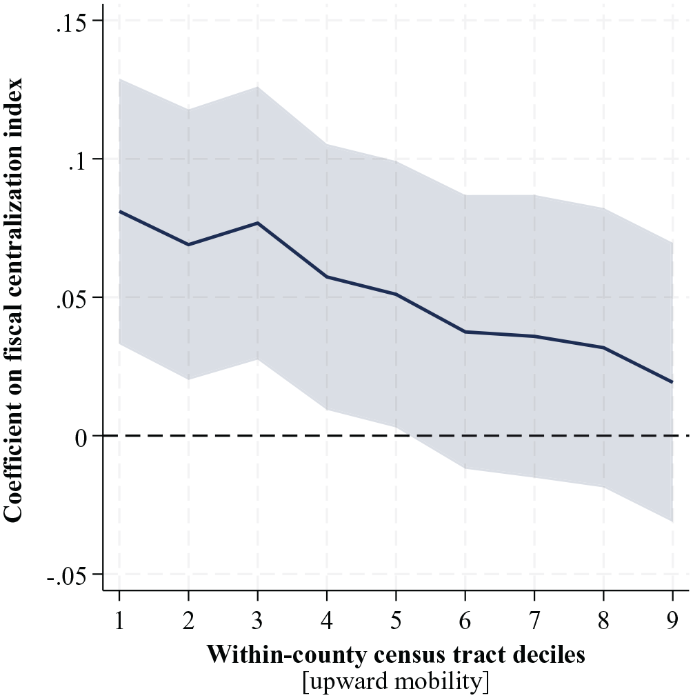
Estimated Coefficient on Fiscal Centralization Index for Each (Within-County) Census Tract Decile of Upward Mobility Outcomes

Ultimately, as fiscal centralization reduces spatial inequality by leveling up the worst-performing census tracts in a county—with no effect on the best-performing census tracts—we should expect centralization to be positively correlated with the mean or overall mobility level in the county. Table S3 in the online supplement shows this is indeed the case. Specifically, we find a one standard deviation increase in our fiscal centralization index is associated with about 7 percent of a standard deviation improvement in the mobility outcomes of low-income children in a county area. As a benchmark, in their fully adjusted model, Chetty and colleagues (2014; see their online Appendix Table VIII) find a one standard deviation increase in local government per capita expenditures is associated with 10 percent of a standard deviation improvement in the mobility outcomes of low-income children. This further underscores how the location of government spending can be almost as consequential as the level or amount of government spending in shaping social outcomes in a given area.

Robustness Checks and Sensitivity Analyses

Our findings provide direct evidence of an association between fiscal centralization and the degree of spatial inequality in life outcomes for children from the same birth cohort, level of household income, and state or county of residence. This association obtains net of the overall level of government spending, the total number of fiscal units, and the economic characteristics of the county, including the spatial patterning of income and poverty. We perform several robustness checks to address potential counterarguments and evaluate the consistency of our findings across reasonable alternative model specifications.

First, we consider the possibility that our findings are driven by the centralization of a specific category of local government spending; for example, our measure may simply be proxying for the relative role of county governments in K–12 education finance, an important determinant of mobility outcomes (Biasi 2023; Logan, Minca, and Adar 2012; Owens 2018).³ We examined this possibility by constructing measures of county-area fiscal expenditure centralization for eight different spending categories: K–12 education, higher education, public safety, housing and environment, administration, transportation, health and welfare, and interest on debt. We then re-estimated our primary specification (Equation 4) sequentially substituting these category-specific measures of fiscal expenditure centralization for our index. Figure S4 in the online supplement presents the estimated coefficient from each model. The coefficient on each type of expenditure centralization is negative and of similar magnitude. This provides assurance our findings are not driven by any specific local government service or function, but instead are due to the overall centralization of the fiscal structure.⁴

Second, we consider the possibility that our results may be sensitive to how we handle special district expenditures, revenues, and employees. Of all local government types, special districts are particularly heterogeneous in scale, from covering just part of a town to several county areas, and function, from financing of libraries, hospitals, airports, sewer, transit, water, conservation, fire protection, to even public cemeteries (Berry 2009). And while many special districts have tax and spending powers that mirror those of general-purpose governments, some generate substantial revenue through the sale of services. For example, many transit agencies operate as a special district, such as the Bay Area Rapid Transit (BART) system, with revenues largely dependent on transit user fees. In our centralization measure above, we treat special districts as we do local general-purpose governments, allocating expenditure, revenue, and employee levels to the county where the special district is headquartered. Although special districts account for only about one-tenth of local government spending, given vast differences in both function and geographic coverage, we test whether our results are robust to excluding these unique and disparate local fiscal units. To do so, we re-constructed our centralization measure excluding special district expenditures, revenues, and employees, that is, restricting our analysis to local general-purpose government and school districts. Our results using this alternative measure, presented in Table S7 in the online supplement, are nearly identical to those presented above.

Third, we considered that the fiscal structure of local governments and variation in mobility outcomes may be spatially correlated. Given the fiscal interdependence of counties in the same state, all models above include state fixed effects and cluster standard errors at the state level. Yet fiscal structures of neighboring localities may be correlated across state lines. We used the 2016 county shape files from the U.S. Census to construct a spatial weighting matrix using distance to county centroids. We used this weighting matrix to calculate Moran’s I and were not able to reject the null that there is zero spatial autocorrelation present (p = 0.23). This provides additional assurance that our findings are not driven by spatial interdependence. We also considered the possibility that, in some instances, counties might not be the appropriate spatial unit; for example, in states where jurisdictional boundaries of general-purpose local governments cross county lines. Aggregating data to the county area may introduce statistical bias that undermines inference (see Buzzelli 2019). To consider this possibility, we re-estimated our model on the subsample of states where local jurisdictional boundaries strictly observe county lines. The coefficient on our fiscal centralization index remains negative and the point estimate is slightly larger, consistent with county-area fiscal centralization being more precisely measured in this subsample of states (see Table S8 in the online supplement).

The online supplement also includes exhibits demonstrating results are robust to winsorizing the top 5 percent and bottom 5 percent values for our fiscal centralization index and our outcome measure (Table S9); sequentially excluding each state from the sample (Figure S4); weighting counties by number of children in the mobility sample (Table S10); and operationalizing spatial inequality in mobility outcomes using a “regional Gini index” instead of CoV (Table S11) (see Lee and Rogers 2019). We also find no relationship between county fiscal centralization and rates of in- or out-migration in the preceding decade (Table S12)

One potential confounder in our analysis is racial residential segregation. Historical and contemporary forces driving racial segregation concentrate Black Americans into not only specific neighborhoods but specific fiscal jurisdictions. Structural racism yields systematically different economic mobility outcomes for Black, Indigenous, and other minority groups relative to white children. So, too, will sexism and gender norms drive different mobility trajectories for girls versus boys. These social forces affect mobility processes directly and indirectly, for example, by moderating the effect of government spending so that the same public dollar has different effects for Black versus white children or for men versus women. To isolate the effect of place on the life outcomes of otherwise similar individuals, we therefore re-estimate our main models for white males only. Table S13 in the online supplement confirms our measure of variation in place effects is not confounded by residential segregation or the intensity of structural racism and sexism.

Finally, we disaggregate our centralization measure to examine the three components of our index—expenditure, own-source revenue, and employment centralization. To explore the relative importance of each in predicting spatial variation in economic mobility outcomes, Table S14 in the online supplement presents results from a dominance analysis that compares the fraction of unique shared variance explained by each measure of centralization. The dominance analysis treats the predictive model as a data-generating process with the fit statistic as the dependent variable. It allows us to decompose the overall model fit into each measure’s contribution. Findings reveal that own-source revenue centralization explains relatively more (51 percent) of the total shared variance followed by expenditure centralization (37 percent) and employee centralization (12 percent); in other words, own-source revenue centralization and total expenditure centralization dominates public employee centralization in accounting for differences across counties in the amount of spatial inequality in mobility outcomes. This suggests that beyond just spending, centralizing fiscal power and policymaking is key to reducing spatial inequality in life chances.

Discussion and Conclusions

Social scientists routinely document how disparities in subnational government spending drive spatial inequality in social outcomes, including economic mobility. In this study, we show it is not just the amount of government spending but the centralization of fiscal action in the hierarchy of governance that shapes the spatial patterning of life chances. Estimates from our fully specified model indicate that a one standard deviation increase in our county-area fiscal centralization index is associated with 10 percent of a standard deviation less spatial inequality in the mobility outcomes of low-income children. This association is estimated net of state fixed effects and a host of economic and demographic covariates, including total per capita government spending, revenue, and employment, as well as the number and type of local fiscal units, the spatial patterning of household income and poverty, and level of racial residential segregation. For context, the magnitude of this association is three-quarters as large as the estimated effect of spatial variation in poverty, a key correlate of place-based mobility outcomes in prior research. To ensure our findings are not confounded by spatial patterning of structural racism or sexism, we replicated our findings using a measure of spatial inequality restricted to white males only. We further demonstrate these associations are not confounded by the structure of K–12 education finance and are robust to a host of sensitivity analyses.

How does fiscal centralization reduce spatial inequality in social outcomes? We find it does so by leveling up the worst-performing census tracts in a county area, with no discernable effect on the best-performing tracts. Just as fiscal redistribution can improve outcomes in poor places by transferring resources to needy fiscal jurisdictions, fiscal centralization can improve outcomes in poor areas by pooling resources within a fiscal jurisdiction. This correspondence motivates a powerful site of policy intervention: if redistribution to poorer jurisdictions is not politically or administratively feasible, an alternative is to situate relatively more government action at the higher-level government, rendering lower-level jurisdictions—and the heterogeneity in their fiscal capacity—less determinative of life chances.

Conceptually, our work advances the study of subnational fiscal systems as an important, if often invisible, determinant of inequality across places. As we show, the centralization of fiscal systems varies markedly across U.S. states and counties. Moreover, these differences do not reflect variation in the current political, economic, or demographic profile of places, but are instead the cumulative result of history—contingent, place-specific negotiations over the relative fiscal role of overlapping jurisdictions, often codified in law or cemented in practice half a century ago or more. This historical path dependence is illustrated in tracing the fiscal evolution of Arkansas and Tennessee, neighboring states with vastly different fiscal systems. Beyond mere historical curiosities, our analysis demonstrates how these differences in the design of local fiscal systems affect spatial inequality today: the economic mobility outcomes of low-income children are more similar across census tracts in fiscally centralized Arkansas and more dissimilar across census tracts in fiscally decentralized Tennessee.

Future work is needed to further detail the mechanisms through which centralization leads to more equal outcomes across places. To facilitate this work, we will make public measures of fiscal centralization at the state and local level from 1977 to 2017. Empirical research should be augmented by fiscal histories to reveal the contingent origin of local fiscal structures and detail the rules, norms, procedures, and processes that drive inequalities across places today. Such a historical orientation is essential, if only to prevent the uncritical (and unconscious) assumption that differences in fiscal structure arise from and represent differences in the fiscal policy preferences of current residents. As Rudolf Goldscheid ([1925] 1958:206), a first-generation fiscal sociologist, noted long ago, “history, sociology and statistics of finance are the three pillars which alone can support a theory of public finance which is not totally divorced from reality.”

Deep analysis of fiscal systems can and should form the basis for a fiscal sociology of place that eschews the abstract models and process ideal-types that dominate traditional approaches to the study of public finance in favor of historically- and empirically-grounded interrogations of how tax and spending systems contribute to the production of place-based inequalities. Constructs and measures of state and local governance used in political science and public administration research—including not just centralization and redistribution but also government fragmentation, nesting, and local fiscal autonomy—can and should be deployed by sociologists to better reveal the structural drivers of fiscal inequities between places. This framework also provides a new lens for analyzing trends through time, for example, through investigating how fiscal structures interact with an evolving economy and social demography to mitigate or exacerbate emergent inequalities between places. This framework also helps us reconcile why some communities rely so intensely on fines, fees, and other regressive revenue instruments to finance the public sector and identify potential avenues for reform (Harris 2016; Harris, Patillo, and Sykes 2022; Pacewicz and Robinson 2021).

The benefit of naming fiscal structures as a macrosociological object is that it becomes something that can be analyzed, evaluated, organized around, and acted upon. This can facilitate a new type of problem-solving sociology (Prasad 2018, 2021). As Goldscheid ([1925] 1958:212) notes, “Every social problem and indeed every economic problem is in the last resort a financial problem.” Correlating social problems with fiscal disparities, however, is only the first step. The social analyst must then seek to understand how local economic and demographic trends interact with the local fiscal structure to generate fiscal inequalities or inadequacies across places. It is not inevitable that poor places have impoverished public sectors; it results from a fiscal structure that can be changed. Fiscal redistribution and centralization are two ways to improve fiscal equity, but they are not the only policy recourse. A fiscal sociology of place has the potential to motivate novel solutions to pressing social problems. The most effective policy solutions will target the fiscal structure itself. This includes changing the spatial boundaries that demarcate jurisdictions, altering their nested configuration and the allocation of fiscal obligations and powers between them.

A fiscal sociology of place requires an honest confrontation and reckoning with the past. Many constraints on state and local fiscal policymaking in the United States—from uniformity clauses (Einhorn 2008) to property tax limits (Martin 2019; Martin and Beck 2017) to supermajority or referenda requirements to pass tax legislation (Newman and O’Brien 2011)—were adopted with the expressed intent of shielding white wealth from financing a public sector that includes Black Americans (see also Avenancio-León and Howard 2020; Kahrl 2024). Enshrined in statute and state constitutions, these rules imposed by generations past continue to constrain the fiscal action and imagination of policymakers today. Detailing the origins of our fiscal systems is essential to recognizing they are human creations and not natural rules of political economy or output of a legitimate deliberative democratic process. This realization should, in turn, motivate a willingness to revisit, evaluate, amend, and where necessary re-invent fiscal systems to align with the needs, realities, and morality of the present era.

To advance the study of inequality, and design effective policy interventions, sociology must reclaim its particular approach to the study of taxes and spending: one that recognizes that place is often not chosen and therefore should not be so determinative of life chances; that is motivated by a focus on social problems and how public finance is implicated in the production of place-based inequality; and that prioritizes historically conditioned structures over contemporary politics in explaining fiscal disparities across places. By analyzing fiscal structures “there is the possibility . . . of perceiving the laws of social being and becoming and the forces which constrain the destinies of peoples” (Schumpeter [1918] 1991:101). Revealing how the tax systems we inherit from the past shape the spatial patterning of social outcomes today should be a central project of the New Fiscal Sociology.

Supplemental Material

sj-pdf-1-asr-10.1177_00031224241303459 – Supplemental material for Fiscal Centralization and Inequality in Children’s Economic Mobility

Supplemental material, sj-pdf-1-asr-10.1177_00031224241303459 for Fiscal Centralization and Inequality in Children’s Economic Mobility by Rourke O’Brien, Manuel Schechtl and Zachary Parolin in American Sociological Review

Footnotes

Acknowledgements

We would like to thank Brian Highsmith, David Brady, Josh McCabe, Robert Manduca, Atheen Venkataramani, Barbara Kiviat, and Chalem Bolton; seminar participants at Princeton, Harvard, Brown, Yale, WZB Berlin, and the annual meetings of the ASA and PAA; and the anonymous reviewers for helpful comments and suggestions.

ORCID iDs

Rourke O’Brien

Manuel Schechtl

Zachary Parolin

Notes

Rourke O’Brien is an Associate Professor of Sociology and Faculty Fellow of the Institution for Social and Policy Studies at Yale University. He is a social demographer and fiscal sociologist with research interests in inequality, economic mobility, and population health.

Manuel Schechtl is an Assistant Professor of Public Policy at the University of North Carolina at Chapel Hill and a Faculty Fellow at the Carolina Population Center. His research examines the creation, persistence, and reproduction of inequality, poverty, and mobility, with substantive interests in wealth and its intersection with policy. His work has appeared in Journal of Marriage and Family, Social Forces, and Socio-Economic Review, among other outlets.

Zachary Parolin is an Associate Professor at Bocconi University in Milan and a Senior Research Fellow at Columbia University’s Center on Poverty and Social Policy.

References

Avenancio-León

Carlos F.

Howard

Troup

. 2020. “The Assessment Gap: Racial Inequalities in Property Taxation.” Washington Center for Equitable Growth Working Paper.

Béland

Daniel

Lecours

André

. 2014. “Fiscal Federalism and American Exceptionalism: Why Is There No Federal Equalisation System in the United States?” Journal of Public Policy 34(2):303–29.

Beramendi

Pablo

. 2003. “Political Institutions and Income Inequality: The Case of Decentralization.” SSRN Working Paper ID 473701.

Beramendi

Pablo

. 2007. “Inequality and the Territorial Fragmentation of Solidarity.” International Organization 61(4):783–820.

Beramendi

Pablo

. 2012. The Political Geography of Inequality: Regions and Redistribution. Cambridge, UK: Cambridge University Press.

Berry

Christopher R.

2009. Imperfect Union: Representation and Taxation in Multilevel Governments. Cambridge, UK: Cambridge University Press.

Biasi

Barbara

. 2023. “School Finance Equalization Increases Intergenerational Mobility.” Journal of Labor Economics 41(1):1–38.

Bosch

Nuria

Espasa

Marta

. 2010. The Political Economy of Inter-Regional Fiscal Flows: Measurement, Determinants and Effects on Country Stability. Cheltenham, UK: Edward Elgar Publishing.

Buchanan

James M.

1950. “Federalism and Fiscal Equity.” The American Economic Review 40(4):583–99.

10.

Buzzelli

Michael

. 2019. “Modifiable Areal Unit Problem.” International Encyclopedia of Human Geography pp. 169–73 (https://doi.org/10.1016/B978-0-08-102295-5.10406-8).

11.

Canaleta

Carlos Gil

Arzoz

Pedro Pascual

Garate

Manuel Rapun

. 2004. “Regional Economic Disparities and Decentralisation.” Urban Studies 41(1):71–94.

12.

Chetty

Raj

Hendren

Nathaniel

Katz

Lawrence F.

2016. “The Effects of Exposure to Better Neighborhoods on Children: New Evidence from the Moving to Opportunity Experiment.” American Economic Review 106(4):855–902.

13.

Chetty

Raj

Hendren

Nathaniel

Kline

Patrick

Saez

Emmanuel

. 2014. “Where Is the Land of Opportunity? The Geography of Intergenerational Mobility in the United States.” Quarterly Journal of Economics 129(4):1553–623.

14.

Coen-Pirani

Daniele

Wooley

Michael

. 2018. “Fiscal Centralization: Theory and Evidence from the Great Depression.” American Economic Journal: Economic Policy 10(2):39–61.

15.

Dahl

Michael S.

Sorenson

Olav

. 2010. “The Social Attachment to Place.” Social Forces 89(2):633–58.

16.

Dougherty

Sean

Harding

Michael

Reschovsky

Andrew

. 2019. “Twenty Years of Tax Autonomy across Levels of Government: Measurement and Applications.” OECD Working Papers on Fiscal Federalism No. 29. Paris: OECD (https://doi.org/10.1787/ca7ebc02-en).

17.

Dragu

Tiberiu

Rodden

Jonathan

. 2011. “Representation and Redistribution in Federations.” Proceedings of the National Academy of Sciences 108(21):8601–04.

18.

Eckert

Fabian

Fort

Teresa C.

Schott

Peter K.

Yang

Natalie J.

2021. “Imputing Missing Values in the US Census Bureau’s County Business Patterns.” NBER Working Paper No. 26632.

19.

Edin

Kathryn J.

Shaefer

H. Luke

Nelson

Timothy

. 2023. The Injustice of Place: Uncovering the Legacy of Poverty in America. New York: Mariner Books.

20.

Einhorn

Robin L.

2008. American Taxation, American Slavery. Chicago: University of Chicago Press.

21.

Escarce

Jose J.

Lurie

Nicole

Jewell

Adria

. 2011. “RAND Center for Population Health and Health Disparities (CPHHD) Data Core Series: Segregation Indices 1990–2000.” Distributed by ICPSR, University of Michigan.

22.

Ganong

Peter

Shoag

Daniel

. 2017. “Why Has Regional Income Convergence in the US Declined?” Journal of Urban Economics 102:76–90.

23.

Geverdt

Doug.

2018. “2012 Census of Governments State Descriptions: School District Governments and Public School Systems.” National Center for Education Statistics, U.S. Department of Education.

24.

Gieryn

Thomas F.

2000. “A Space for Place in Sociology.” Annual Review of Sociology 26(1):463–96.

25.

Goldscheid

Rudolf

. [1925] 1958. “A Sociological Approach to Problems of Public Finance.” Pp. 202–13 in Classics in the Theory of Public Finance, edited by Musgrave

R. A.

Peacock

A. T.

London, UK: Macmillan Press.

26.

Goodman

Christopher B.

2015. “Local Government Fragmentation and the Local Public Sector: A Panel Data Analysis.” Public Finance Review 43(1):82–107.

27.

Goodman

Christopher B.

2019. “Local Government Fragmentation: What Do We Know?” State and Local Government Review 51(2):134–44.

28.

Gordon

Tracy

Auxier

Richard

Iselin

John

. 2016. “Assessing Fiscal Capacities of States.” Washington, DC: Urban Institute.

29.

Goss

Kay Collett

. 2011. The Arkansas State Constitution. Oxford, UK: Oxford University Press.

30.

Harris

Alexes

. 2016. A Pound of Flesh: Monetary Sanctions as Punishment for the Poor. New York: Russell Sage Foundation.

31.

Harris

Alexes

Pattillo

Mary

Sykes

Bryan L.

2022. “Studying the System of Monetary Sanctions.” RSF: The Russell Sage Foundation Journal of the Social Sciences 8(2):1–33 (https://doi.org/10.7758/RSF.2022.8.2.01).

32.

Hendrick

Rebecca M.

Jimenez

Benedict S.

Lal

Kamna

. 2011. “Does Local Government Fragmentation Reduce Local Spending?” Urban Affairs Review 47(4):467–510.

33.

Highsmith

Brian

. 2019. “The Implications of Inequality for Fiscal Federalism (or Why the Federal Government Should Pay for Local Public Schools).” Buffalo Law Review 67(2):407–50.

34.

Highsmith

Brian

. 2020. “The Structural Violence of Municipal Hoarding.” The American Prospect.

35.

Hoxby

Caroline M.

2001. “All School Finance Equalizations Are Not Created Equal.” Quarterly Journal of Economics 116(4):1189–231.

36.

Jackson

Kirabo C.

Johnson

Rucker C.

Persico

Claudia

. 2016. “The Effects of School Spending on Educational and Economic Outcomes: Evidence from School Finance Reforms.” Quarterly Journal of Economics 131(1):157–218.

37.

Kahrl

Andrew W.

2024. The Black Tax: 150 Years of Theft, Exploitation, and Dispossession in America. Chicago: University of Chicago Press.

38.

Kim

Junghun

Lotz

Jorgen

Blöchliger

Hansjörg

, eds. 2013. “Measuring Fiscal Decentralisation: Concepts and Policies.” OECD Fiscal Federalism Studies (https://read.oecd-ilibrary.org/governance/measuring-fiscal-decentralisation_9789264174849-en).

39.

Kyriacou

Andreas P.

Muinelo-Gallo

Leonel

Roca-Sagalés

Oriol

. 2017. “Regional Inequalities, Fiscal Decentralization and Government Quality.” Regional Studies 51(6):945–57 (https://doi.org/10.1080/00343404.2016.1150992).

40.

Laska

Lewis L.

1975. “A Legal and Constitutional History of Tennessee, 1772–1972.” Memphis State University Law Review 6:563–88.

41.

Laska

Lewis L.

1990. The Tennessee State Constitution: A Reference Guide. Westport, CT: Greenwood Publishing Group.

42.

Lee

Dong Wook

Rogers

Melissa

. 2019. “Measuring Geographic Distribution for Political Research.” Political Analysis 27(3):263–80.

43.

Liscow

Zachary

. 2017. “The Efficiency of Equity in Local Government Finance.” New York University Law Review 92(6):1828–908.

44.

Lobao

Linda

. 2004. “Continuity and Change in Place Stratification: Spatial Inequality and Middle-Range Territorial Units.” Rural Sociology 69(1):1–30.

45.

Lobao

Linda

. 2016. “The Rising Importance of Local Government in the United States: Recent Research and Challenges for Sociology.” Sociology Compass 10(10):893–905 (https://doi.org/10.1111/soc4.12410).

46.

Lobao

Linda

Jeanty

P. Wilner

Partridge

Mark

Kraybill

David

. 2012. “Poverty and Place across the United States: Do County Governments Matter to the Distribution of Economic Disparities?” International Regional Science Review 35(2):158–87 (https://doi.org/10.1177/0160017611435356).

47.

Logan

John R.

Minca

Elisabeta

Adar

Sinem

. 2012. “The Geography of Inequality: Why Separate Means Unequal in American Public Schools.” Sociology of Education 85(3):287–301.

48.

Maciag

Michael

. 2019. “Number of Governments in Each State.” Governing Magazine (https://www.governing.com/gov-data/number-of-governments-by-state.html).

49.

Manduca

Robert A.

2019. “The Contribution of National Income Inequality to Regional Economic Divergence.” Social Forces 98(2):622–48.

50.

Manduca

Robert

Highsmith

Brian

Waggoner

Jacob

. 2024. “Tax Base Fragmentation as a Dimension of Metropolitan Inequality.” Working Paper.

51.

Martin

Isaac William

. 2019. “Land, Power, and Property Tax Limitation.” Pp. 39–65 in The Politics of Land, edited by Bartley

Bingley, UK: Emerald Publishing Limited.

52.

Martin

Isaac William

Beck

Kevin

. 2017. “Property Tax Limitation and Racial Inequality in Effective Tax Rates.” Critical Sociology 43(2):221–36.

53.

Martin

Isaac William

Mehrotra

Ajay K.

Prasad

Monica

. 2009. “The Thunder of History: The Origins and Development of the New Fiscal Sociology.” Pp. 1–27 in The New Fiscal Sociology: Taxation in Comparative and Historical Perspective, edited by Martin

I. W.

Mehrotra

A. K.

Prasad

Cambridge, UK: Cambridge University Press.

54.

Martin

Isaac William

Prasad

Monica

. 2014. “Taxes and Fiscal Sociology.” Annual Review of Sociology 40:331–45.

55.

Massey

Douglas S.

1990. “American Apartheid: Segregation and the Making of the Underclass.” American Journal of Sociology 96(2):329–57.

56.

Massey

Douglas

Denton

Nancy A.

1993. American Apartheid: Segregation and the Making of the Underclass. Cambridge, MA: Harvard University Press.

57.

McCabe

Joshua T.

2017. “Federalism in Blue and Red.” National Affairs, Summer Edition (https://www.nationalaffairs.com/publications/detail/federalism-in-blue-and-red).

58.

Michener

Jamila

. 2018. Fragmented Democracy: Medicaid, Federalism, and Unequal Politics. Cambridge, UK: Cambridge University Press.

59.

Montez

Jennifer Karas

Beckfield

Jason

Cooney

Julene Kemp

Grumbach

Jacob M.

Hayward

Mark D.

Koytak

Huseyin Zeyd

Woolf

Steven H.

Zajacova

Anna

. 2020. “US State Policies, Politics, and Life Expectancy.” The Milbank Quarterly 98(3): 668–99.

60.

Newman

Katherine S.

O’Brien

Rourke L.

2011. Taxing the Poor: Doing Damage to the Truly Disadvantaged. Berkeley: University of California Press.

61.

Neyapti

Bilin

. 2006. “Revenue Decentralization and Income Distribution.” Economics Letters 92(3):409–16.

62.

Oates

Wallace E.

1968. “The Theory of Public Finance in a Federal System.” Canadian Journal of Economics/Revue Canadienne d’Economique 1(1):37–54.

63.

Oates

Wallace E.

1999. “An Essay on Fiscal Federalism.” Journal of Economic Literature 37(3):1120–49.

64.

Owens

Ann

. 2018. “Income Segregation between School Districts and Inequality in Students’ Achievement.” Sociology of Education 91(1):1–27.

65.

Pacewicz

Josh

Robinson

John N.

III . 2021. “Pocketbook Policing: How Race Shapes Municipal Reliance on Punitive Fines and Fees in the Chicago Suburbs.” Socio-Economic Review 19(3):975–1003.

66.

Panizza

Ugo

. 1999. “On the Determinants of Fiscal Centralization: Theory and Evidence.” Journal of Public Economics 74(1):97–139.

67.

Paquin

Bethany P.

2015. “Chronicle of the 161-Year History of State-Imposed Property Tax Limitations.” Cambridge, MA: Lincoln Institute of Land Policy.

68.

Prasad

Monica

. 2018. “Problem-Solving Sociology.” Contemporary Sociology 47(4):393–98.

69.

Prasad

Monica

. 2021. Problem-Solving Sociology: A Guide for Students. Oxford, UK: Oxford University Press.

70.

Prud’homme

Rémy

. 1995. “The Dangers of Decentralization.” The World Bank Research Observer 10(2):201–20.

71.

Qian

Yingyi

Weingast

Barry R.

1997. “Federalism as a Commitment to Reserving Market Incentives.” Journal of Economic Perspectives 11(4):83–92.

72.

Rauscher

Emily

Shen

Yifan

. 2022. “Variation in the Relationship between School Spending and Achievement: Progressive Spending Is Efficient.” American Journal of Sociology 128(1):189–223.

73.

Reardon

Sean F.

Owens

Ann

. 2014. “60 Years after Brown: Trends and Consequences of School Segregation.” Annual Review of Sociology 40:199–218.

74.

Rodden

Jonathan

. 2010. “Federalism and Inter-Regional Redistribution.” Pp. 191–219 in The Political Economy of Inter-Regional Fiscal Flows: Measurement, Determinants and Effects on Country Stability, edited by Bosch

Espasa

Cheltenham, UK: Edward Elgar Publishing.

75.

Sampson

Robert J.

2008. “Moving to Inequality: Neighborhood Effects and Experiments Meet Social Structure.” American Journal of Sociology 114(1):189–231.

76.

Sampson

Robert J.

2019. “Neighbourhood Effects and Beyond: Explaining the Paradoxes of Inequality in the Changing American Metropolis.” Urban Studies 56(1):3–32.

77.

Schnake-Mahl

Alina

Sommers

Benjamin D.

Subramanian

S. V.

Waters

Mary C.

Arcaya

Mariana

. 2020. “Effects of Gentrification on Health Status after Hurricane Katrina.” Health & Place 61:102237 (https://doi.org/10.1016/j.healthplace.2019.102237).

78.

Schumpeter

Joseph

. 1991. “The Crisis of the Tax State.” Pp. 99–140 in Joseph A. Schumpeter: The Economics and Sociology of Capitalism, edited by Swedberg

Princeton, NJ: Princeton University Press.

79.

Seltzer

Nathan

. 2024. “Cohort-Specific Experiences of Industrial Decline and Intergenerational Income Mobility.” Social Forces 102(4):1223–48.

80.

Sepulveda

Cristian F.

Martinez-Vazquez

Jorge

. 2011. “The Consequences of Fiscal Decentralization on Poverty and Income Equality.” Environment and Planning C: Government and Policy 29(2):321–43.

81.

Sharkey

Patrick

. 2008. “The Intergenerational Transmission of Context.” American Journal of Sociology 113(4):931–69.

82.

Sharkey

Patrick

Faber

Jacob W.

2014. “Where, When, Why, and for Whom Do Residential Contexts Matter? Moving Away from the Dichotomous Understanding of Neighborhood Effects.” Annual Review of Sociology 40:559–79.

83.

Shores

Kenneth

Candelaria

Christopher

Kabourek

Sarah E.

2019. “Spending More on the Poor? A Comprehensive Summary of State-Specific Responses to School Finance Reforms from 1990–2014” (https://dx.doi.org/10.2139/ssrn.3335838).

84.

Sorens

Jason

. 2014. “Does Fiscal Federalism Promote Regional Inequality? An Empirical Analysis of the OECD, 1980–2005.” Regional Studies 48(2):239–53.

85.

Speare Jr.

Alden

Kobrin

Frances

Kingkade

Ward

. 1982. “The Influence of Socioeconomic Bonds and Satisfaction on Interstate Migration.” Social Forces 61(2):551–74.

86.

Stark

Kirk J.

2009. “Rich States, Poor States: Assessing the Design and Effect of a US Fiscal Equalization Regime.” Tax Law Review 63(4):957–1008.

87.

Stonecash

Jeffrey M.

1988. “Fiscal Centralization in the American States: Findings from Another Perspective.” Public Budgeting & Finance 8(4):81–89.

88.

Tiebout

Charles M.

1956. “A Pure Theory of Local Expenditures.” Journal of Political Economy 64(5): 416–24.

89.

Weingast

Barry R.

1995. “The Economic Role of Political Institutions: Market-Preserving Federalism and Economic Development.” Journal of Law, Economics & Organization 11(1):1–31.

90.

Wilson

William J.

1987. The Truly Disadvantaged: The Inner City, the Underclass, and Public Policy. Chicago: University of Chicago Press.

91.

Wilson

William J.

1997. When Work Disappears: The World of the New Urban Poor. New York: Vintage.

92.

Yeung

Ryan

. 2009. “The Effects of Fiscal Decentralization on the Size of Government: A Meta-Analysis.” Public Budgeting & Finance 29(4):1–23.

93.

Young

Cristobal

. 2017. The Myth of Millionaire Tax Flight: How Place Still Matters for the Rich. Stanford, CA: Stanford University Press.

94.

Young

Cristobal

Varner

Charles

Lurie

Ithai Z.

Prisinzano

Richard

. 2016. “Millionaire Migration and Taxation of the Elite: Evidence from Administrative Data.” American Sociological Review 81(3):421–46.

Supplementary Material

Please find the following supplemental material available below.

For Open Access articles published under a Creative Commons License, all supplemental material carries the same license as the article it is associated with.

For non-Open Access articles published, all supplemental material carries a non-exclusive license, and permission requests for re-use of supplemental material or any part of supplemental material shall be sent directly to the copyright owner as specified in the copyright notice associated with the article.

0.00 MB

0.89 MB