Does Schooling Decrease Socioeconomic Inequality in Early Achievement? A Differential Exposure Approach

Abstract

Does schooling affect socioeconomic inequality in educational achievement? Earlier studies based on seasonal comparisons suggest schooling can equalize social gaps in learning. Yet recent replication studies have given rise to skepticism about the validity of older findings. We shed new light on the debate by estimating the causal effect of 1st-grade schooling on achievement inequality by socioeconomic family background in Germany. We elaborate a differential exposure approach that estimates the effect of exposure to 1st-grade schooling by exploiting (conditionally) random variation in test dates and birth dates for children who entered school on the same calendar day. We use recent data from the German NEPS to test school-exposure effects for a series of learning domains. Findings clearly indicate that 1st-grade schooling increases children’s learning in all domains. However, we do not find any evidence that these schooling effects differ by children’s socioeconomic background. We conclude that, although all children gain from schooling, schooling has no consequences for social inequality in learning. We discuss the relevance of our findings for sociological knowledge on the role of schooling in the process of stratification and highlight how our approach complements seasonal comparison studies.

What is the role of schooling in socioeconomic inequality in learning? The dominant sociological narrative posits that schools reinforce social inequality in educational achievement. This “critical” view on schools stems from the idea that children from high socioeconomic status (SES) families benefit from between- and within-school differences, for example, in terms of teacher quality, curriculum differentiation, and tracking (Gamoran and Mare 1989; Marks, Cresswell, and Ainley 2006).

A well-rooted research tradition challenges the critical view and suggests schooling, if anything, tends to equalize social inequality in achievement. Proponents of this “compensatory” narrative argue that equalization happens because schools expose children from different social backgrounds to more similar learning environments than the ones they would experience in the out-of-school counterfactual, that is, the home and neighborhood environments (Downey, von Hippel, and Broh 2004; Raudenbush and Eschmann 2015). Hence, despite higher social strata securing advantage in differentiated school environments (Lucas 2001), even “unequal” school systems may overall reduce social inequality in children’s achievement (Downey and Condron 2016; Downey, Yoon, and Martin 2018; Skopek and Passaretta 2021). This compensatory view of schooling has fed fears that the worldwide move to virtual schooling in the wake of the COVID-19 crisis has amplified social disparities in learning and educational opportunities.

The idea of schooling as an “equalizer” was first tested half a century ago by comparing learning rates across school seasons (Heyns 1978). Test-score inequality was found to increase faster over the summer than during the school year, so school-factors seemed to contribute to the reduction of social inequality in learning. Studies using the seasonal comparison design (SCD) have dominated sociological research on schooling effects for the past 40 years (Alexander, Entwisle, and Olson 2007; Downey et al. 2004; Entwisle and Alexander 1992; Hayes and Grether 1983). Yet recently, proponents of the SCD themselves have criticized it for being prone to various statistical artifacts—related to issues of comparability due to scaling and test forms—that might lead to an overestimation of schooling’s equalizing role (von Hippel and Hamrock 2019; von Hippel, Workman, and Downey 2018).

Aside from artifacts that may occur as a by-product of repeated testing, the causal validity of the SCD is limited with respect to the effect of school absence versus the effect of the summer months, as school absence coincides perfectly with the summer period. Furthermore, SCD studies impose high requirements on data, such as repeated test-score measurements within and across school grades, which are rarely met by national assessment studies outside the United States (for some exceptions, see Holtmann 2017; Verachtert et al. 2009). Finally, the SCD implies only one intervention to manipulate school exposure: extending schooling into the summer. Such an intervention might reduce social gaps in achievement, but we are left to wonder whether equally feasible alternative policies aimed at increasing school exposure would lead to the same end.

Building on research in psychology and economics (Carlsson et al. 2015; Cliffordson and Gustafsson 2008; Cornelissen and Dustmann 2019), we propose a novel design that allows us to examine the role of schooling in a complementary way to the existing U.S.-centered sociological literature based on seasonal comparisons. The design identifies random differences in school exposure at the time children are tested, thereby allowing us to estimate the effects of differential school-year exposure on learning and the socioeconomic inequalities therein. In contrast to estimating the effect of school interruptions (like the SCD), our “differential exposure approach” (DEA) estimates the effects of increased school exposure achievable by entering school at a younger age. The approach requires only one assessment per child over the school year and rests on the fact that, in many practical instances, children are not tested at the same time but at different and random time points of the academic year. Exploiting random variation in test dates and the month of birth among children entering school on the same calendar day, the design identifies the effect school exposure has on the achievement of students (and the social gaps therein) who are the same age on the test day. Compared to the SCD, which uses around three months of school absence during summer, our application of the DEA uses a slightly more than five-month variation in testing dates. Moreover, the lower data requirements (one test-score per child) make the DEA more parsimonious compared to the SCD and potentially applicable to a wider set of national assessment data.

Using the DEA, we examine potential compensatory effects of exposure to 1st-grade schooling in Germany. Early social inequality in achievement is particularly consequential in Germany because of the country’s stratified secondary education system that tracks students based on their achievement as early as age 10. Previous studies on Germany report large social gaps in achievement at the start of primary school (Linberg et al. 2019; Skopek and Passaretta 2021). Such early gaps seem to explain much of the social gaps in achievement found at the transition to tracked secondary schooling (Passaretta, Skopek, and van Huizen 2020). Therefore, studying the contribution of schooling to the formation of social gaps around 1st grade is of critical concern in Germany’s tracked educational system. As we will argue, Germany provides a theoretically relevant contrast to the often-studied case of the United States, due to pronounced institutional differences in the overall distribution and provision of welfare, the early childhood and care system, and the organization of schooling along educational differentiation, standardization, and centralization.

Our study uses recent and representative data from the German National Educational Panel Study (NEPS). NEPS implemented a comprehensive test program that allowed us to study school-exposure effects on various intellectual domains, including math, science, grammar, and vocabulary. We show that increased exposure to 1st-grade schooling improves student learning with respect to all inspected outcomes. However, we find no evidence that these school-exposure effects differ by children’s socioeconomic background. We conclude that exposure to 1st-grade schooling promotes children’s learning with no consequences for socioeconomic inequality in learning.

Theory and Evidence on School Equalization

The compensatory narrative takes root in the comparison of the learning environments that children from different socioeconomic backgrounds experience in school vis-à-vis the counterfactual out-of-school scenario (Downey and Condron 2016; Downey et al. 2004). If social inequality is stronger in home and neighborhood environments compared to school environments, children from disadvantaged backgrounds can attend poor schools and still enjoy higher learning gains from school than children from advantaged backgrounds who attend excellent schools (Downey et al. 2004). Conversely, if social disparities in school learning environments outbalance out-of-school inequality, school would exacerbate social gaps in achievement. Finally, if social inequality in school is a perfect replica of out-of-school inequality, schools would neither compensate nor exacerbate social gaps in learning. Depending on the balance between the counterfactual contrasts, schools may compensate, exacerbate, or leave social gaps in learning unchanged. U.S. scholars seem to agree that social inequality across U.S. families and neighborhoods is so stark that even a strongly unequal school system is the lesser of two evils (Downey and Condron 2016).

Over the past 40 years, SCD research in the United States has built a strong empirical case against what was—and perhaps still is—the dominant narrative in the sociology of education: one that sees the school system as the engine of social gaps in educational achievement. This was not an easy endeavor, however. Studying the effect of schooling on social gaps in learning involves comparing outcomes in two states: school versus out-of-school. Nearly all children in Western societies attend school, so in practice, constructing a valid out-of-school counterfactual represents an empirical challenge. The SCD establishes the counterfactual contrast by comparing social gradients in learning rates during the school year—when school is in session—versus the summer holiday season, when school is closed. The design requires measuring achievement on the same cognitive domain at the beginning and end of two consecutive school years to estimate three seasonal learning rates and the related social gradients (see Figure 1). A central assumption is that both school and non-school factors shape learning during the school year, but only non-school factors influence learning during the summer.

Figure 1.

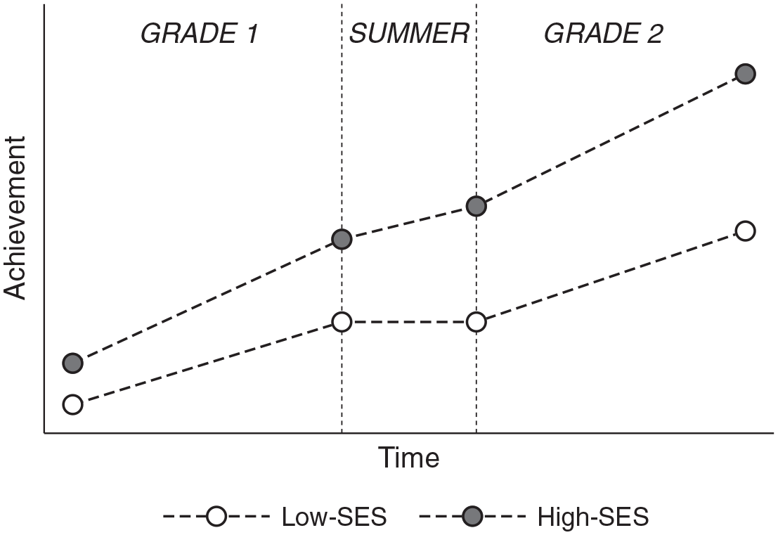
Seasonal Comparison Design: SES Inequality Increases Faster over the Summer Than during the School Year

Early SCD research in the United States consistently found SES inequality in learning increases faster in the summer than during the school year (e.g., Entwisle and Alexander 1992; Hayes and Grether 1983; Heyns 1978, 1987; Murnane 1975). These studies, now 40 years old, suggested that “when it comes to inequality by socioeconomic status, schools are more part of the solution than the problem” (Downey et al. 2004:616). In the 2000s, a second wave of studies refined the SCD to minimize bias arising from non-perfect overlap of test dates with the first and last days of the school years (Burkam et al. 2004; Downey et al. 2004). These works supported the earlier studies’ general conclusion of schooling effectively equalizing social gaps in learning.

Yet the consistent evidence from SCD research has recently been contested by critical replication studies. As von Hippel and Hamrock (2019) uncovered, findings of previous studies were driven by statistical artifacts related to seasonal change in the test-forms and noncomparable scaling of test-score data at various measurement occasions. Not all results and conclusions fell, however. When replicating the influential work of Downey and colleagues (2004) using newer data on multiple seasons (kindergarten, 1st grade, and 2nd grade) and properly scaled measures, von Hippel and colleagues (2018) found that although equalization effects of schooling were generally weak, schools did act as equalizing institutions in early life years. Findings from the replication study were consistent with the equalization hypothesis only when comparing learning rates by socioeconomic status during kindergarten and the summer gap before 1st grade (SES gaps shrunk in kindergarten but increased in the summer). After the first summer gap, findings did not support equalization (SES gaps remained constant during 1st grade, slightly decreased in the second summer gap, and remained constant again during 2nd grade; see von Hippel et al. 2018:341). However, even this recent replication suggests assertions that school is the culprit in socioeconomic inequality in learning are misguided. School compensation might be weaker than previously thought, and confined to children’s early years, but schooling does not seem to act as an institution that increases social inequality in achievement.

Issues related to the SCD go beyond statistical artifacts due to test form and scaling. One important assumption for the identification of school effects is the absence of schooling being the only reason for the change in learning during the summer. However, many things may occur during the summer that might be related to differential learning but unrelated to school absence. A second and rather practical restriction is the de facto limited applicability of the SCD outside the United States. National assessment studies consistently testing children twice a year over consecutive school years are scant in Europe and elsewhere. The limited cross-national applicability of the SCD is unfortunate, as cross-national differences in welfare regimes and education systems make general claims about school equalization highly uncertain. Finally, from an intervention perspective, the SCD translates to a particular treatment: closing the summer gap by extending the school year into the summer. However, reducing or abandoning summer holidays is but one of many possible interventions to increase school exposure.

The Differential Exposure Approach

A complementary strategy for studying the effect of school exposure on achievement entails contrasting achievement of children who were the exact same age at testing but experienced different amounts of schooling throughout their lives. This is the contrast constructed by our design, which has its roots in psychological research that aims at identifying the separate contribution of schooling and ageing to cognitive development (Carlsson et al. 2015; Cliffordson and Gustafsson 2008). Our approach also builds on Cornelissen and Dustmann (2019), who studied school-exposure effects by exploiting institutional rules that allowed children to enter the academic year at different terms in England. We focus on the effects of 1st-grade schooling but, in principle, the proposed approach may be extended to measure the exposure effect of later grades.

Ageing and exposure to schooling are perfectly colinear as children move through the school year: one additional month of schooling implies one additional month of age. Our design identifies the separate contribution of schooling and ageing to cognitive achievement by exploiting variations in birth dates and dates of test administration over the school year among children who entered 1st grade on the same calendar day.

Figure 2 illustrates the intuition behind the design. Panel A refers to fictional dates of birth (T_b), school start (T_s), and test administration (T_t) over calendar time. Imagine two children born three months apart but who started 1st grade on the same day—Peter and Simon. Due to the way the school system is organized, Simon was younger when he started school. Now imagine both Peter and Simon taking a cognitive test (resulting in a test score) on the same calendar day after six months in 1st grade. In this scenario, we would expect Simon to perform worse than Peter: even though they received the same amount of schooling, Simon was younger and likely at an earlier maturation point on the testing day. Now imagine a third child, Emily, who entered school with Peter and Simon. Emily also shares Simon’s birthday, which is exactly three months after Peter’s. However, for random reasons, Emily took the test exactly three months later in the school year. In this scenario, we would expect Emily to outperform Peter: even if they were the same age on the test day, Emily had received more schooling by then.

Figure 2.

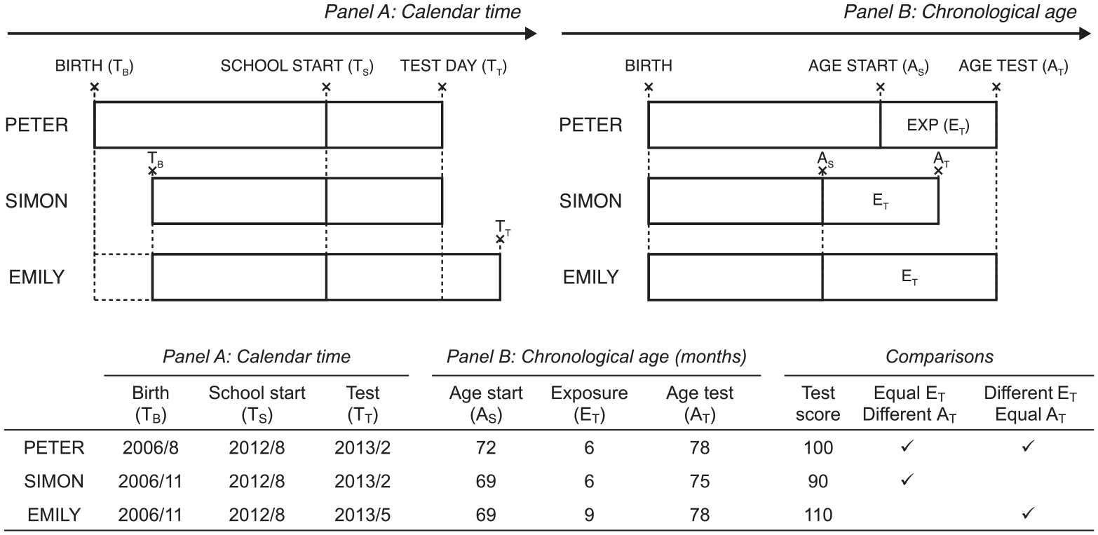
Illustration of the Core Elements of Our Design

Panel B of Figure 2 shows the same data over chronological age and makes it apparent that random variation in month of birth and test date, combined with a constant date of school start, allows us to separate the effects of ageing and schooling on learning. Comparing children who differed randomly in age (A_t) but had the same amount of school exposure (E_t) at the test day (i.e., Peter and Simon) yields information on the effect of age on achievement. Comparing children of the same age on the test day who randomly received a different amount of schooling up to that point (i.e., Peter and Emily) yields information on the contribution of schooling to achievement. More precisely, in our example, comparing Emily and Peter, who were the same age at the time of testing, provides us with an estimate for the effect of three-months difference in school-year exposure on achievement.

An important insight is that variations in age at test day and school exposure up to the test day leverage variations in the age at entry into 1st grade in our design. We could make sense of Simon’s lower performance compared to Peter as a direct consequence of the age difference at testing, yet Simon was younger at test day because he entered school at a younger age. In the same way, we could make sense of Emily’s better performance compared to Peter as a direct consequence of the additional schooling she received. However, Emily received additional schooling by the day of testing because she entered school at a younger age.

This discussion makes apparent that the effect of schooling measured by our design is a composite effect driven by differential exposure to schooling due to differential school-entry age. The manipulation of school exposure in our design is equivalent to replacing non-school time before school start with school time in a child’s lifespan. Most school systems feature fixed entry dates at the national or regional level combined with cut-off rules that lead to age-variations among children entering 1st grade on the same calendar day. Thus, considering such age-at-entry effects is essential to evaluate the effects of exposure to the school system. After all, one of the most straightforward real-world policies to increase early exposure to formal teaching in the classroom is to lower the school-entry age.

A Formal Illustration

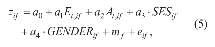
We can express the relationships more formally by the following model

$$y={\beta }_0+{\beta }_1{E}_t+{\beta }_2{A}_t+e,$$

(1)

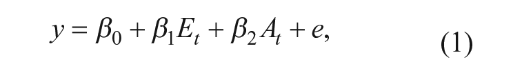
with y denoting student’s achievement, E_t denoting exposure to the school year up to the test date, A_t denoting age at test date, and e denoting a residual term. Age at test date is the difference between test date (T_t) and birth date (T_b). In most assessment data, school exposure can be measured by the time difference between the test date (T_t) and the starting date of school (T_s). Hence, E_t measures exposure to the school year including institutionally defined non-school time, such as hours spent at home after school, weekends, holidays within the academic term, and school absence due to illness.

To see why exposure coefficient β₁ (and age coefficient β₂) measure a composite effect, we follow Cornelissen and Dustmann (2019) and write out a theoretical model in which age at test day (A_t), age at entry (A_s), and school-year exposure (E_t) have separate effects on achievement:

$$y={\lambda }_0+{\lambda }_1{E}_t+{\lambda }_2{A}_t+{\lambda }_3{A}_s+e.$$

(2)

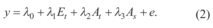
Because E_t = T_t – T_s, A_t = T_t – T_b, and A_s = T_s – T_b, it follows logically that A_s = A_t – E_t. Replacing A_s and rearranging terms leads to

$$\begin{array}{l}y={\lambda }_0+{\lambda }_1{E}_t+{\lambda }_2{A}_t+{\lambda }_3\left(A_t-E_t\right)+e\\ ={\lambda }_0+\left({\lambda }_1-{\lambda }_3\right)E_t+\left({\lambda }_2+{\lambda }_3\right)A_t+e,\end{array}$$

(3)

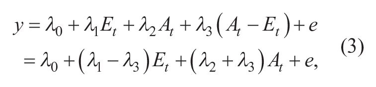
which demonstrates the composite nature of the school-exposure effect measure β₁ = λ₁ – λ₃ (as well as the age at test-date effect measured by β₂ = λ₂ + λ₃).

Some readers may be familiar with the long-standing debate over the age-period-cohort identification problem (Bell and Jones 2013). The theoretical model in Equation 2 involves the same problem because the three terms E_t, A_t, and A_s are mechanically related and, therefore, cannot be estimated in reality. Still, conditioning on two of the three components (as in Equation 1) yields a composite effect of E_t (β₁), which in our case is theoretically and practically meaningful. Considering achievement scores of a population of students who are the same age at test date (A_t), parameter β₁ identifies the expected marginal gain in achievement for the average student if the child had received more exposure to the school year, which in practice would have been feasible only by starting school earlier and substituting a period of “ageing outside school” with a period of “ageing in school.” Hence, β₁ reflects exactly the effect of increasing exposure to 1st grade (λ₁) obtained by starting school earlier in life (–λ₃, see also Cornelissen and Dustmann 2019). We thus deliberately conceive age-of-entry effects as a constituent part of the effects of schooling as they occur in an actual school system characterized by institutional rules of enrollment that feature age variations among children who start school on the same calendar day.

Note that parameters β₁ and β₂ sum to the learning rate over 1st-grade schooling (see the online supplement, Section A.1). Effectively, our strategy decomposes the learning rate into two hypothetical components: the effect of being one month older but not having one additional month of school exposure (β₂), and the effect of experiencing one additional month of school exposure but not being one month older (β₁).

To identify the model in Equation 1 in practical applications, we need sufficient variation in at least two of the three terms: test dates, T_t; dates of school-year start, T_s; and birth dates, T_b. In our empirical case, Germany, we will exploit variations in test dates and birth dates because school start is legally fixed and equal for all children (within states). If school start is fixed (i.e., T_s is a constant) and if test dates (T_t) and birth dates (T_b) are independent to observed and unobserved factors predicting achievement, then age at testing (A_t = T_t – T_b) and school exposure (E_t = T_t – T_s) are also independent of those factors. If these conditions are met, then our parameter of interest, composite effect β₁, can be estimated absent selection bias. This is but one application of the differential exposure approach. Other applications may draw on variation in birth dates and school start dates with fixed test dates or variation in school start dates and test dates combined with a fixed birth date. For example, Cornelissen and Dustmann (2019) exploited the fact that children in England enter the academic year at different terms (and thus have different school start dates).

Our analysis aims to test whether and how SES gaps in children’s achievement vary with school exposure. Hence, we model school-exposure effects as a function of the family’s socioeconomic status, which can be expressed by extending Equation 1 to include SES and the interaction terms with school exposure and age at test. After rearranging terms, we can write school and age effects as a function of SES:

$$\begin{array}{l}y={\beta }_0+\left({\beta }_1+{\beta }_4\cdot \mathrm{SES}\right)E_t\\ +\left({\beta }_2+{\beta }_5\cdot \mathrm{SES}\right)A_t+{\beta }_3\cdot \mathrm{SES}+e.\end{array}$$

(4)

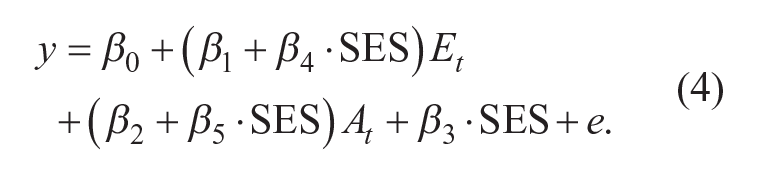
The model implies that the average SES gradient in 1st-grade achievement is a function of school exposure and age at test day (β₃ + β₄E_t + β₅A_t). Assuming the empirically likely scenario that children from higher-SES families show higher levels of achievement, on average, that is, (β₃ + β₄E_t + β₅A_t) > 0, we can derive three different theoretical scenarios regarding the effect of school exposure on achievement inequality by family SES: if β₄ < 0, expanding school exposure had an equalizing effect on SES-related inequality in achievement; if β₄ = 0, then school exposure had no effect on social gaps; and if β₄ > 0, school exposure exacerbated achievement inequality. Note that parameter β₄ captures the composite effect of differential school exposure achieved by leveraging school-entry age (for a formal demonstration, see the online supplement, Section A.2). The Methods section will provide more details on the precise estimation of the theoretical models described by Equations 1 and 4 in the context of our data.

Contribution of the Alternative Design

Our design enables research that complements the extant SCD research in important ways. First, our design features an internally valid estimate for the effect of school-year exposure as a dose-treatment among same-aged children. The design’s identification strategy rests on the exploitation of exogenous variations in exposure to the school year, which arise when sufficient exogenous variation is identified in either all three date variables—birth date, school-entry date, and test date—or, alternatively, in just two and the third one is fixed (i.e., a constant).

Second, our design adds a novel take on the role of schooling. From an intervention perspective, the design captures the effect of a treatment—having more schooling by starting earlier—which is different from the implicit treatment of the SCD—having more schooling by closing the summer gap between grades. The two designs would not necessarily yield the same findings, so they are complements. Much like the SCD, the DEA adds to an institutional perspective that conceives of schooling as more than simply providing instruction in the classroom, a conceptualization frequently found in economic perspectives that quantify school exposure by counting teaching hours or school and out-of-school days within the academic term (Carlsson et al. 2015; Cliffordson and Gustafsson 2008). An institutional perspective emphasizes the obvious fact that, once the transition to the school year is made, children’s daily lives and routines are socially clocked by the school system, including out-of-classroom learning during non-school days or hours within the academic term (e.g., on weekends, holidays, or when home after school). Schooling treatment in the DEA, as in the SCD, entails the compound exposure to the school year, including institutionally defined non-school periods within the academic term.

Third, our design has only modest data demands and requires only one test per child over the school year. This feature could help stimulate research on schooling effects in national contexts where high-quality seasonal data (like the ECLS-K in the United States) is just not available. In this article, we study the effect of schooling on socioeconomic inequality in learning in Germany, a national context of education and inequality in Europe that represents an excellent comparative case to the predominantly studied context of the United States.

Studying Effects of Primary Schooling in the German Context

Schools are embedded in the larger national context of inequality and education, and their equalization potential may vary as a function of institutional conditions. The parameters of the compensatory hypothesis—the social inequality of in-school versus out-of-school learning environments—provide a useful heuristic to understand why exposure to 1st-grade schooling may or may not equalize social gaps in children’s achievement in Germany.

Learning environments before school versus after the transition to school

Our study estimates a dose-treatment effect of schooling that substitutes time before school for time in primary school for a child of a given age: additional school exposure amounts to starting school earlier, which implies a crowding out of time spent in before-school environments by time spent in school environments. Hence, we would expect school exposure to lead to more equality if the learning environments children from different social backgrounds experience right before enrollment are more unequal than the learning environments they experience in primary schools.

Social inequality in German primary schools

The German education system is well-known for its stratifying effects due to rigid tracking at the transition to secondary education (age 10 to 11 in most German states). However, in contrast to many other countries, including the United States, primary education in Germany is highly standardized and centralized (by federal states) when it comes to grade curricula, organizational structures, and teachers’ qualifications (Allmendinger 1989). Teacher salaries in Germany rank among the highest in OECD countries, school autonomy and parental school choice is highly restricted, formal between- and within-school differentiation is absent, and private schools are rare and dependent on the states (OECD 2010). Moreover, primary school is compulsory, and attendance is enforced by law (even absenteeism of just one hour of instruction can bear legal consequences if unexcused). Highly standardized practices and administrative procedures not only foster uniform standards but are also likely to limit parental influence on school environments. Hence, compared to more “unequal” primary school systems in countries featuring lower levels of centralization, standardization, and regulation (e.g., the United States), primary schools in Germany may have a relatively high potential to compensate for social inequality in educational achievement.

Social inequality in before-school learning environments

Learning environments in primary schools are only one side of the coin, however. European countries are characterized by comparatively small socioeconomic inequality in living conditions compared to the United States (Gottschalk and Smeeding 2000; Smeeding and Rainwater 2004). Germany is no exception, featuring comparatively low wage inequality (Blau and Kahn 1996), low levels of residential segregation (Lichter, Parisi, and De Valk 2016), generous welfare state redistribution (Scruggs and Allan 2008), and tight institutional school-to-work linkages that are reflected in comparably stable and rewarding occupational careers for non-tertiary-educated workers (Kerckhoff 1995; Shavit and Muller 2000).

These arguments suggest comparably low social inequality in children’s home and neighborhood learning environments. However, homes and neighborhoods are not the only environments children experience before school enrollment in Germany. Publicly provided childcare and early-education centers also shape children’s early learning environments. Although not compulsory, kindergarten is nearly universally attended among children age 3 to 5 (92.2 percent in 2010, see German Federal Statistical Office 2011). German kindergarten is a welfare institution (part of child and youth welfare) that sees its primary purpose in minding and educating children. Kindergarten in Germany is not part of the education system: it offers care in a play-based setting absent formal curricula, and—in contrast to the U.S. concept of kindergarten—it does not entail any formal instruction (Linberg et al. 2019). As part of the welfare system, the provision of kindergarten rests on state-sponsored local initiatives (public and private). Nonetheless, there is some degree of standardization due to common federal standards (OECD 2015). Due to its high utilization rates amongpreschool-age children and the limited degree of differentiation, German kindergarten likely contributes to the equalization of learning opportunities right before children enter the school system.

Expectations

Given unequal out-of-school learning environments, the relatively low inequality of German primary schools may translate into a relatively large equalization potential (translating into β₄ < 0 in the context of our model, see Equation 4). Yet, Germany’s welfare state and the configuration of the preschool sector effectively compress social inequality in the learning environments children experience right before school, which, in turn, counteract primary schools’ equalization potential. It is therefore possible that school exposure does not equalize at all if social inequality of in-school environments simply mirrors social inequality in before-school environments (translating toβ₄ = 0). Our aim here is to empirically determine the outcome of the interplay of those mechanisms.

Data and Methods

Data

To study the effect of schooling on early achievement in Germany, we used nationally representative data from the kindergarten cohort of the German National Educational Panel Study (Blossfeld, Roßbach, and von Maurice 2011, data version 9.0.0). The kindergarten cohort covers a sample of children enrolled in kindergarten in 2010/2011, around age 4 to 5.

The sample was followed to the end of primary education (4th grade). Children were tested in various domains but only once in each grade. The original sample (N = 2,996) was augmented by a refreshment sample of 6,341 children in Wave 3 (2012/2013), which is the point marking the transition from kindergarten to primary education (1st grade).

For our purpose, that is, estimating the effect of 1st-grade school exposure, we drew on 1st-grade data (Wave 3). ¹ We selected 1st-graders from the refreshment sample because the original kindergarten sample suffered from strong attrition between the last year of kindergarten and 1st grade (approximately 85 percent attrition). The refreshment did not suffer from any attrition because it was sampled precisely in 1st grade (Wave 3, school year 2012/2013). Data collection involved child testing, parent interviews, and teacher and school headmaster questionnaires. Children were tested in school. There were two test booklets, one containing math and science tests and the other vocabulary and grammar tests. Testing took place on two test days at each school, and students worked on one test booklet per test day. ²

Schools were randomly assigned to two different time windows for testing: mid-February to mid-April 2013 (about 60 percent of students) versus mid-May to mid-June 2013 (about 40 percent). Consequently, testing commenced after the winter break and ceased before the summer break, when children had been in 1st grade for a minimum of approximately five months (February) and a maximum of approximately 10 months (June), respectively. The maximum variation in school exposure (at test day) induced by variation in testing dates was up to slightly more than five months of primary schooling, which is almost twice the length of school closures exploited by the SCD (three summer months approximately). Within the assigned time window, schools might have had some discretion in choosing the exact testing days, but the overall procedure ensured the timing of children’s testing was random. In fact, as we will show, neither parental SES nor school characteristics predict the days of testing. Parents of participating children were surveyed via telephone interview. Only one reporting parent (or the custodian in a few cases) was selected for interview.

Sample Selection

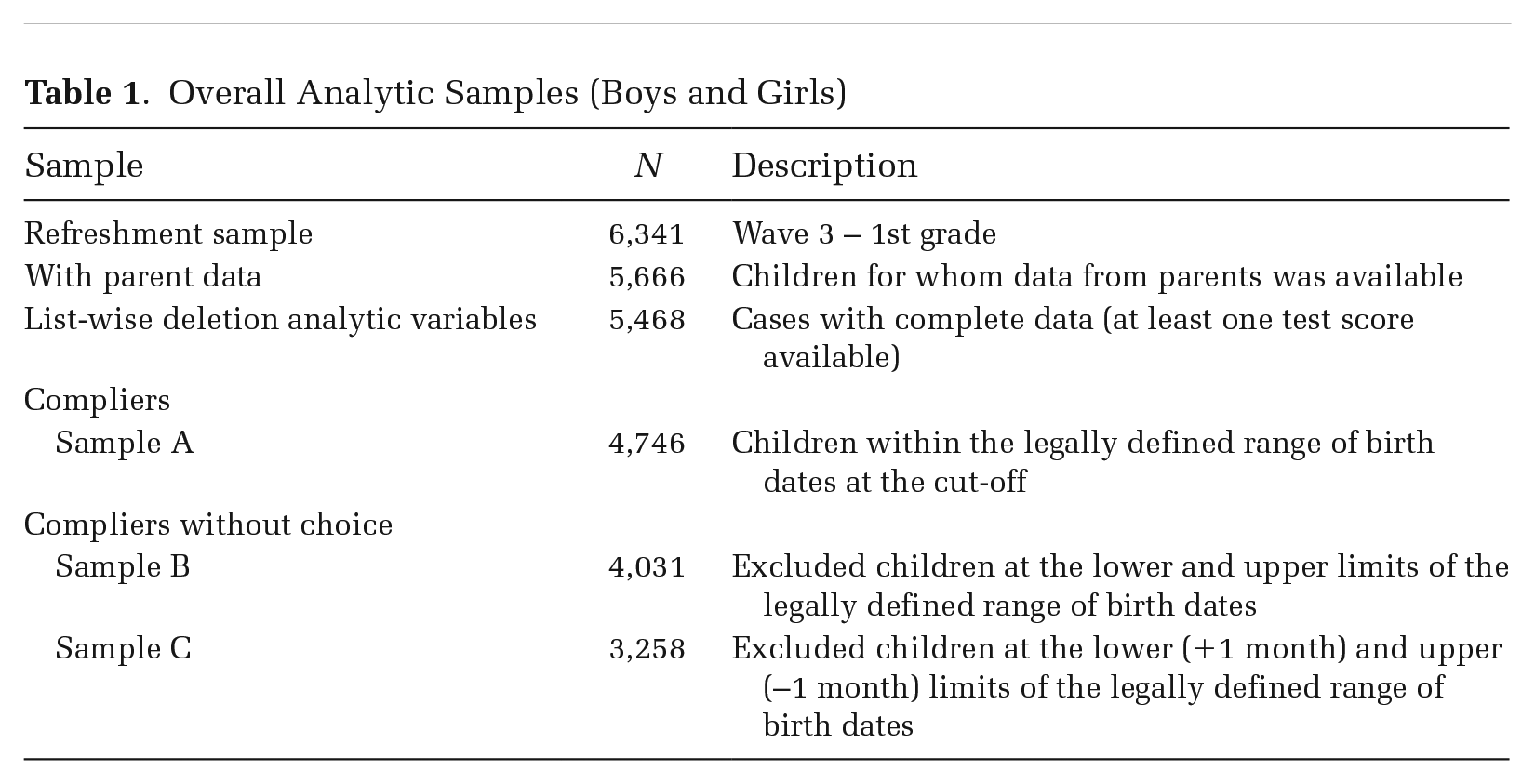
We selected children from the refreshment sample who participated in school testing and whose parents participated in the interview (see Table 1 for sample selection logic). After list-wise deletion of missing values on the main analytic variables, the sample included 5,468 children.

Table 1.

Overall Analytic Samples (Boys and Girls)

Sample	N	Description
Refreshment sample	6,341	Wave 3 – 1st grade
With parent data	5,666	Children for whom data from parents was available
List-wise deletion analytic variables	5,468	Cases with complete data (at least one test score available)
Compliers
Sample A	4,746	Children within the legally defined range of birth dates at the cut-off
Compliers without choice
Sample B	4,031	Excluded children at the lower and upper limits of the legally defined range of birth dates
Sample C	3,258	Excluded children at the lower (+1 month) and upper (–1 month) limits of the legally defined range of birth dates

In general, mandatory schooling in Germany (Vollzeitschulpflicht) commences in the calendar year children turn 6, if age 6 is reached before a certain cut-off date. If a child turns 6 after the cut-off, school enrollment happens in the subsequent year. Due to federal autonomy in German education, the exact cut-off date varies from end of June to end of September among federal states, and so does the exact day schools start (see Table 2). Cut-off dates are fixed within federal states. School start dates are also fixed within states, but they vary across academic years.

Table 2.

Legal Cut-Off Dates for Mandatory Schooling, School Start, and Definition of Complier Samples by Federal State

Federal State(German Laender)	Legal Cut-Off Date a	Start of School Year2012/2013 b	Compliers (Sample A)Born From/To	Compliers (Sample B)Born From/To	Compliers (Sample C)Born From/To
Baden-Wuerttemberg	Sept. 30	Sept. 10	Oct. 2005 – Sept. 2006	Nov. 2005 – Aug. 2006	Dec. 2005 – July 2006
Bavaria	Sept. 30	Sept. 13	Oct. 2005 – Sept. 2006	Nov. 2005 – Aug. 2006	Dec. 2005 – July 2006
Berlin	Sept. 30	Aug. 6	Oct. 2005 – Sept. 2006	Nov. 2005 – Aug. 2006	Dec. 2005 – July 2006
Brandenburg	Sept. 30	Aug. 6	Oct. 2005 – Sept. 2006	Nov. 2005 – Aug. 2006	Dec. 2005 – July 2006
Bremen	June 30	Sept. 3	July 2005 – June 2006	Aug. 2005 – May 2006	Sept. 2005 – April 2006
Hamburg	June 30	Aug. 2	July 2005 – June 2006	Aug. 2005 – May 2006	Sept. 2005 – April 2006
Hesse	June 30	Aug. 13	July 2005 – June 2006	Aug. 2005 – May 2006	Sept. 2005 – April 2006
Mecklenburg Western Pomerania	June 30	Aug. 6	July 2005 – June 2006	Aug. 2005 – May 2006	Sept. 2005 – April 2006
Lower Saxony	Sept. 30	Sept. 3	Oct. 2005 – Sept. 2006	Nov. 2005 – Aug. 2006	Dec. 2005 – July 2006
North Rhine-Westphalia	Sept. 30	Aug. 22	Oct. 2005 – Sept. 2006	Nov. 2005 – Aug. 2006	Dec. 2005 – July 2006
Rhineland-Palatinate	Aug. 31	Aug. 13	Sept. 2005 – Aug. 2006	Oct. 2005 – July 2006	Nov. 2005 – June 2006
Saarland	June 30	Aug. 15	July 2005 – June 2006	Aug. 2005 – May 2006	Sept. 2005 – April 2006
Saxony	June 30	Sept. 3	July 2005 – June 2006	Aug. 2005 – May 2006	Sept. 2005 – April 2006
Saxony-Anhalt	June 30	Sept. 6	July 2005 – June 2006	Aug. 2005 – May 2006	Sept. 2005 – April 2006
Schleswig-Holstein	June 30	Aug. 6	July 2005 – June 2006	Aug. 2005 – May 2006	Sept. 2005 – April 2006
Thuringia	Aug. 1 c	Sept. 3	Aug. 2005 – July 2006	Sept. 2005 – June 2006	Oct. 2005 – May 2006

a

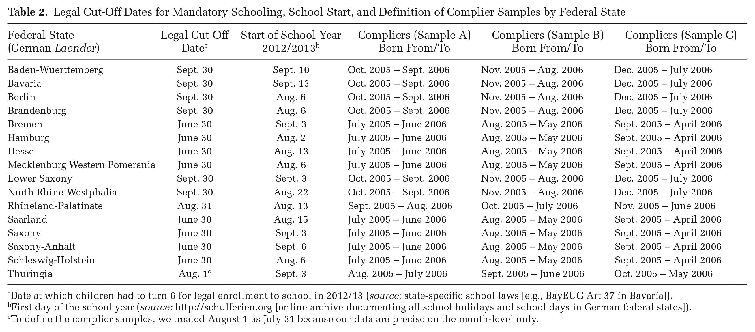
Date at which children had to turn 6 for legal enrollment to school in 2012/13 (source: state-specific school laws [e.g., BayEUG Art 37 in Bavaria]).

b

First day of the school year (source: http://schulferien.org [online archive documenting all school holidays and school days in German federal states]).

c

To define the complier samples, we treated August 1 as July 31 because our data are precise on the month-level only.

For example, in Bavaria, children born in September 2006 had to enter school on September 13, 2012 (school year 2012/2013), because they reached age 6 before the cut-off date (end of September). However, children born a year before, in September 2005, were scheduled to enter school in 2011 (school year 2011/2012). Finally, children born in October 2006 were scheduled to enter school in 2013 (school year 2013/2014). Parents can apply (but not choose) to defer or anticipate enrollment by one year, but there is no guarantee their application will be approved. Postponement is more regulated than anticipation; it is usually approved only if children are examined and determined to be physiologically, psychologically, or socio-emotionally unfit for school. In practice, parents generally only apply for anticipation or postponement when their children’s age at the cut-off date is close to the threshold; an overwhelming majority of children follow regular school enrollment. According to the German national education report for school year 2012/2013, about 10 percent of all school enrollments were irregular, with about 7 percent postponed enrollments and 3 percent anticipated enrollments (Hasselhorn et al. 2014).

Based on the cut-off dates, we derived the legally defined birth ranges corresponding to a compliant school enrollment in the academic year 2012/13 in each of the German Laender. For example, in Bavaria, all children born between October 2005 and September 2006 were in the “right” age range at the cut-off date and should have entered primary school on September 13, 2012. ³ Table 2 provides Laender details on cut-off dates, school start dates, and birth ranges corresponding to compliant school entry. Around 13 percent (unweighted) of the children in our sample were outside the right birth ranges and must have entered 1st grade in the fall of the previous (2011 or before) or following (2013 or after) years. Such unregular (early or late) school enrollment is likely associated with factors influencing achievement in school (e.g., children’s developmental stage or general school readiness). We excluded these noncompliers from the analyses because selectivity in age at entry would cause bias in our estimation of school-exposure effects.

The restriction to compliers implies our results are externally valid only for 1st-grade children who had a regular school enrollment. However, because 90 percent of school enrollments were regular in 2012/2013, our estimates are representative for the overwhelming majority of 1st-graders. Moreover, differences in compliance by family SES are minor in our data (see Tables F1 and F2 in the online supplement), and additional robustness analyses show our main results are not affected by potential selectivity of the complier samples (Figures E1 and E2 in the online supplement).

The sample of compliers (sample A, N = 4,746) includes only children whose age at school entry is defined entirely by the enrollment rules. Children who are just at or close to the upper and lower limits of the “right” birth range at the cut-off date are the most likely to apply for anticipation or postponement (Mühlenweg and Puhani 2010). For example, in Bavaria, a child age exactly 6 at the cut-off date (born September 2006) had the choice to apply for postponed enrollment in 2013/14 and be among the oldest rather than the youngest in the classroom. Conversely, a child age exactly 6 years and 11 months at the cut-off date (born October 2005) was only one month below the threshold age at the previous year’s cut-off and might have applied for anticipated enrollment in 2011/12; the child would then be the youngest rather than the oldest in the classroom. Compliers with the choice to apply for anticipation or deferral might be selective in terms of unobservable characteristics related to achievement, and their parents may have adopted strategic behaviors aimed at leveraging school-entry age (leading to endogeneity in our estimation).

To assess how robust our findings are against potential selectivity of these cases, we constructed alternative and stricter samples that removed from sample A potential compliers with the choice to apply for anticipation or deferral in progressive steps. First, sample B excludes children who were exactly at the lower (6 years) and upper (6 years and 11 months) limits of the “right” age range at the cut-off date (N = 4,031). For example, in Bavaria, sample B excludes children born in October 2005 and September 2006. Second, sample C additionally excludes children who were up to one month above (6 years and 1 month) or below (6 years and 10 months) the limits (N = 3,258). Thus, sample C is the strictest of all three samples. It aims to include only compliers without choice to apply for anticipation or deferral (i.e., the population of children for whom either anticipation or postponement of school entry is nearly absent). Sizes of the three samples vary slightly by outcome, as we aimed to maximize sample size for each outcome (see Table 3).

Table 3.

Distribution of Analytic Variables by Sample

	Sample A (Nmax = 4,746)				Sample B (Nmax = 4,031)				Sample C (Nmax = 3,258)
	M	SD	Min.	Max.	M	SD	Min.	Max.	M	SD	Min.	Max.
SES
Parental education	14.1	2.2	8.0	18.0	14.1	2.2	8.0	18.0	14.1	2.2	8.0	18.0
Parental ISEI a	51.4	18.4	11.6	89.0	51.6	18.5	11.6	88.7	51.8	18.4	11.6	88.7
Gender (1 = male, 2 = female)	1.5	.5	1.0	2.0	1.5	.5	1	2.0	1.5	.5	1.0	2.0
Grammar	(N = 4,487)				(N = 3,811)				(N = 3,070)
Score (WLE b score)	1.8	1.2	−4.6	5.9	1.8	1.2	−4.6	5.9	1.8	1.2	−4.6	5.9
Age at test (months)	85.0	3.9	77.1	95.1	85.0	3.4	78.1	94.1	84.9	2.9	79.1	93.0
School exposure (months)	7.2	1.5	5.1	10.4	7.2	1.5	5.1	10.4	7.2	1.5	5.1	10.4
Vocabulary	(N = 4,504)				(N = 3,827)				(N = 3,082)
Score (WLE b score)	1.5	.8	−2.3	5.1	1.5	.8	−2.3	5.1	1.5	.8	−2.3	5.1
Age at test (months)	85.0	3.9	77.1	95.1	85.0	3.4	78.1	94.1	84.9	2.9	79.1	93.0
School exposure (months)	7.2	1.5	5.1	10.4	7.2	1.5	5.1	10.4	7.2	1.5	5.1	10.4
Math	(N = 4,535)				(N = 3, 852)				(N = 3,112)
Score (WLE b score)	.1	1.1	−5.3	4.6	.1	1.1	−5.3	4.6	.1	1.1	−4.5	4.6
Age at test (months)	85.0	3.8	77.1	95.1	84.9	3.3	78.1	94.1	84.9	2.9	79.1	93.0
School exposure (months)	7.2	1.5	5.1	10.3	7.2	1.5	5.1	10.3	7.2	1.5	5.1	10.3
Science	(N = 4,536)				(N = 3,853)				(N = 3,113)
Score (WLE b score)	.1	.9	−2.8	4.1	.1	.9	−2.8	3.6	.1	.9	−2.8	3.6
Age at test (months)	85.0	3.8	77.1	95.1	84.9	3.3	78.1	94.1	84.9	2.9	79.1	93.0
School exposure (months)	7.2	1.5	5.1	10.3	7.2	1.5	5.1	10.3	7.2	1.5	5.1	10.3

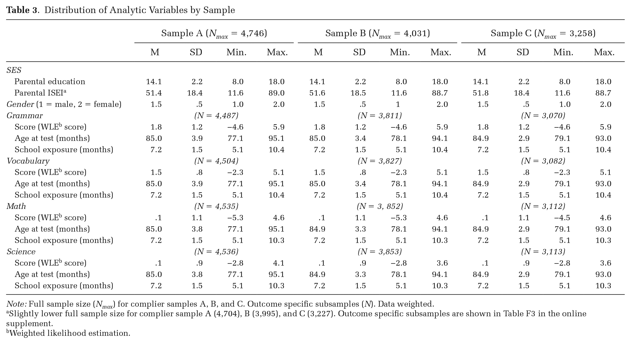
Note: Full sample size (N_max) for complier samples A, B, and C. Outcome specific subsamples (N). Data weighted.

a

Slightly lower full sample size for complier sample A (4,704), B (3,995), and C (3,227). Outcome specific subsamples are shown in Table F3 in the online supplement.

b

Weighted likelihood estimation.

Cognitive Outcomes

We examine school-exposure effects on children’s language competence (vocabulary and grammar), mathematical literacy, and scientific literacy. These cognitive domains are subject to learning in school and at home and were assessed for the 1st-grader sample as part of the general assessment framework of the NEPS (Artelt, Weinert, and Carstensen 2013). We give a brief overview of the NEPS testing here, and we provide more details in the online supplement, Section B.

The NEPS test frameworks for math and science are in line with national curriculum standards and the literacy concept adopted by the PISA studies. Scientific literacy encompasses knowledge of scientific concepts and facts as well as understanding of scientific processes (Hahn et al. 2013). Mathematical literacy entails knowledge of mathematical ideas and cognitive processes involved in solving math problems (Neumann et al. 2013). Receptive vocabulary captures lexical knowledge of words, and receptive grammar measures morphological-syntactical abilities related to the formation of words and sentences; both form the foundational dimensions of “academic” language as used in classroom instruction and textbooks (Berendes et al. 2013). Together, these test domains provide a good balance between more general language skills (vocabulary and grammar) and more curriculum-related skills (math and science), and between content knowledge and problem-solving skills. Test scores for all domains are scaled based on item-response theory (IRT) models that provide interval scaled scores (WLE scores) and best represent children’s abilities (Pohl and Carstensen 2012).

Table 3 describes test-score variables in the original metrics. For our analyses, we z-standardized test scores for all four domains in each sample to have a common mean of zero and unit standard deviation. Test-score reliability is .73, .74, and .87 for science, math, and vocabulary, respectively (no reliability data were available for grammar). Imperfect reliability inflates test-score variance, which can lead to attenuation bias in estimates for the effects of SES and schooling on z-scores. Thus, except for grammar, we adjusted test scores for reliability, as suggested in Reardon (2011). We comment on both the unadjusted and adjusted results.

School Exposure and Age at Testing

Exposure to 1st-grade schooling is exogenous only if test dates are independent of SES and other factors influencing achievement (because E_t = T_t – T_s with T_s being a constant for students from the same federal state). Test dates should fulfill such requirements by design, as schools were randomly assigned to testing periods and neither 1st-grade students nor their parents had any influence on the timing of tests. ⁴ We can be confident about exogeneity in test dates if test dates are not predicted by parental SES or school characteristics. Table 4 shows results from regression models that attempt to predict birth and test dates based on parental SES and class-level characteristics. Results clearly show that, within federal states, test dates are not predicted by SES nor a wide array of characteristics relating to the social, cognitive, and noncognitive composition of the classrooms and classroom quality and conditions. The independence between test dates and class characteristics is particularly reassuring because, although assigned to testing periods, schools might have had some discretion in choosing the exact testing dates (within periods).

Table 4.

Regression of Birth and Test Dates on Parental SES and Class-Level Characteristics

	Birth Date			Test Date a
	A	B	C	A	B	C
Student level
Parental education	.057 * (.027)	.044 (.024)	.021 (.022)	−.012 (.011)	−.017 (.012)	−.022 (.013)
Parental ISEI	.006 (.003)	.002 (.003)	.000 (.003)	−.001 (.001)	−.001 (.001)	−.001 (.002)
Class level b
Social composition
% Migrants	.000 (.003)	−.001 (.003)	−.001 (.003)	−.004 (.003)	−.004 (.003)	−.004 (.003)
% Low social class	−.005 (.004)	−.005 (.004)	−.003 (.003)	−.004 (.004)	−.004 (.004)	−.003 (.004)
% Parents high educ.	.004 (.005)	.008 (.004)	.006 (.003)	.000 (.004)	−.001 (.004)	−.001 (.004)
Cognitive skills c
Written language	−.028 (.084)	.014 (.075)	.001 (.067)	.064 (.080)	.081 (.081)	.073 (.084)
Oral language	.079 (.082)	.104 (.076)	.014 (.065)	.029 (.083)	.027 (.085)	.027 (.088)
Science	.071 (.084)	.034 (.081)	−.037 (.070)	.035 (.091)	.031 (.092)	.044 (.094)
Math	.062 (.102)	.074 (.094)	−.016 (.080)	.046 (.098)	.036 (.099)	.039 (.101)
Noncognitive skills
Social skills c	.059 (.076)	.111 (.070)	.095 (.066)	−.074 (.081)	−.093 (.079)	−.095 (.082)
Interested d	−.028 (.092)	.033 (.086)	.045 (.082)	.021 (.106)	.003 (.108)	−.007 (.111)
Autonomous d	.081 (.088)	.105 (.083)	.104 (.080)	.048 (.091)	.025 (.089)	.033 (.091)
Concentrated d	.034 (.086)	.035 (.082)	.033 (.075)	−.114 (.094)	−.128 (.094)	−.132 (.098)
Classroom size (m2) e	−.005 (.058)	.016 (.054)	.046 (.048)	−.002 (.059)	−.010 (.061)	−.016 (.061)
Quality of classroom f
Brightness	−.043 (.092)	−.034 (.083)	−.060 (.076)	−.133 (.093)	−.109 (.094)	−.099 (.096)
Size	.007 (.062)	.010 (.059)	.071 (.049)	−.098 (.074)	−.091 (.073)	−.076 (.074)
Functionality	.046 (.071)	.077 (.070)	.063 (.059)	−.064 (.086)	−.067 (.086)	−.052 (.088)
Structural integrity	.000 (.065)	.021 (.063)	−.005 (.057)	.014 (.076)	−.003 (.075)	.006 (.077)
Acoustics	−.101 (.064)	−.088 (.063)	−.035 (.056)	−.081 (.083)	−.054 (.082)	−.043 (.083)

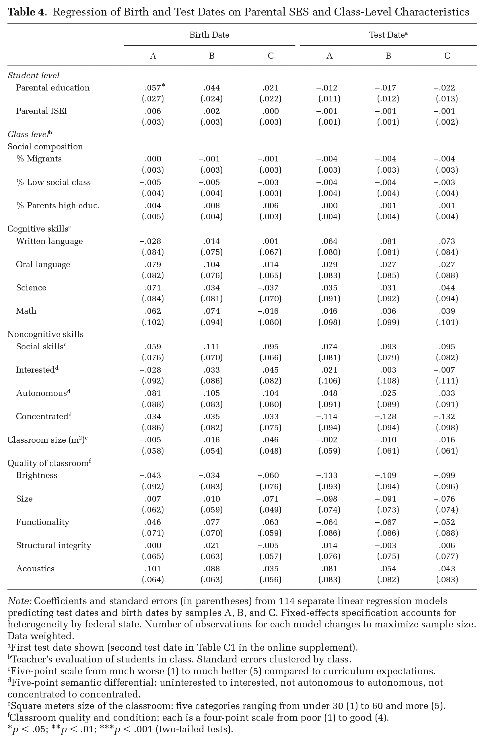
Note: Coefficients and standard errors (in parentheses) from 114 separate linear regression models predicting test dates and birth dates by samples A, B, and C. Fixed-effects specification accounts for heterogeneity by federal state. Number of observations for each model changes to maximize sample size. Data weighted.

a

First test date shown (second test date in Table C1 in the online supplement).

b

Teacher’s evaluation of students in class. Standard errors clustered by class.

c

Five-point scale from much worse (1) to much better (5) compared to curriculum expectations.

d

Five-point semantic differential: uninterested to interested, not autonomous to autonomous, not concentrated to concentrated.

e

Square meters size of the classroom: five categories ranging from under 30 (1) to 60 and more (5).

f

Classroom quality and condition; each is a four-point scale from poor (1) to good (4).

*

p < .05; ^**p < .01; ^***p < .001 (two-tailed tests).

In addition to random test dates, the exogeneity of age at the day of testing also requires birth dates to be independent of SES and other factors influencing achievement (because A_t = T_t – T_b). Birth dates should be exogenous in our samples because we only selected compliers with the enrollment rules implemented in each federal state. Table 4 shows this is largely the case in our three samples, with the partial exception of parental education in the overall sample of compliers (sample A). However, the association between parental education and birth date is trivial and, as expected, disappears when moving to the more restrictive samples of compliers without the choice to apply for anticipation or deferral (samples B and C).

Selectivity analyses in Table 4 make us confident that, within federal states, children in our samples randomly differed in school-entry age, which resulted in random variation in age at test and exposure to 1st-grade schooling. Interestingly, this was the case even in the overall sample of compliers (sample A), for which we might have expected larger SES-related age differences at school entry, possibly due to parental strategic behavior. Thus, we mainly comment on results for sample A, but we also report findings for more restrictive samples B and C.

Socioeconomic Status of the Family

We use parents’ education and occupational status as proxies for family SES. In Germany, formal educational attainment usually precedes childbirth and is comparably stable over the life course (Hullen 2001; Müller and Jacob 2008). Occupational status, in contrast, is subject to more fluctuations and is more prone to measurement error. Thus, we prefer parental education as our primary SES indicator.

We constructed the parental education measure by averaging the number of years necessary to attain parents’ educational certificates (see Skopek and Munz 2016). Family occupational status is measured by averaging the ISEI among parents (Ganzeboom and Treiman 1996). This information was provided by parent interviews in Wave 3 or recovered from later waves if missing (parental ISEI had slightly more missingness than parental education). We report the main analyses for parental education, but results using parental ISEI are very similar (see Figure D1 in the online supplement). Henceforth, we use parental education and SES synonymously. Descriptive statistics for all variables used in the main analyses are shown in Table 3. The analyses using ISEI involve minimally smaller samples because we aimed to maximize sample size for each SES indicator and outcome (see Table F3 in the online supplement).

Modeling Approach

Our modeling involves regressing test scores on school exposure while accounting for gender, age at test, and state fixed effects. The baseline estimation model resembles Equation 1:

$$\begin{array}{l}{z}_{if}=a_0+a_1{E}_{t,if}+a_2{A}_{t,if}+a_3\cdot SE{S}_{if}\\ +a_4\cdot GENDE{R}_{if}+m_f+e_{if},\end{array}$$

(5)

where the z-standardized test score of individual i in federal state f is regressed on gender, parental SES, age at testing (A_t), and exposure to 1st-grade schooling up to testing (E_t). The estimation model also includes fixed effects for German federal states (m_f). E_t is random only when children are subject to the same enrollment rules. Hence, accounting for state effects is necessary because cut-off dates and school start dates vary across German Laender.

Our main interest lies in studying if SES gaps in achievement decrease with exposure to 1st grade (keeping age at test constant). Modeling interaction terms in accordance with the theoretical model described by Equation 4 provides a direct test for this idea:

$$\begin{array}{l}{z}_{if}=b_0+b_1{E}_{t,if}+b_2{A}_{t,if}+b_3\cdot SE{S}_{if}\\ +b_4{E}_{t,if}\cdot SE{S}_{if}+b_5{A}_{t,if}\cdot SE{S}_{if}\\ +b_6\cdot GENDE{R}_{if}+m_f+e_{if}.\end{array}$$

(6)

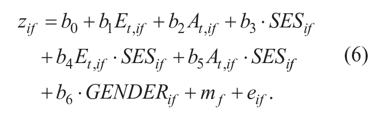
We estimated Equations 5 and 6 separately for each standardized competence measure and analytic sample (A, B, and C). Variables measuring age at test day, school exposure at test day, and SES are centered in each subsample to ease interpretation. Although we did not have a hypothesis on heterogeneity in schooling effects between boys and girls, we additionally estimated Equations 5 and 6 for boys and girls separately to explore the possibility of different schooling effects by gender. As a result, for the main analyses, we estimated 126 models for each of the two SES measures. We also ran a series of alternative models to ensure the robustness of our findings. All analyses used design weights provided by the NEPS.

Results

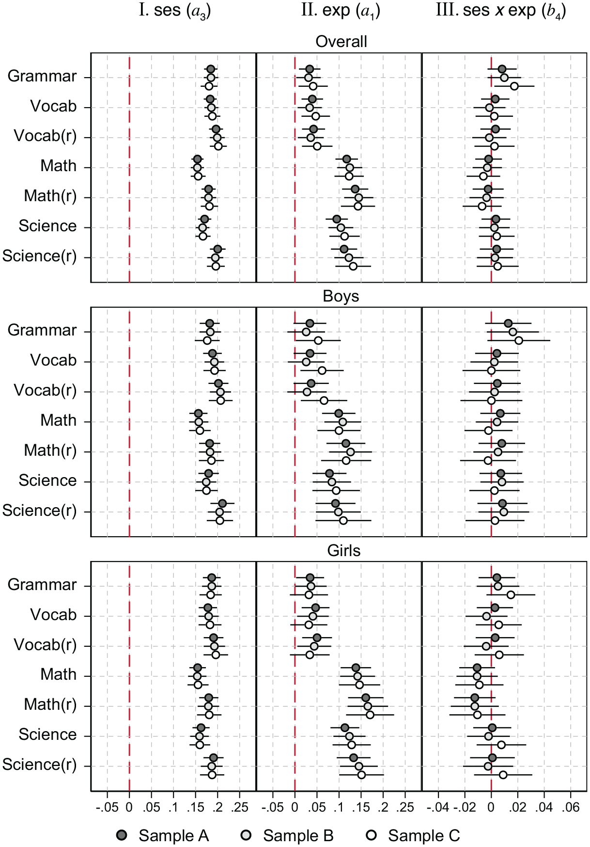
Tables 5 and 6 summarize the main estimates of our analysis obtained for sample A. We start with Table 5, presenting results from the baseline model (Equation 5) that estimates the main effects of school exposure, age at test, and years of parental education (noted by SES) while controlling for gender and federal-state differences (fixed effects). In line with previous studies on achievement gaps, our results show substantial SES gaps among children at the start of school. Coefficients of .15 to .20 imply a maximum gap of 2 standard deviations (SD) across the entire range of parental education (10 years of parental education). The gap is somewhat lower in math (.15) compared to grammar (.18), vocabulary (.18), and science (.17). As expected, reliability-adjusted scores (not available for grammar) reveal somewhat larger SES coefficients (.18 to .20). Overall, the SES–achievement association is substantial and, despite minor differences, consistent across domains. SES coefficients are plotted in the upper panel of Figure 3 (Column I); for comparison, the figure also shows coefficients obtained from the more restrictive complier samples B and C. SES gradients in the restricted samples are virtually identical to the overall complier sample A.

Table 5.

Baseline Models (Equation 5): Effects of Parental Education (SES), Age at Test Day, and School Exposure at Test Day on Standardized Test Scores (Sample A – Boys and Girls Jointly)

	Baseline Models (Equation 5)
		VOCAB.		MATH		SCIENCE
	GRAM.	Unadj.	Adj.	Unadj.	Adj.	Unadj.	Adj.
SES (parental ed.)	.184 *** (.008)	.183 *** (.008)	.196 *** (.008)	.154 *** (.007)	.180*** (.008)	.171*** (.008)	.200*** (.009)
School exp.	.033 ** (.012)	.039 ** (.012)	.042 ** (.013)	.117 *** (.013)	.137*** (.015)	.095*** (.013)	.111*** (.015)
Age (at test day)	.029 *** (.005)	.044 *** (.005)	.047 *** (.005)	.039 *** (.005)	.046*** (.005)	.037*** (.005)	.044*** (.006)
Constant	−.086 *** (.024)	.047 (.024)	.050 (.026)	.093 *** (.024)	.108*** (.028)	.017 (.024)	.020 (.029)
N	4,487	4,504		4,535		4,536
R 2	.223	.234		.216		.214

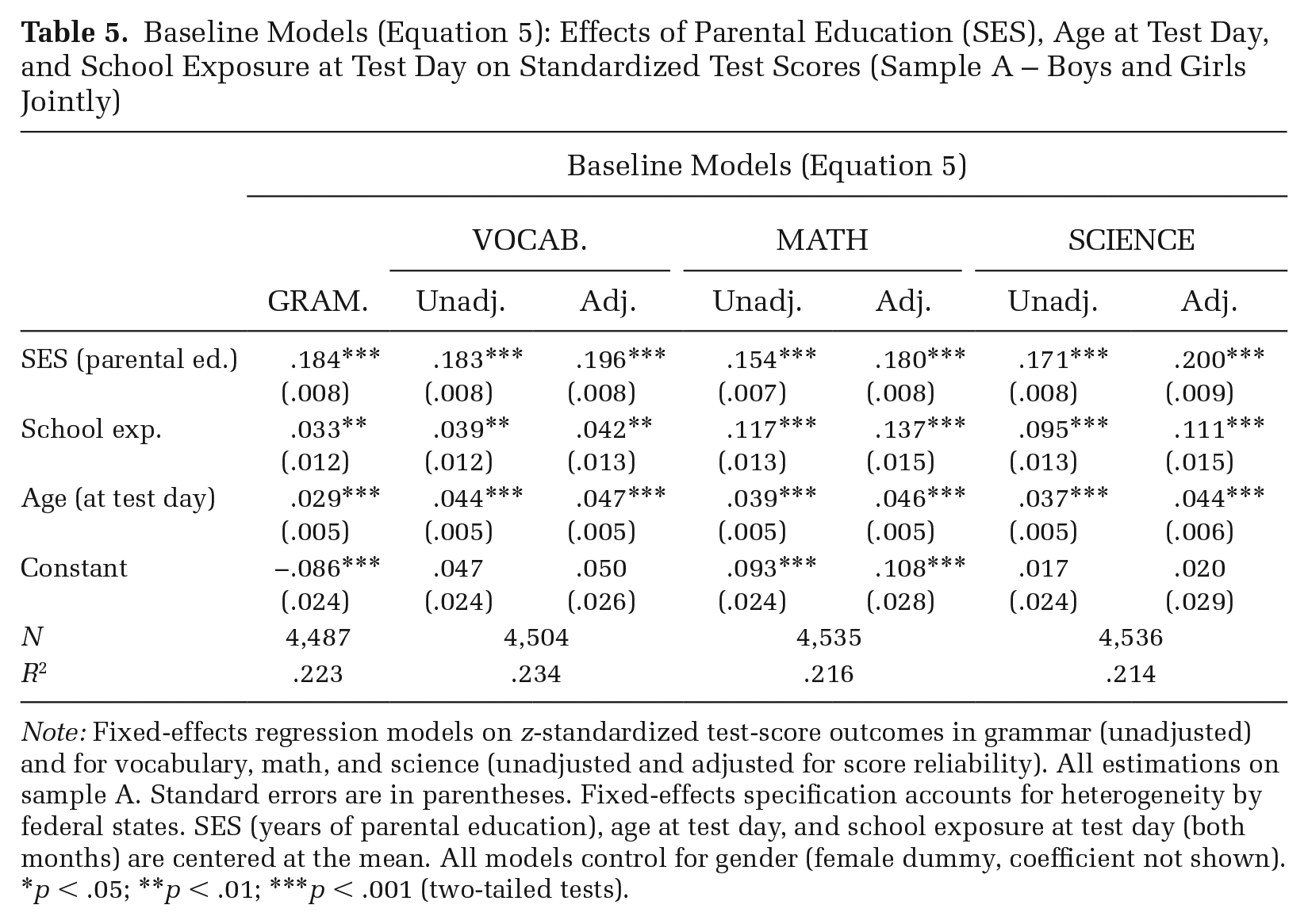
Note: Fixed-effects regression models on z-standardized test-score outcomes in grammar (unadjusted) and for vocabulary, math, and science (unadjusted and adjusted for score reliability). All estimations on sample A. Standard errors are in parentheses. Fixed-effects specification accounts for heterogeneity by federal states. SES (years of parental education), age at test day, and school exposure at test day (both months) are centered at the mean. All models control for gender (female dummy, coefficient not shown).

*

p < .05; ^**p < .01; ^***p < .001 (two-tailed tests).

Table 6.

Models with Interaction Terms (Equation 6): Effects of Parental Education (SES), Age at Test Day, and School Exposure at Test Day on Standardized Test Scores (Sample A – Boys and Girls Jointly)

	Models with Interaction Terms (Equation 6)
		VOCAB.		MATH		SCIENCE
	GRAM.	Unadj.	Adj.	Unadj.	Adj.	Unadj.	Adj.
SES (parental ed.)	.185 *** (.008)	.183 *** (.008)	.197 *** (.008)	.155 *** (.007)	.180*** (.008)	.172*** (.008)	.202*** (.009)
School exp.	.033 ** (.012)	.039 ** (.012)	.042 ** (.013)	.117 *** (.013)	.136*** (.015)	.094*** (.013)	.110*** (.015)
SES × School exp.	.008 (.006)	.003 (.005)	.003 (.006)	−.002 (.005)	−.002 (.006)	.003 (.006)	.004 (.007)
Age (at test day)	.029 *** (.005)	.044 *** (.005)	.047 *** (.005)	.039 *** (.005)	.046*** (.005)	.038*** (.005)	.044*** (.006)
SES × Age	−.001 (.002)	−.000 (.002)	−.000 (.002)	.003 (.002)	.004 (.002)	.006** (.002)	.008** (.003)
Constant	−.087 *** (.024)	.047 (.024)	.050 (.026)	.094 *** (.024)	.109*** (.028)	.019 (.025)	.022 (.029)
N	4,487	4,504		4,535		4,536
R 2	.223	.234		.216		.217

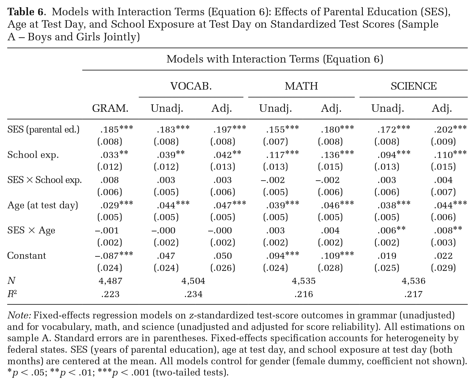
Note: Fixed-effects regression models on z-standardized test-score outcomes in grammar (unadjusted) and for vocabulary, math, and science (unadjusted and adjusted for score reliability). All estimations on sample A. Standard errors are in parentheses. Fixed-effects specification accounts for heterogeneity by federal states. SES (years of parental education), age at test day, and school exposure at test day (both months) are centered at the mean. All models control for gender (female dummy, coefficient not shown).

*

p < .05; ^**p < .01; ^***p < .001 (two-tailed tests).

Figure 3.

Effects of SES (Parental Education) and School Exposure (“Exp”) at Test Day on Cognitive Achievement

Table 5 also provides clear evidence for the positive effects of school exposure and age at test on child achievement. School effects are statistically significant across the board. Notably, schooling exposure has a larger effect on math and science than on vocabulary and grammar. For example, one additional month of schooling (without an additional month of age) increases math scores by about 12 percent of an SD (14 percent for reliability-adjusted scores), whereas it increases vocabulary scores only by 4 percent of an SD. In contrast to schooling effects, age effects are more similar across domains and, with respect to math and science, comparably smaller in size: one month of age (without an additional month of schooling) is associated with 3 to 5 percent of an SD higher scores. For vocabulary and grammar, age and school effects are nearly identical. Recall that school and age effects add up to children’s monthly learning rate over 1st-grade schooling. For example, based on our estimates, a child’s vocabulary score (unadjusted) is expected to increase by 83 percent of an SD after 10 months of being in 1st grade ([.039 + .044] × 10 = .83). Around half of that increase is explained by exposure to schooling (.039/ [.039 + .044] = .47). The equivalent for math (unadjusted) is a score growth by 1.6 SDs with schooling explaining three fourths of it. Figure 3 (upper panel, Column II) shows schooling effects are statistically identical across all samples (A, B, and C). The same holds for ageing effects (see Figure D2 in the online supplement).

What can explain our findings of domain-specific school-exposure effects? We argue that methodological differences between tests (e.g., test reliability, IRT scaling of a particular test) can be ruled out as an explanation for at least two reasons. First, results are very similar whether or not we adjust scores for reliability. Second, if methodological differences between tests were to cause differences in estimated schooling effects, we would expect ageing effects to vary accordingly. However, ageing effects are similar in all domains.

Having ruled out methodical artifacts, we can at this point only speculate on substantive explanations for why we find comparably smaller schooling effects on language-related domains. Like math and science content, vocabulary and grammar training form part of the 1st-grade curriculum (part of the subject “Deutsch,” in which children learn to read and write). However, because language learning is a very robust process that happens early in life (Shonkoff and Phillips 2000), language skills might be less malleable at later ages in school. Saturation effects may also play a role because language competencies are acquired long before school, whereas more technical math and science skills are typically learned in school. Further research may address these questions, but our findings do underline the importance of differentiating learning domains when examining schooling effects.

So far, our results have established positive effects of 1st-grade schooling on children’s learning. However, our main purpose was to test if schooling effects differ by parental SES. Table 6 shows results for our models that include interaction terms (see Equation 6). Figure 3 (upper panel, Column III) depicts interaction coefficients between school exposure and SES (interaction coefficients between age and SES are shown in Figure D2 in the online supplement). Interaction coefficients in Table 6 are negative (indicating equalization) only for the domain of math, although small. Only one of the 21 interaction coefficients (across outcomes and samples) reported in the upper panel of Figure 3 passes the test for statistical significance. ⁵ Hence, results regarding the SES–schooling interaction seem clear-cut: there is generally no meaningful interaction effect, implying schooling effects do not vary by parental SES. In other words, exposure to 1st-grade schooling does not seem to modify any of the SES gaps found in the various domains. This suggests all children—regardless of their parental background—benefit alike from schooling. ⁶

When it comes to the SES–age interaction, we find mixed evidence (see Table 6 and Figure D2 in the online supplement); although not statistically significant for vocabulary, grammar, and math, age effects seem to depend on SES for science. Estimates in Table 6 imply, for example, that the unadjusted SES gap in science between children differing in four years of parental education would have grown from approximately 69 to 93 percent of an SD over a 10-month period and independent of school exposure. ⁷ Hence, gaps in science by parental education might grow over 1st grade, but this seems due to factors related to age and not school exposure itself. Estimates for the stricter samples of compliers are almost identical (samples B and C).

We replicated all analyses using parental ISEI as a measure for SES. The main results are nearly identical to the ones reported here (see Figure D1 in the online supplement). We also tested for gender differences in the effects by running our models for boys and girls separately (middle and lower panels of Figure 3). In short, we could not detect meaningful differences in the inspected relationships by gender. Although there is somewhat more statistical uncertainty about the presence of schooling effects on grammar and vocabulary in the separated samples, our general conclusions about the absence of school-exposure effects on SES inequality apply to boys and girls equally. All in all, our results clearly suggest 1st-grade schooling did not reduce or increase SES inequality in educational achievement. School exposure did improve children’s learning in all skill domains, but it did not have any effect on SES-related inequalities in any of those domains.

Further Robustness Analyses

We ran additional analyses to ensure the robustness of our findings (see Figures E1 and E2 in the online supplement). First, even though being the overwhelming majority, compliers might not be a random subsample of all children entering 1st grade. Therefore, we replicated the main analyses accounting for potential selectivity of the complier samples via weighting (weights calculated by the inverse probability of being a complier estimated based on SES, early predictors of achievement, and federal state); this led to no different conclusions.

Second, we estimated our models including an indicator for migration background among the covariates (at least one parent not born in Germany) and, when relevant, the multiplicative terms between the migration indicator and school exposure and age at test. These augmented models may reflect sharper theoretical measures for SES inequalities, as migrant families are usually overrepresented in the lower tail of the SES distribution. Results from the augmented models fully confirm our general conclusions. As expected, SES gradients in achievement are somewhat lower compared to Figure 3, but social inequalities are still astoundingly strong and unchanged by school exposure.

We additionally estimated our models by grouping children in three (state-specific) groups that are equally spaced in terms of their age of entry into 1st grade (specifying entry age in a linear fashion would be inestimable, as discussed in the theoretical section). We interacted these entry-age dummies with SES when estimating interaction models. Estimation of school-exposure effects in these augmented models hinges on comparison among children with reduced variations in their entry age. This strategy also considerably reduces variation in school exposure by construction, and thus represents a strict test for our design. Adding entry-age dummies increases uncertainty around estimates of school-exposure effects, slightly reducing their magnitude, but leaves interaction terms with SES mostly unchanged. Hence, our general findings are supported by the data even when reducing variations in school-entry age and, therefore, exposure to 1st-grade schooling.

Conclusions

Decades of research has challenged the traditional sociological notion of schools as engines of social inequality in achievement and suggested that schooling acts as an institution ameliorating socioeconomic inequality in learning. Learning in home environments is so heavily dependent on parents’ socioeconomic position that even unequal school systems contribute to equalization. These ideas have received support from seasonal comparison studies that observe social gaps in achievement grow faster during the summer break—when schools are closed—compared to during the school year. Extant evidence, however, applies predominantly to the U.S. institutional context and leaves a gap of knowledge concerning other societies. Moreover, from an intervention perspective, the seasonal comparison design addresses a specific treatment in the form of absence of schooling during the summer break, which is not the only way to manipulate school exposure.

This study challenged the idea of schools as “equalizers” by examining if exposure to 1st-grade schooling reduced social inequality in learning outcomes in Germany. The equalizing potential of 1st-grade schooling is perhaps relevant in all institutional contexts but particularly in Germany, where significant school-tracking decisions are based on primary school achievement. If 1st-grade schooling reduces early achievement inequalities by social background, such an equalization effect would foster equal opportunities in track allocation, educational attainment, social mobility, and overall life-chances.

Drawing on related research in educational psychology and economics, we proposed a differential exposure approach (DEA) to identify causal effects of school exposure that exploits random variation of birth dates of children entering school on the same calendar day and variation in test dates of assessment studies. The proposed design has lower data demands compared to the SCD and relates to a different but complementary way to manipulate school exposure: extending school before school-life starts. We applied this design to recent educational data from the German National Educational Panel Study that tested 1st-grade students in a variety of cognitive domains.

Our findings are clear-cut. We found no effect of 1st-grade schooling on socioeconomic gaps in achievement in any skill domain. Gaps in achievement between same-aged children from higher versus lower social backgrounds were similar irrespective of the time children had been exposed to 1st-grade schooling. Even though we found clear evidence that schooling facilitates learning, our study did not find any systematic evidence that it does so to the advantage of children from high or low social backgrounds. Thus, we conclude that 1st-grade schooling in Germany neither equalizes nor exacerbates socioeconomic inequality in achievement. One can argue that schooling is beneficial for all children equally.

Our results challenge older findings from seasonal comparison studies that point toward equalizing effects of schooling in the United States, and they accord with more recent accounts that question those findings based on methodological shortcomings (von Hippel and Hamrock 2019; von Hippel et al. 2018). This study demonstrates that schooling does not always act as an institution ameliorating social inequality in learning. Prolonging the school year at the expense of the summer may decrease achievement inequality, but starting school earlier in life—an alternative policy to increase exposure to the school year—does not seem to create equalization. This finding calls for a more nuanced perspective on the role of schools in shaping socioeconomic inequalities in achievement. Policies that leverage school exposure in different ways (e.g., extending schooling in the early years of life as opposed to reducing summer breaks) may lead to substantively different results, and there is no guarantee they would all foster equalization. Yet, our findings add to a growing body of evidence that contradicts the notion that schools are a major source of achievement inequality, a notion that is still popular in many sociological narratives. As our data show, 1st-grade schooling may not compensate for social gaps in achievement, but it does not exacerbate them either.

A more nuanced perspective on the role of schooling would also benefit from considering the peculiarities of the institutional context in which schools operate. The strong standardization of Germany’s primary school system clashes with the absence of 1st-grade equalization we found. How can equal primary schools fail at fostering social equality in learning? At first, we may be tempted to search for the reasons behind the absence of school equalization in the organization and structure of the school system, but perhaps we should be looking outside the school system. German kindergartens and other welfare institutions limit social inequality in the learning environments before school entry and may well explain the absence of 1st-grade equalization. German primary schools are embedded in comparatively “not so unequal” out-of-school environments, which may itself bring school equalization to a halt. SCD research in the United States underlines how even unequal schools may equalize social inequality in learning. Our analyses of 1st-grade students in Germany show that even relatively equal school systems may not guarantee equalization.

What would it look like had we applied our design to 1st-grade students in the United States? A tentative, speculative answer cannot ignore the nature of the counterfactual before-school environments in the U.S. context. Unlike German kindergarten’s care and play focus, U.S. kindergartens are diversified schooling institutions that may be prone to exploitation by advantaged families. In the context of stronger inequality in before-school environments, we would expect primary school to contribute to equalization. However, not only kindergartens but also primary schools are more unequal in the United States compared to Germany. These facts may suggest that substituting unequal kindergartens with similarly unequal primary schools may not bear any consequences for socioeconomic gaps in learning. Still, swapping time spent in even more unequal environments before kindergarten with kindergarten might contribute to equalization. Our findings may inspire future studies trying to answer crucial questions about school equalization in early years in the United States and elsewhere.

Future research could also try to expand the theoretical model underlying previous seasonal comparison research. Attempts in that direction could depart from more formalized counterfactual models of schooling, as elaborated by Raudenbush and Eschmann (2015). Their model posits that equalization of learning environments does not translate mechanically into equalization of learning outcomes. Unequal learning gains from instructional inputs may offset benefits from more equal inputs. This would be the case, for example, if socially advantaged children have better skills, on average, and skill gains from instructional inputs are a positive function of previous skill levels (Cunha and Heckman 2008). Because social gaps in achievement are sizable before and right at the start of school in Germany (Linberg et al. 2019; Passaretta et al. 2020; Skopek and Passaretta 2021), a skill-begets-skill mechanism may give rise to unequal gains from schooling, and thus possibly provides an alternative explanation for the absence of school equalization effects.

So, does schooling decrease socioeconomic inequality in learning? We believe that finding simple, univocal answers to this question is a chimera. School equalization rests on out-of-school counterfactuals, and the variety of policies aimed at increasing the time children spend in school may not always foster equalization. Our study may help reframe the debate on the role of schooling for learning inequality by drawing attention to the different consequences of complementary ways of increasing children’s exposure to the school system. Still, the same policy may foster equalization in some countries but not others. These arguments point toward the embeddedness of schools in the broader societal context of social stratification and the importance that schools might have at different moments of children’s lives.

Schools are never “equalizers” per se, as equalization depends on specific out-of-school counterfactuals that vary across institutional, geographic, and temporal (e.g., lifecycle) contexts. The Coleman report in the early 1960s stressed the greater importance of non-school factors compared to school factors in shaping social gaps in achievement. Starting from the 1960s, seasonal design research has substantiated such a perspective and repeatedly argues that “when it comes to inequality by socioeconomic status, schools are more part of the solution than the problem” (Downey and colleagues 2004:616). Most recent studies have been skeptical of those earlier assertions. Our study substantiates such skepticism and challenges over-optimistic ideas about schooling as being always and unequivocally a social “equalizer”: rather, we point to the possibility that, depending on the circumstances, schools might have no consequences for social inequality in achievement.

Supplemental Material

sj-pdf-1-asr-10.1177_00031224211049188 – Supplemental material for Does Schooling Decrease Socioeconomic Inequality in Early Achievement? A Differential Exposure Approach

Supplemental material, sj-pdf-1-asr-10.1177_00031224211049188 for Does Schooling Decrease Socioeconomic Inequality in Early Achievement? A Differential Exposure Approach by Giampiero Passaretta and Jan Skopek in American Sociological Review