Sage Journals: Discover world-class research

Abstract

Behavioral science demands skillful experimentation and high-quality data that are typically gathered in person. However, the COVID-19 pandemic forced many behavioral research laboratories to close. Thankfully, new tools for conducting online experiments allow researchers to elicit psychological responses and gather behavioral data with unprecedented precision. It is now possible to quickly conduct large-scale high-quality behavioral experiments online, even for studies designed to generate data necessary for complex computational models. However, these techniques require new skills that might be unfamiliar to behavioral researchers who are more familiar with laboratory-based experimentation. We present a detailed tutorial introducing an end-to-end build of an online experimental pipeline and corresponding data analysis. We provide an example study investigating people’s media preferences using drift-diffusion modeling (DDM), paying particular attention to potential issues that come with online behavioral experimentation. This tutorial includes sample data and code for conducting and analyzing DDM data gathered in an online experiment, thereby mitigating the extent to which researchers must reinvent the wheel.

Keywords

online behavioral experiments PsychoJS drift-diffusion model computational modeling open science COVID-19

Behavioral experimentation methods are usually practiced in laboratory-based settings due to a need for highly accurate measurement hardware and software deployed in a highly controlled environment. Laboratory-based experiments maximize internal validity and experimental control but come with the cost of relatively small samples, high labor effort, and slow data collection times (for a review; Birnbaum, 2004). During the COVID-19 pandemic, many in-person behavioral experiment laboratories were shuttered. Thankfully, web-based solutions allowed behavioral research to continue. Today, even as opportunities for in-person data collection resume, researchers may wish to continue online behavioral experimentation. Online behavioral experimentation allows researchers to collect recorded behavioral data in programmed tasks, such as sequences of perceptual or preferential selection of choices (Anwyl-Irvine et al., 2020), logged mouse-tracking trajectories (Schoemann et al., 2021), and response time (RT) for message processing (Wilcox et al., 2021) or decision-making (Ratcliff & Hendrickson, 2021). Thus, online behavioral experimentation enables complex experimental designs and statistical modeling to examine within-subject and between-subject variation in subjects’ behavioral tendencies and cognitive processing, such as executive function, working memory, and decision-making. In addition, the declarative data from retrospective online survey studies have been challenged for the measurement discrepancy between self-reported behavior and people’s actual real-life behaviors, which questions the validity of only using self-report survey data as cognitive or behavioral indicators (Parry et al., 2021). Thus, online behavioral experimentation should be considered an important complement to survey-based methods to reveal people’s behavioral patterns and underlying cognitive processes (Hainmueller et al., 2015).

In fact, there are multiple benefits of online behavioral experimentation. First, it speeds up the data collection process significantly (Barbosa et al., 2022). Second, it enables more diverse large-scale participant samples. Instead of requiring participants to come in person to the laboratory, which often limits studies to convenience samples of undergraduate students, online experiments can reach large national or international participant samples, thereby increasing generalizability, and statistical power, and making it more feasible to engage in subgroup analysis. Finally, online experiments are highly compatible with open science practices (Dienlin et al., 2021). For example, online behavioral experimentation platforms such as Pavlovia (https://pavlovia.org/) provide hosting and code version control, which can easily be used in preregistrations and materials sharing. These practices increase research transparency, reproducibility, and replicability. Evidence is accumulating to show the validity and accuracy of online behavioral experimentation data, which showed high replicability of bringing offline laboratory-based results online (Bridges et al., 2020; Ratcliff & Hendrickson, 2021). Thus, we expect the adoption of online experimentation methods will benefit behavioral scientists in a wide range of research fields, such as cognitive psychology, behavioral economics, computational social science, and communication.

Online behavioral experiments also come with several potential challenges, such as potentially impaired data quality (Clifford & Jerit, 2014) and increased technical complexity (Reips, 2002). Here, we introduce a pipeline for building a web-based behavioral experiment for conducting a decision-making study using drift-diffusion modeling (DDM; Ratcliff & McKoon, 2008). We break the process down into a series of seven steps, beginning with hypothesis formation and concluding with model interpretation and including code for conducting an online DDM study and analyzing the data.¹ We conclude with a discussion of methods for addressing data quality and issues associated with online experimental designs. In what follows, we briefly introduce DDM before explaining its application in online experiments.

Behavioral Modeling

One key component in behavioral experimentation is the analysis of collected behavioral response data, such as choices and RTs. Modeling of behavioral response data usually requires a hypothetical cognitive mechanism of the behavior-generating process, in this example, a decision-making process. This unobservable cognitive decision-making process governs participants’ behaviors in the experimental paradigm and produces observable behavioral data, which needs appropriate computational modeling approaches to reveal the latent decision-making mechanism. Eventually, the cognitive decision-making process helps researchers to answer a wide range of research questions, including but not limited to consumption preferences or perceptual judgment of different stimuli (Milosavljevic et al., 2010), the impact of individual differences or experimental conditions on the decision-making process (Kowalczyk & Grange, 2020), the underlying driving forces of people’s real-world judgments and behaviors such as sharing of misinformation (Lin et al., 2023), and so on.

There are several benefits to behavioral modeling over alternative ways, such as survey-measured behavioral indicators or frequency-measured behavioral indices. To demonstrate, consider a researcher who is interested in studying why a person selects one type of media content over another. Most of the research in this area usually asks participants to report their media usage in a retrospective questionnaire or directly observes participant media choices without measuring RTs (Hartmann, 2009). However, these methods often fail to reveal the psychological processes driving selection, or why one type of media content is preferred over another (Knobloch-Westerwick, 2014), or fail to model stochasticity in choices independently from media preference (Alós-Ferrer et al., 2021). Computational behavioral models can overcome these limitations. Compared to statistical models of behavior, computational models provide a better sense of trial-level behavioral data (Wilson & Collins, 2019), richer explanatory power for the psychological processes that govern decision-making, as well as better predictive inference (Clithero, 2018).

Another benefit is that computational models are often more statistically powerful than frequency-based inference by accounting for the multi-modal behavioral variation of choices and RTs at trial, subject, and group levels (Stafford et al., 2020). For instance, a simulated RT and choice dataset (N = 200) shows that one class of computational decision-making models, the hierarchical Bayesian DDM (Ratcliff & McKoon, 2008; Wiecki et al., 2013), has higher power to detect preferences (Supplemental Figure S1A).² Across different model parameters, DDM has higher power compared to a choice model using only choice frequencies (Supplemental Figure S1B).

A related concern is that frequency-based inference potentially introduces bias to hypothesis testing. People’s decision-making is a time-consuming and multi-stage process (Ratcliff & McKoon, 2008). During different stages, the decision-maker develops distinct reasonings and biases which combine together to produce the final decision and execute the observed behavioral outcomes. However, a simplified and incomplete analysis of the behavioral outcomes, for example, frequency-based inference, takes a holistic view of the decision-making process, thus ignoring the decision biases developed in the initial stages of the decision-making. Consider a horror movie fan deciding between watching a horror movie and a comedy movie. The decision-making process might start with a bias against horror movies due to emotional avoidance but eventually shift toward watching horror movies due to curiosity needs. In short, a biased starting point away from the favored option will introduce the type II error, and a biased starting point near the favored option will introduce the type I error. Computational models can account for this by modeling bias, whereas this bias is not accounted for with frequency-based approaches. In sum, when compared to frequency-based methods, behavioral modeling offers more explanatory and statistical power.

The Drift Diffusion Model

DDM³ (Ratcliff & McKoon, 2008), under Decision Theory (Dayan & Daw, 2008), is one type of sequential sampling model (SSM), which offers a theoretical account of how people decide among two or more options. SSMs (Ratcliff & McKoon, 2008) are a class of computational decision-making models that account for people’s choices and reaction time. SSMs treat decision-making as a process where decision-makers sample option-favoring evidence and accumulate evidence to reach a decision threshold. In the current manuscript, we focus on the DDM for decision-making studies.

DDM was initially developed to explain several characteristics commonly observed in perceptual and memory-based decision-making tasks, including right-skewed RT distributions, correct versus error choice frequencies, and the speed-accuracy trade-off phenomenon (Ratcliff & McKoon, 2008). Later, studies found that DDM can be utilized to explain a range of decision-making processes, such as value-based consumption decisions (Milosavljevic et al., 2010), social decisions (Klauer et al., 2007), and reinforcement learning processes (Ratcliff & Frank, 2012). In addition, recent studies found DDM can be linked to neural signals, such as neural firing rate (Smith & Ratcliff, 2004), electroencephalography (EEG) signals (Ratcliff et al., 2009), and functional magnetic resonance imaging signals (Bode et al., 2012). This evidence indicates that DDM is a good algorithmic approximation of the actual decision-making processes implemented by our brains.

DDM suggests people’s decision-making is an evidence or information accumulation process with a constant drifting rate (Figure 1). Formally, for a two-choice value-based decision process, the two options are represented by two decision boundaries with the higher-value option as the upper boundary (a) and the lower-value option as the lower boundary (0). The decision-making process will start from a starting point in the middle of the two decision boundaries with or without preexisting decision bias (z) favoring either option. Then, for each time step, the decision process will stochastically move upward to the upper boundary (higher-value option) or move down to the lower boundary (lower-value option) with a constant drifting rate (v) with random noise. When the random walk reaches either one of the boundaries, the decision process is complete and ready to be executed. The DDM also includes a non-decision time (T) parameter and three variance parameters to account for the inter-trial variability of the decision process (Ratcliff et al., 2016).

Figure 1.

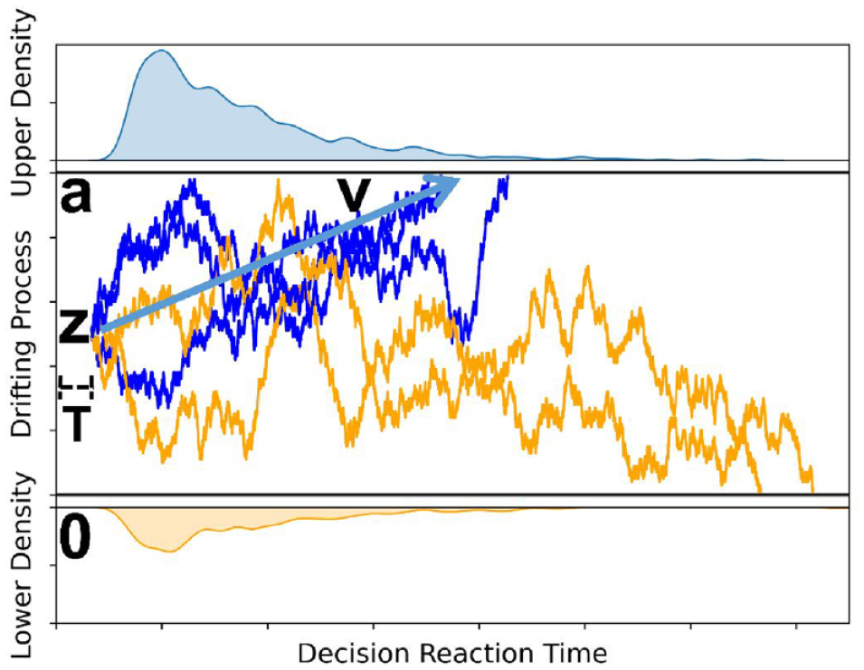
The DDM. The upper blue distribution is the observed decision RT for the higher-value option (upper boundary) chosen, and the lower orange distribution is the observed decision RT for the lower-value option (lower boundary) chosen.

The four computational parameters (v, a, T, and Z) have unique conceptual operationalizations in a decision-making context. Non-decision time (T) encodes people’s perceptual processing and representation of options as well as the time spent executing a decision (e.g., clicking a button to make a decision). The length of the non-decision time depends on the complexity of the presentation of options. For instance, image presentations would require shorter perceptual processing compared to text presentations. This is because it should take longer to read a body of text compared to looking at an image.

Decision boundaries (a, 0) account for people’s decision cautiousness with wider decision boundaries (i.e., a larger difference between a and 0) representing stronger caution in the decision-making process. More specifically, this parameter indexes the speed/accuracy trade-off where a wider boundary represents slower, more cautious, and therefore, more accurate decision-making, whereas a narrower boundary represents the opposite.

Decision starting point (Z) accounts for people’s decision bias that is unrelated to the valuation of the options itself. Bias might be driven by people’s ongoing preferences or non-choice characteristics. For instance, position order biases people’s choice of web page selection for search engine results (Craswell et al., 2008) and people’s decision to click on an advertisement (Agarwal et al., 2011) is biased by the position of the content.

Finally, drift rate (v) accounts for the rate of evidence accumulation. Some decisions may have an objectively correct option, as in a Stroop task. In such cases, the drift rate accounts for the evidence participants collect to determine the objectively correct option. By comparison, during value-based decision-making, the evidence being accumulated is the value differences between the given options (Milosavljevic et al., 2010). When the difference between the two options is small, the evidence accumulation process will be slow; thus, the drift rate will be small in magnitude and people’s choices will approach chance. By comparison, as the difference between two choices increases, the evidence accumulation process will be fast, the drift rate will be large in magnitude, and people’s choices will show a clear preference for one choice over the other.

A unique set of DDM decision parameters will result in different reaction time distributions and choice frequencies (Ratcliff & McKoon, 2008). For instance, while keeping the drift rate and decision starting point constant, increasing the decision boundary will spread and slow down RTs and increase the proportion of choices for the objectively correct or higher-value option (Supplemental Figure S2A). On the other hand, increasing only the drift rate will speed up RTs and increase the proportion of choices choosing the higher-value option. Importantly, and unlike the impact of the decision boundary, changes in drift rate have a stronger impact on the tail of the distribution (0.9 quantiles) compared to the leading edge (0.1 quantiles) of the distribution (Ratcliff & McKoon, 2008; Supplemental Figure S2B). Distinct from decision boundary and drift rate, changes in decision bias will lead to a shifting of the RT distribution toward the biased decision option (shorter RT for the biased option and longer RT for the other option) and a dramatic influence on the proportions of choices (Supplemental Figure S2C). Finally, non-decision time does not influence the proportion of choices or the shape of the RT distribution, but only the length of RT in a way that increasing non-decision time will lead to the increase of RT of the same amount value.

Challenges of Moving DDM Online

Several issues emerge from the application of DDM in online experimentation approaches. First, DDM is a complex behavioral model with a relatively large number of specified parameters. Thus, analyzing the complete set of parameters usually comes with computational difficulties, especially when the sample size is large (as is common with online experiments). Moreover, not all DDM parameters are of interest to every research question. For instance, non-decision time might not be of interest to research investigating people’s consumption preferences for media content with different attributes. Similarly, inter-trial variability parameters might not be of interest in studies examining individual or group-level differences in decision-making processes. As a result, researchers need to balance the parsimony and the completeness of DDM (Lerche & Voss, 2016).

Second, DDM fits RTs and choice data gathered in well-controlled simple two-option decision tasks, which often have limited external validity. Real-life decisions usually include multiple options rather than two options, are often not made repeatedly with the assumption of independence between each choice, and are usually not speeded. Thus, researchers need to take special care in designing their decision tasks and creating stimuli to simulate real-life decision scenarios.

Finally, to maximize the accuracy of model parameter estimation, DDM requires a large number of decision trials in experiments which brings practical difficulties for online experimentation due to concerns of participant motivation, distraction, fatigue, and other data quality issues.

An End-to-End Pipeline for Conducting and Analyzing an Online DDM Experiment

We aim to introduce a step-by-step tutorial for applying DDM in an online experiment. Our examples are specific to fitting a hierarchical Bayesian DDM using the hierarchical drift-diffusion model (HDDM) package for Python (Wiecki et al., 2013), but have similar applicability to other DDM estimation approaches, noting that alternative estimation approaches often come with additional assumptions that might differ from those specific to HDDM. To conduct an online DDM experiment, we need to design a two-option decision task that collects choice and RT data. Generally, there are five steps to designing the two-option decision task experiment and two steps to conducting the experiment and analyzing the data.

Step One: Hypothesis Formation

The first step is to characterize the decision problem based on research objectives. In this step, researchers need to analyze the decision problem in real life and conceptualize it at an abstract level. In this example, we consider why people might choose one type of media content over another. Researchers need hypotheses about (1) what drives people to make such media decisions (e.g., entertainment, information); (2) what are the decision options (e.g., movies, videos, news articles); (3) how are options presented (e.g., movie poster images, textual plot summaries, video trailers); (4) what attributes shape people’s choice (e.g., affect, novelty, social factors); (5) at which level are the attributes evaluated (e.g., habitual, goal oriented); (6) what are the potential gains (e.g., enjoyment, curiosity) and costs (e.g., time, money); and (7) how individual differences and temporal states influence the decision (e.g., age, mood). Understanding these questions will help researchers design a decision problem that is akin to decisions in real life and maximize the efficacy of expressing the decision problem to participants (Adamowicz et al., 1998).

Step Two: Attribute Selection

The second step is attribute selection. Based on study objectives and media decision characteristics, researchers need to choose media attributes of interest and specify the levels of chosen attributes. For instance, if researchers are interested in how affective media attributes influence people’s media preferences, then they might focus on arousal and valence (Zillmann, 1988). Note that if multiple attributes are chosen, these chosen attributes need to be as uncorrelated as possible, though this might be difficult empirically (e.g., arousal and valence are often correlated). The chosen attributes can be dummy coded, coded at multiple levels, or treated as continuous.

We recommend researchers minimize the number of attributes and levels in one single experiment. This is because every possible option must be compared against every other possible option, which can lead to rapid growth in the number of trials.⁴ In fact, the total number of unique decision types is $(\begin{matrix} N \\ 2 \end{matrix})$ as given in Equation (1):

(\begin{matrix} N \\ 2 \end{matrix}) = \frac{N \cdot (N - 1)}{2}

(1)

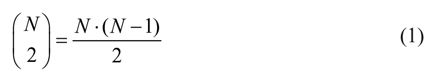
where N is the product of the number of cell levels.

Considering that properly powered decision-making experiments using HDDM can often require anywhere between 40 and 80 unique trials per decision type to achieve adequate power (Wiecki et al., 2013), factorial designs with several levels per factor substantially inflate the number of unique stimuli that need to be created, validated, and tested. This also extends the overall study duration and introduces participant fatigue concerns.

Step Three: Task Design

The third step is to create the decision options and design the decision trials. Note that the presentation format of the decision options needs to be simple since perceptual and cognitive processing of the stimulus will increase non-decision time and inflate non-decision time variability across trials, thereby dampening the estimation of DDM. We recommend using images or short-length text for decision options, both of which are easy to process and have good ecological validity (Supplemental Figure S3). To validate the decision option stimuli, we recommend asking participants to rate the attributes of the decision options to ensure that relevant attributes (e.g., arousal and valence) vary as designed in an orthogonal way. This can be achieved via stimulus pre-testing, as a manipulation check during the decision-making task, or (ideally) both.

After creating the decision option set, researchers can randomly draw two decision options from the decision option set to create a decision trial set. If multiple attributes are included, researchers should consider constructing the decision set in a factorial manner for all attributes as this facilitates analysis using linear modeling which estimates both the main effects for each attribute and the interaction between attributes.

Step Four: Task Programming

The fourth step is to design and implement the experiment. Here, researchers need to deliver the decision trials to participants in an experimental setting optimized for collecting choice and RT data. PsychoPy and PsychoJS are particularly suited for creating offline (PsychoPy) and online (PsychoJs) behavioral experiments like DDM. Advantages of each include (1) precise timing for measuring RT and presenting stimuli (Bridges et al., 2020); (2) hybrid methods comprising both an easy-to-use graphic user interface and access to the underlying code which gives high flexibility when creating the experimental logic; and (3) beginner-friendly demo libraries and good community support. We focus on PsychoJS, a java-script counterpart of the Python-based PsychoPy (Peirce et al., 2019). Implementing an experiment in either consists of three main components: initiating the experiment and defining stimuli, building experiment logistics in the experiment scheduler, and constructing routines.

To begin, researchers need to prepare the experiment stimuli, such as experiment instructions and visual/audio stimuli. The PsychoJS library provides a list of stimuli protocols, such as texts, shapes, images, soundtracks, or videos, and researchers need to specify the desired attributes for needed stimuli, such as content, color, position, or duration. In addition, researchers also need to define a list of necessary sensors to capture participants’ behavioral response data, which automatically record response data like participants’ keyboard presses or mouse movements.

Next, researchers need to build the logistics of the experiment, including the loops and transitions between sessions. Most experiments require multiple sessions such as instructions, training, induction, and measurement. These sessions need to be connected to define a triggered transition (e.g., keyboard press, timed transition). Each session, or block of sessions, can be reused by defining session loops. For instance, decision-making experiments demand repeated measures of response data in different decision tasks. The experimenter can specify a decision session and then repeat the sessions with varying stimuli via a loop.

Finally, researchers need to construct the routines for each experiment session. Depending on the purpose of the specific session, the timing and duration of the stimuli presentation and behavioral response sensors should be well specified. For instance, a typical cognitive experiment test session would normally start with a short presentation of a fixation cross stimulus to concentrate participants’ eye gaze on the center of the screen, followed by the experiment stimuli and keyboard pressing sensors.

Step Five: Power Analysis

The fifth step is to conduct a power analysis. This is determined both by the number of trials and the sample size. The number of trials per decision type is determined by the expected effect size and desired power level where power increases as the number of trials increases. For instance, 20 trials per decision type is the minimum required to accurately estimate DDM parameters, which gives power at 0.6 if the effect size is 0.3, and power at 0.8 if the effect size is 0.5 (Wiecki et al., 2013).

Sample size also impacts the accuracy of DDM estimation (Wiecki et al., 2013) and the capacity to detect a difference in parameters (Lerche et al., 2017). For instance, to reach the desired power at 0.6 to detect a significant within-subject main effect of decision type on a decision parameter, ~30 participants will be needed (Wiecki et al., 2013). When testing hypotheses using a regular linear model, researchers can estimate how many participants are needed by simulating RT datasets with varying participant sizes and trial sizes, then fitting a DDM with the simulated datasets and calculating the probability of detecting an effect. The HDDM package has a simulation tool that allows for such an analysis.

Step Six: Online Experimental Pipeline

Traditionally, behavioral experiments such as DDM were conducted in a university research laboratory. As a result, many behavioral experiments feature convenience samples of college students. By moving behavioral experiments online, it becomes possible to recruit a large number of subjects from the general population, thereby increasing a study’s generalizability. Accordingly, we focus on the steps necessary to build and implement an online DDM experimental paradigm. The design pipeline for an online behavioral experiment has three steps: building the experimental procedure (discussed above), hosting the experiment on a server, and recruiting participants (Sauter et al., 2020).

When hosting the experiment on a web server, researchers can choose their own private server, which offers maximum flexibility but requires high expertise to maintain, or a public server such as Pavlovia (https://pavlovia.org/), which consumes monetary credit for each completed participant. For smaller laboratories, we recommend using a public hosting server because it maintains the experimental code, allows source version control using GitLab, stores the collected data automatically, and reduces the effort required to maintain a private server.

The next step is recruiting participants. Researchers can recruit subjects as normal, via student sample platforms, such as SONA, or crowdsourcing platforms, such as M-Turk or Prolific Academic. If the target sample size is large and research resources allow, we recommend researchers consider data collection on crowdsourcing platforms due to faster data collection and more diverse participant samples. Regardless, the recruiting speed of online experiments with student samples is still much faster than offline laboratory experiments given that researchers are not constrained by the size of their laboratory.

Finally, researchers need to link each step in the pipeline with hyperlinks that transfer participants’ identification information through keys in the URL. An example study might consist of five components, SONA-Qualtrics-Pavlovia-Qualtrics-SONA (SQPQS), connected by a redirecting URL (Figure 2). The data are automatically stored as a comma-separated values (CSV) file on Pavlovia’s online server and can be downloaded for analysis.

Figure 2.

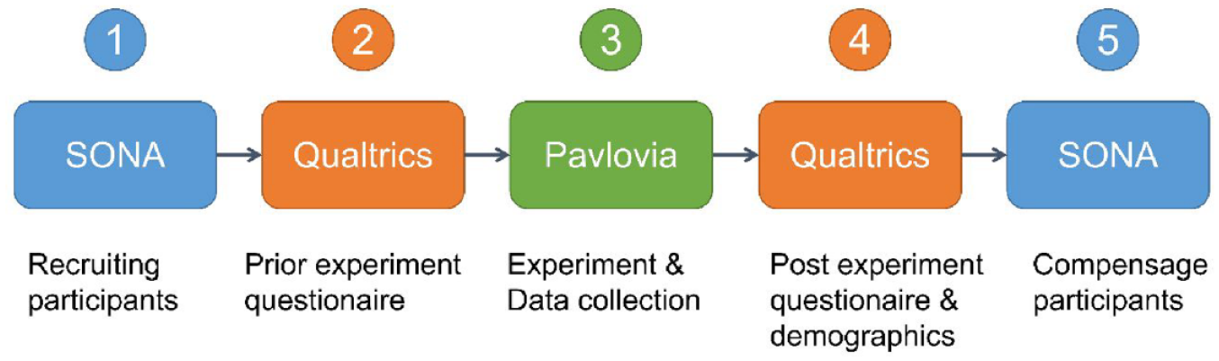
Online experimental pipeline for redirecting participants.

Step Seven: Model Fitting and Interpretation

The seventh step is to estimate the DDM. Multiple methods exist for fitting the DDM and estimating the parameters for hypothesis testing. There are three main approaches to estimate DDM, or generally any experimental behavioral model, which are quantile-based methods, maximum likelihood estimation (MLE), and a Bayesian approach. Quantile-based methods first summarize the collected RT data as quantiles (ranging from 0.1 to 0.9 quantiles), then use the extracted quantiles to compute goodness-of-fit measures for the model (i.e., chi-square value), and finally find the set of parameters values which maximize goodness-of-fit by minimizing the Chi-square measures (Ratcliff & McKoon, 2008). A quantile-based method is the simplest solution to estimate a DDM but usually performs the worst compared to other methods (Wiecki et al., 2013). Both MLE methods and Bayesian approaches use all RT data instead of subtracted quantile data summaries. Specifically, MLE methods compute the likelihood function of model parameters given observed RT data using the probability density function of RT distributions. Later, this likelihood function will be maximized, which produces the best-fit parameter values (Shinn et al., 2020). The Bayesian approach takes a similar step to calculate the likelihood function, but instead of maximizing the likelihood function, it uses the Bayes rule to compute the posterior probability of parameters using the likelihood function and the predefined prior distributions of parameters. One main difference between MLE and Bayesian approaches is that, without additional frequentist assumptions on the errors, MLE can only output point estimates of parameters (a singular value), but Bayesian approaches can generate the probability distributions of the parameters (Wiecki et al., 2013), which benefits researchers for hypothesis testing, data simulation, and making inferences, including inferences about null results (Kruschke, 2013).

Here we introduce a Bayesian approach using an HDDM (Wiecki et al., 2013), which has several advantages in that HDDM: (1) minimizes the required trial size to reach the same level of power; (2) offers a Bayesian approach that treats parameters as variables rather than a fixed number, thereby providing information about both the parameter estimates and the uncertainty of the estimates (i.e., the posterior probability distribution for parameter estimates); and (3) allows researchers to accept the null and falsify hypotheses by providing the explicit posterior distributions of parameters (Kruschke, 2013). In Supplemental Material Section 1, we give a detailed tutorial with code to estimate DDM using the HDDM package for interested readers.

In detail, HDDM (Supplemental Figure S4) specifies that the subject-level decision parameters (v, t, a, and z) are variables drawn from the group-level variables, and follow distributions governed by group-level parameters $(μ_{v}, σ_{v}, μ_{t}, σ_{t}, μ_{a}, σ_{a}, μ_{z}, σ_{z})$ . Thus, the estimates of the individual-level parameters are constrained by the group-level estimates and gradually update the group-level parameter estimates (Shiffrin et al., 2008). Then the posterior distribution of the group-level parameters is estimated using a Monte Carlo Markov chain method, which is a parameter sampling algorithm commonly used for Bayesian approaches (Gamerman & Lopes, 2014), with prior distributions of the group-level parameters and the likelihood of the observed RT data (positive/negative if choice is high/low value option) as a function of the subject-level decision parameters (Navarro & Fuss, 2009). In addition, due to the common existence of fast RT contaminates in the RT data,⁵ HDDM specifies a generative model for RT as a mixture model with a fixed probability (usually set to 0.05) of RTs coming from a uniform distribution of RT contaminants, and the remaining probability of RTs coming from the drift-diffusion process.

For each decision condition, such as the media decision type (i.e., attribute difference between the two media options), HDDM can separately estimate the specified group-level parameters (Supplemental Figure S4). Bayesian inference testing can be conducted using the posterior distributions of the group-level mean parameters $(μ_{v}, μ_{t}, μ_{a}, μ_{z})$ for each condition against the null value and constructing the highest density interval (HDI) to determine the credibility of parameter values relative to the null value (Kruschke, 2013). For instance, if a researcher hypothesizes a positive group-level parameter value (equivalent to a one-tailed test), specifies zero as the null value and 95% as a threshold, then they will interpret their result as “credible” if ≥95% of the HDI is >0.⁶

After DDM model fitting, the resulting posterior distributions will encode the effects of specified attributes on the decision parameters (i.e., mean or mode of the posterior distribution) as well as the uncertainty of the estimation (variance of the posterior distribution), which can be shown in Supplemental Figure S5. In our example, a positive effect for drift rate indicates a preference toward a high attribute value option, and a negative effect for drift rate indicates a preference toward a low attribute value option.

Concerns and Suggestions

Researchers might worry about the data quality of online behavioral experiments. Historically, laboratory-based research studies have allowed researchers to mitigate, or otherwise control for, numerous factors (e.g., heterogeneous computer hardware, participant distraction) that are difficult to deal with in online studies (Reips, 2002). Below, we provide some strategies for mitigating these concerns and solutions for diagnosing them in your data.

One of the major concerns is the accuracy of RT measures. Benchmarking research (Bridges et al., 2020) shows that PsychoJS has as good as (or better) timing accuracy (~3.5 ms) relative to most other experimental software (~10 ms), even after accounting for the substantial heterogeneity introduced by participant’s own computers.

Mitigating participant distraction requires considerable care. During any behavioral experiment, and especially during online behavioral experiments, participant fatigue and loss of interest can introduce speeding trends or autocorrelation in participants’ RT data across trials. This is an important concern since DDM usually assumes the observed data are iid (i.e., identical and independently distributed).

To address this concern, we first recommend piloting the experiment and tracking the time it takes participants to complete the study. Participants who complete online experiments often experience more distractions and pay less attention; therefore, short-duration online experiments are recommended (Sauter et al., 2020). It is not uncommon to see a long-tailed time-to-complete distribution with slow outliers. Despite this skew, in a recent study we conducted, the study time-to-complete distribution was centered about 50 minutes, which is roughly how long we expected the task to take (Supplemental Figure S6A). Time-to-complete data are a proxy for participant distraction; participants with exceptionally fast or slow time-to-complete metrics should be removed from further analysis. To help mitigate participant fatigue, distraction, and attrition, we recommend that experiments be kept as short as possible while also maintaining statistical power.

Another marker of distraction is a speeding trend across trials of the experiment. Distracted or fatigued participants might speed up their responses in an attempt to more quickly end the experiment. Speeding trends can be checked by correlating trial number and RT. As shown in Supplemental Figure S6B, a small (but negligible) speeding trend is observed in empirical data. Block designs can help mitigate this trend. We have found it particularly useful to give participants a short break between blocks, which has helped mitigate fatigue, speeding, and attrition. In fact, it appears that participant RT is contingent on the block design of the experiment. In a study we recently completed, RTs for each trial (Supplemental Figure S6C) and the autocorrelation of RTs across trials (Supplemental Figure S6D) show that the RT periodically decreases within each block, but RTs are brought back up by the break between blocks.

Finally, it is necessary to specify the exclusion criterion for failed participants and trials. We suggest including these criteria, along with data cleaning and inference procedures in a preregistration (Dienlin et al., 2021).

Conclusion

In this manuscript, we provided step-by-step guidance, along with sample code, for conducting and analyzing DDM studies collected via an online experiment. We provide some examples of ways to diagnose and mitigate potential concerns associated with online behavioral data collection. We hope that this helps other laboratories implement the DDM in their own research, mitigates the extent to which they must reinvent the wheel when developing these experimental paradigms in online contexts, and ultimately allows for the application of more complete explanations of human behavior (Huskey et al., 2020), including pressing challenges related to COVID-19 and beyond (see Supplemental Material Section 2).

Footnotes

Declaration of Conflicting Interests

The author(s) declared no potential conflicts of interest with respect to the research, authorship, and/or publication of this article.

Funding

The author(s) received no financial support for the research, authorship, and/or publication of this article.

ORCID iD

Xuanjun Gong

Supplemental Material

Supplemental material for this article is available online.

Notes

Author Biographies

Xuanjun Gong is a Ph.D. candidate at Department of Communication, UC, Davis. His research focus is on media selection, computational modeling, communication networks, and information diffusion. His research has been published in outlets such as Journal of Communication, Human Communication Research, Computational Communication Research, American Behavioral Scientist, and Journal of Medical Internet Research.

Richard Huskey (PhD, University of California Santa Barbara) is an Associate Professor in the Department of Communication and the Cognitive Science Program at the University of California Davis. Dr. Huskey is the principal investigator in the Cognitive Communication Science Lab, a researcher in the Computational Communication Research Lab, an affiliated faculty member at the Center for Mind and Brain, and an affiliated faculty member in the Designated Emphasis in Computational Social Science. He Chairs the International Communication Association Communication Science and Biology interest group, and is an Associate Editor at the Journal of Communication. He studies how motivation influences the attitudes people hold and the behaviors they adopt. He researches these questions using a variety of methodological techniques including: neuroimaging imaging (fMRI, EEG), computational modeling, and lab-based experimentation.

References

Adamowicz

Louviere

Swait

(1998). Introduction to attribute-based stated choice methods. https://ntrl.ntis.gov/NTRL/dashboard/searchResults/titleDetail/PB2003106817.xhtml

Agarwal

Hosanagar

Smith

M. D.

(2011). Location, location, location: An analysis of profitability of position in online advertising markets. Journal of Marketing Research, 48(6), 1057–1073. https://doi.org/10.1509/jmr.08.0468

Alós-Ferrer

Fehr

Netzer

(2021). Time will tell: Recovering preferences when choices are noisy. Journal of Political Economy, 129(6), 1828–1877. https://doi.org/10.1086/713732

Anwyl-Irvine

A. L.

Massonnié

Flitton

Kirkham

Evershed

J. K.

(2020). Gorilla in our midst: An online behavioral experiment builder. Behavior Research Methods, 52(1), 388–407. https://doi.org/10.3758/s13428-019-01237-x

Barbosa

Stein

Zorowitz

Niv

Summerfield

Soto-Faraco

Hyafil

(2022). A practical guide for studying human behavior in the lab. Behavior Research Methods, 55, 58–76. https://doi.org/10.3758/s13428-022-01793-9

Birnbaum

M. H.

(2004). Human research and data collection via the Internet. Annual Review of Psychology, 55(1), 803–832. https://doi.org/10.1146/annurev.psych.55.090902.141601

Bridges

Pitiot

MacAskill

M. R.

Peirce

J. W.

(2020). The timing mega-study: Comparing a range of experiment generators, both lab-based and online. PeerJ, 8, e9414. https://doi.org/10.7717/peerj.9414

Bode

Sewell

D. K.

Lilburn

Forte

J. D.

Smith

P. L.

Stahl

(2012). Predicting perceptual decision biases from early brain activity. The Journal of Neuroscience, 32(36), 12488–12498. https://doi.org/10.1523/JNEUROSCI.1708-12.2012

Clifford

Jerit

(2014). Is there a cost to convenience? An experimental comparison of data quality in laboratory and online studies. Journal of Experimental Political Science, 1(2), 120–131. https://doi.org/10.1017/xps.2014.5

10.

Clithero

J. A.

(2018). Improving out-of-sample predictions using response times and a model of the decision process. Journal of Economic Behavior & Organization, 148, 344–375. https://doi.org/10.1016/j.jebo.2018.02.007

11.

Craswell

Zoeter

Taylor

Ramsey

(2008). An experimental comparison of click position-bias models. In Proceedings of the 2008 international conference on web search and data mining, Palo Alto, CA, USA, 11–12 February 2008 (pp. 87–94). ACM. https://doi.org/10.1016/j.jebo.2018.02.007

12.

Dayan

Daw

N. D.

(2008). Decision theory, reinforcement learning, and the brain. Cognitive, Affective, & Behavioral Neuroscience, 8(4), 429–453. https://doi.org/10.3758/CABN.8.4.429

13.

Dienlin

Johannes

Bowman

N. D.

Masur

P. K.

Engesser

Kumpel

A. S.

Lukito

Bier

L. M.

Zhang

Johnson

B. K.

Huskey

Schneider

F. M.

Breuer

Parry

D. A.

Vermeulen

Fisher

J. T.

Banks

Weber

Ellis

D. A.

, . . .Vreese

C. D.

(2021). An agenda for open science in communication. Journal of Communication, 71(1), 1–26. https://doi.org/10.1093/joc/jqz052

14.

Gamerman

Lopes

H. F.

(2014). Markov chain Monte Carlo: Stochastic simulation for Bayesian inference (2nd ed.). Chapman and Hall/CRC.

15.

Hainmueller

Hangartner

Yamamoto

(2015). Validating vignette and conjoint survey experiments against real-world behavior. Proceedings of the National Academy of Sciences, 112(8), 2395–2400. https://doi.org/10.1073/pnas.1416587112

16.

Hartmann

(2009). Media choice: A theoretical and empirical overview. Routledge.

17.

Huskey

Bue

A. C.

Eden

Grall

Meshi

Prena

Schmälzle

Scholz

Turner

B. O.

Wilcox

(2020). Marr’s tri-level framework integrates biological explanation across communication subfields. Journal of Communication, 70(3), 356–378. https://doi.org/10.1093/joc/jqaa007

18.

Klauer

K. C.

Voss

Schmitz

Teige-Mocigemba

(2007). Process components of the implicit association test: A diffusion-model analysis. Journal of Personality and Social Psychology, 93(3), 353–368. https://doi.org/10.1037/0022-3514.93.3.353

19.

Knobloch-Westerwick

(2014). Choice and preference in media use: Advances in selective exposure theory and research. Routledge.

20.

Kowalczyk

A. W.

Grange

J. A.

(2020). The effect of episodic retrieval on inhibition in task switching: A diffusion model analysis. Psychological Research, 84(7), 1965–1999. https://doi.org/10.1007/s00426-019-01206-1

21.

Krajbich

Camerer

Rangel

(2012). The attentional drift-diffusion model extends to simple purchasing decisions. Frontiers in Psychology, 3, 1–18. https://doi.org/10.3389/fpsyg.2012.00193

22.

Kruschke

J. K.

(2013). Bayesian estimation supersedes the t test. Journal of Experimental Psychology: General, 142(2), 573–603. https://doi.org/10.1037/a0029146

23.

Lerche

Voss

Nagler

(2017). How many trials are required for parameter estimation in diffusion modeling? A comparison of different optimization criteria. Behavior Research Methods, 49(2), 513–537. https://doi.org/10.3758/s13428-016-0740-2

24.

Lerche

Voss

(2016). Model complexity in diffusion modeling: Benefits of making the model more parsimonious. Frontiers in Psychology, 7, 1324. https://doi.org/10.3389/fpsyg.2016.01324

25.

Lin

Pennycook

Rand

D. G.

(2023). Thinking more or thinking differently? Using drift-diffusion modeling to illuminate why accuracy prompts decrease misinformation sharing. Cognition, 230, 105312. https://doi.org/10.1016/j.cognition.2022.105312

26.

Milosavljevic

Malmaud

Huth

Koch

Rangel

(2010). The drift diffusion model can account for the accuracy and reaction time of value-based choices under high and low time pressure. Judgment and Decision Making, 5(6), 437–449. https://doi.org/10.1017/S1930297500001285

27.

Navarro

D. J.

Fuss

I. G.

(2009). Fast and accurate calculations for first-passage times in Wiener diffusion models. Journal of Mathematical Psychology, 53(4), 222–230. https://doi.org/10.1016/j.jmp.2009.02.003

28.

Parry

D. A.

Davidson

B. I.

Sewall

C. J. R.

Fisher

J. T.

Mieczkowski

Quintana

D. S.

(2021). A systematic review and meta-analysis of discrepancies between logged and self-reported digital media use. Nature Human Behaviour, 5(11), 1535–1547. https://doi.org/10.1038/s41562-021-01117-5

29.

Peirce

Gray

J. R.

Simpson

MacAskill

Höchenberger

Sogo

Kastman

Lindeløv

J. K.

(2019). PsychoPy2: Experiments in behavior made easy. Behavior Research Methods, 51(1), 195–203. https://doi.org/10.3758/s13428-018-01193-y

30.

Ratcliff

(1993). Methods for dealing with reaction time outliers. Psychological Bulletin, 114(3), 510–532. https://doi.org/10.1037/0033-2909.114.3.510

31.

Ratcliff

Frank

M. J.

(2012). Reinforcement-based decision making in corticostriatal circuits: Mutual constraints by neurocomputational and diffusion models. Neural Computation, 24(5), 1186–1229. https://doi.org/10.1162/NECO_a_00270

32.

Ratcliff

Hendrickson

A. T.

(2021). Do data from mechanical Turk subjects replicate accuracy, response time, and diffusion modeling results? Behavior Research Methods, 53(6), 2302–2325. https://doi.org/10.3758/s13428-021-01573-x

33.

Ratcliff

McKoon

(2008). The diffusion decision model: Theory and data for two-choice decision tasks. Neural Computation, 20(4), 873–922. https://doi.org/10.1162/neco.2008.12-06-420

34.

Ratcliff

Philiastides

M. G.

Sajda

(2009). Quality of evidence for perceptual decision making is indexed by trial-to-trial variability of the EEG. Proceedings of the National Academy of Sciences, 106(16), 6539–6544. https://doi.org/10.1073/pnas.0812589106

35.

Ratcliff

Smith

P. L.

Brown

S. D.

McKoon

(2016). Diffusion decision model: Current issues and history. Trends in Cognitive Sciences, 20(4), 260–281. https://doi.org/10.1016/j.tics.2016.01.007

36.

Reips

U. D.

(2002). Standards for internet-based experimenting. Experimental Psychology, 49(4), 243. https://doi.org/10.1026/1618-3169.49.4.243

37.

Sauter

Draschkow

Mack

(2020). Building, hosting and recruiting: A brief introduction to running behavioral experiments online. Brain Sciences, 10(4), 251. https://doi.org/10.3390/brainsci10040251

38.

Schoemann

O’Hora

Dale

Scherbaum

(2021). Using mouse cursor tracking to investigate online cognition: Preserving methodological ingenuity while moving toward reproducible science. Psychonomic Bulletin & Review, 28(3), 766–787. https://doi.org/10.3758/s13423-020-01851-3

39.

Shiffrin

R. M.

Lee

M. D.

Kim

Wagenmakers

E.-J.

(2008). A survey of model evaluation approaches with a tutorial on hierarchical Bayesian methods. Cognitive Science, 32(8), 1248–1284. https://doi.org/10.1080/03640210802414826

40.

Shinn

Lam

N. H.

Murray

J. D.

(2020). A flexible framework for simulating and fitting generalized drift-diffusion models. ELife, 9, e56938. https://doi.org/10.7554/eLife.56938

41.

Smith

P. L.

Ratcliff

(2004). Psychology and neurobiology of simple decisions. Trends in Neurosciences, 27(3), 161–168. https://doi.org/10.1016/j.tins.2004.01.006

42.

Stafford

Pirrone

Croucher

Krystalli

(2020). Quantifying the benefits of using decision models with response time and accuracy data. Behavior Research Methods, 52, 2142–2155. https://doi.org/10.3758/s13428-020-01372-w

43.

Wilcox

Huskey

DeAndrea

D. C.

(2021). Attitude-consistent health messages about electronic cigarettes increase processing time. Journal of Media Psychology: Theories, Methods, and Applications, 34(4), 216–229. https://doi.org/10.1027/1864-1105/a000312

44.

Wilson

R. C.

Collins

A. G.

(2019). Ten simple rules for the computational modeling of behavioral data. Elife, 8, e49547. https://doi.org/10.7554/eLife.49547

45.

Wiecki

T. V.

Sofer

Frank

M. J.

(2013). HDDM: Hierarchical Bayesian estimation of the drift-diffusion model in python. Frontiers in Neuroinformatics, 7, 14. https://doi.org/10.3389/fninf.2013.00014

46.

Zillmann

(1988). Mood management through communication choices. American Behavioral Scientist, 31(3), 327–340. https://doi.org/10.1177/000276488031003005

Supplementary Material

Please find the following supplemental material available below.

For Open Access articles published under a Creative Commons License, all supplemental material carries the same license as the article it is associated with.

For non-Open Access articles published, all supplemental material carries a non-exclusive license, and permission requests for re-use of supplemental material or any part of supplemental material shall be sent directly to the copyright owner as specified in the copyright notice associated with the article.

0.00 MB

1.34 MB

Moving Behavioral Experimentation Online: A Tutorial and Some Recommendations for Drift Diffusion Modeling

Abstract

Keywords

Behavioral Modeling

The Drift Diffusion Model

Challenges of Moving DDM Online

An End-to-End Pipeline for Conducting and Analyzing an Online DDM Experiment

Step One: Hypothesis Formation

Step Two: Attribute Selection

Step Three: Task Design

Step Four: Task Programming

Step Five: Power Analysis

Step Six: Online Experimental Pipeline

Step Seven: Model Fitting and Interpretation

Concerns and Suggestions

Conclusion

Footnotes

Declaration of Conflicting Interests

Funding

ORCID iD

Supplemental Material

Notes

Author Biographies

References

Supplementary Material