Sage Journals: Discover world-class research

Abstract

We revisit a key question about poverty that was a repeated subject of investigation for Rebecca Blank, estimating the effects of the business cycle on pre–tax-and-transfer and post–tax-and-transfer poverty. Using an anchored household-level version of the Supplemental Poverty Measure’s thresholds and resources, we show that poverty is countercyclical, rising in recessions and falling in expansions. We also find that the social safety net provides protection against cyclicality: Post–tax-and-transfer poverty is less cyclical than is pre–tax-and-transfer poverty. The largest cyclicality occurs among children and Black and Hispanic persons, and lower cyclicality is evident among white and elderly persons. The safety net leads to the largest reductions in cyclicality for the elderly and the smallest effects for nonelderly households without children. Finally, we find an inverted U shape with cyclicality low and rising below 75 percent of poverty and declining above.

Keywords

macroeconomy poverty cyclicality supplemental poverty

In this article, we revisit a question that Rebecca “Becky” Blank took up with coauthors Alan Blinder and David Card (Blank and Blinder 1986; Blank and Card 1993): What is the impact of macroeconomic conditions on poverty? These were the first works to examine the cyclicality of economic well-being across the income distribution, with a particular focus on the lower end of the income distribution. Their work examined how these impacts varied with alternative measures of the economic cycle, how cyclicality varied across demographic groups, and what role the safety net played in buffering these shocks. As with many topics, Becky Blank made significant contributions and opened up new inquiries. In this case, her work expanded the macro lens on impacts of recessions to distributional impacts with a focus on possible roles for policy.

We begin by summarizing these pioneering studies and the literature that followed. The work has evolved over time as poverty measurement has advanced from use of the Official Poverty Measure (OPM) to the Supplemental Poverty Measure (SPM). Becky’s work and the work that followed show that the cyclicality of poverty is not a stable parameter but can and does change with structural changes in the labor market and the social safety net.

We then provide updates and new estimates for the cyclicality of poverty using data through 2019 (pre-COVID) as well as through 2022. We use data from the Current Population Survey (CPS) Annual Social and Economic Supplement (ASEC) files and construct two main measures of poverty—pre–tax-and-transfer and post–tax-and-transfer poverty—to show how excluding or including government taxes and transfers from household resources affects measured poverty rates and their cyclicality. For both poverty rates, we compare household-level resources to an anchored household-level version of the SPM’s thresholds. Using state-by-year data, we estimate the impact of two measures of local labor markets—state unemployment and real median income—on poverty. Following Becky’s work, we examine how this varies by demographic group and at different points in the income-to-poverty distribution.

We find that poverty is countercyclical, rising in recessions and falling in expansions. We also show that the social safety net protects against volatility in the rises and falls of the cycles: Post–tax-and-transfer poverty is less cyclical than is pre–tax-and-transfer poverty. The effects of business cycles on pre–tax-and-transfer poverty vary significantly across demographic groups, with the largest cyclicality for children and Black and Hispanic persons and lower cyclicality for white and elderly persons. While the safety net leads to reductions in cyclicality for almost all groups, there is large variation in its impact, with the largest reductions in cyclicality for the elderly and the smallest reductions for Hispanics and nonelderly households without children. Finally, we study how our results vary across the income to poverty distribution. We find an inverted U shape with cyclicality low at 25 percent of poverty, rising until 75 percent of poverty, and declining at higher thresholds of poverty. Overall, our results suggest that further safety net spending aimed at children, minorities, or individuals with household incomes between 25 and 150 percent of poverty thresholds might be most effective at reducing the cyclicality of economic well-being.

Prior Work on Macroeconomics and Poverty

Becky’s work in this area began with a straightforward question: How do poverty and the income distribution respond to the business cycle and economic growth? Blank and Blinder (1986) use time series data and estimate the impact of inflation and the unemployment rate on official poverty rates (1959–1983) and income shares (1948–1983). They find that a 1 percentage point increase in the national unemployment rate leads to a 0.69 percentage point increase in the national poverty rate. They also explore differences by age, by race, and by lower- versus higher-wage groups. In describing these results, they state, “Our analysis confirms this view [rising tide raises all boats] and indicates that the smallest boats get raised the most (relatively). Conversely, however, they also fall the most when the tide ebbs—a point to keep in mind when the unemployed are drafted to fight the war on inflation” (Blank and Blinder 1986, 207).

Blank and Card (1993) also address this question, but they point out the importance of using panel data. In particular, they construct data at the Census region-by-year level to leverage across-area variation in economic growth and unemployment. Using data for 1967–1991, they examine whether there had been changes in the cyclicality of poverty in the 1980s, a period during which there were reductions in unemployment and little decline in poverty. They find that a 1 percentage point increase in the unemployment rate led to a 0.2 percentage point increase in poverty—confirming that the relationship between the macroeconomy and poverty did in fact weaken. They go on to explore impacts by subgroup and decompose the changes into explained versus unexplained components.

In this work and in other related papers (e.g., Blank 1993; Blank and Ruggles 1992, 2000), a core question was the role of the safety net in softening the effects of economic downturns on poverty. In Blank and Card (1993), the authors show that government transfers—their analysis captures cash transfers, including unemployment insurance, disability, and cash welfare—reduce poverty rates but conclude that “detailed data on transfer programs by region are clearly needed to provide further evidence [on the role of transfers]” (322).

This work has had a significant impact on our own research, in which we have continued to explore the questions raised by Becky and her coauthors. In particular, we have examined how cyclicality has varied over time, how it varies across groups, and what role the social safety net plays in buffering the shocks of labor market fluctuations.

Blank and Blinder (1986) and Blank and Card (1993) relied on the OPM, which was created in the 1960s and, roughly speaking, compares a family’s pretax cash income to poverty thresholds, based on updating estimates of the level of income needed in the 1960s by the Consumer Price Index.¹ As Johnson et al. (this volume) describe in another contribution to this volume, Becky helped produce the 1995 National Academies Report pointing out various weaknesses in the OPM and calling for reforms to the poverty measure (National Research Council 1995). Further, while serving in government and other policy positions, Becky championed the development of a new, improved poverty measure to address these weaknesses (e.g., Blank 2008a, 2008b; Blank and Greenberg 2008). This led to the creation of the SPM (Short 2011), which the Census Bureau first released in 2011 and now issues, along with the OPM, each fall. The OPM uses cash income, calculated before taxes, to measure resources. The SPM incorporates taxes (including tax credits) and in-kind transfers, such as Supplemental Nutrition Assistance Program (SNAP, known earlier as Food Stamps); housing vouchers; Special Supplemental Nutrition Program for Women, Infants, and Children (WIC); and school meals. Tax credits and in-kind transfers have been an increasingly important component of the U.S. safety net over time, particularly since the mid-1990s. Additionally, the OPM threshold is fixed across the mainland U.S. and does not account for differences in the cost of living across places, while the SPM threshold varies by geographic areas finer than state.

Using a broader measure of resources, based on the SPM’s resource measure, Bitler and Hoynes (2016) examine how the cyclicality of poverty has changed over time. They find that after welfare reform and the rise of the Earned Income Tax Credit (EITC) in the 1990s, the cyclicality of poverty increased. They go on to analyze the cyclicality of various components of the social safety net and find that post–welfare reform, cash welfare (Aid to Families with Dependent Children/Temporary Assistance for Needy Families [AFDC/TANF]) entirely loses its countercyclicality. Further, Bitler, Hoynes, and Kuka (2017b) show that the EITC is less likely to provide protection in recessions than in good economic times. Reflecting the tax credit’s work requirement, they find that the EITC is even weakly procyclical for single-parent families (although not statistically significantly so). However, despite shifts toward an in-work safety net in the 1990s, Bitler, Hoynes, and Kuka (2017a) show that, on net, the tax and transfer system—writ large—still reduces exposure to business cycles for families with children. When separately considering means-tested transfers (e.g., SNAP, cash welfare), social insurance (e.g., Social Security, disability, unemployment insurance), and the tax system (e.g., EITC), we find that for children, means-tested transfers and tax credits were the most important factors in driving this reduction in cyclicality.

New Evidence on Macroeconomics and Poverty: Data, Poverty Measures, and Methods

Data

We use the CPS ASEC. Each year, primarily in March, the ASEC augments the usual core CPS questions on labor markets and demographics to measure individuals’ incomes and program participation over the previous calendar year. The ASEC asks adults aged 15 and older directly about the presence and amount of private income from a host of pretax cash sources, including wage and salary income, farm income, self-employment income, private disability, and pension/other retirement benefits. It also includes a host of social-insurance and means-tested safety net cash benefits, including Old Age and Disability Insurance Social Security Benefits, Supplemental Security Income, unemployment insurance, workers’ compensation, veteran’s benefits, and cash welfare (including TANF as well as state and local general assistance). Finally, the ASEC asks about a range of in-kind benefits and, for some, asks about benefit amounts. These include SNAP, the National School Lunch Program (NSLP), the Low-Income Heating Assistance Program (LIHEAP), and public housing assistance. The Census Bureau also imputes whether a household receives aid from other safety net programs and the amount of aid that household receives. This includes the WIC program, where receipt and the dollar value of benefits are imputed, as well as housing subsidies, LIHEAP, and the NSLP, where only the dollar values of benefits are imputed. Finally, the Census Bureau models the impact of federal and state tax systems, including tax credits such as the EITC and Child Tax Credit (CTC), and tax payments. We combine these (as discussed below) to get a pre–tax-and-transfer and post–tax-and-transfer concept of resources.

We focus on CPS ASEC survey years 2001–2020, covering calendar years from 2000 to 2019, but also explore robustness by looking at the period from 2000 to 2022 (including the enormous shock of COVID-19 and ensuing response). In order to investigate poverty and the business cycle for all persons and demographic subgroups of persons, we calculate person-level poverty rates and aggregate these to average rates at the level of state by year by demographic group. These include groupings by age (0–17, 18–64, 65 and above), by family type (household head 65 and older, household head under 65 with children in the household, household head under 65 with no children in the household), and by race/ethnicity (non-Hispanic white [“white” from now on], non-Hispanic Black [“Black” from now on], Hispanic, and, reported in some tables, everyone else who is non-Hispanic [denoted as “Other” from now on]).

Poverty measures

In this article, we use measures of pre–tax-and-transfer and post–tax-and-transfer income (similar to what we used in Bitler, Hoynes, and Kuka 2017a) and an anchored version of the 2021 SPM thresholds (from Creamer et al. 2022) to calculate household-level poverty measures. We begin by summing up the income or resources (of whatever form) for every person in the same dwelling and then compare this to the relevant threshold for a unit of the size of the number of persons in the household.² Each person in the household is assigned the household poverty measure.

To use the standard SPM back to 2000 would require a number of measures of income and expenditures beyond what is available with the Census Bureau’s SPM releases, which only go back to 2009. There are several approaches to constructing a consistent series that have been created by the Center on Poverty and Social Policy at Columbia and generously shared (e.g., Wimer et al. 2016). To maintain comparability over time, we choose a version of the anchored SPM, which takes SPM thresholds from a specific year and adjusts them forward and backward with a measure of Consumer Price Index (CPI) inflation. We make use of data made available by the Columbia colleagues (Wimer et al. 2023).

These anchored SPM measures start with SPM thresholds from the Bureau of Labor Statistics (BLS) provided for a standardized household size and separately for renters, owners with mortgages, and owners without mortgages across geographic areas. These thresholds are then adjusted with an equivalence scale for the number of persons by age in the unit, and then we adjust them backward in time using a measure of inflation (we use the historical research series CPI for all Urban Consumers [CPI-U-RS]). The final step is to adjust these with a multiplicative factor for geographic differences in the cost of housing (here set at the value in the anchor year, 2021).

We use these thresholds to construct two measures of SPM poverty: pre–tax-and-transfer SPM poverty and post–tax-and-transfer SPM poverty. Both use the same anchored poverty thresholds, and they differ only in their definition of resources. Our post–tax-and-transfer resource measure uses the SPM concept of resources³ with one exception. Our post–tax-and-transfer measure of resources does not subtract out medical out-of-pocket spending, child support paid, and other work and child care spending (which we do not observe back to 2000 in the CPS ASEC). Following Bitler, Hoynes, and Kuka (2017a), our pre–tax-and-transfer resource measure includes all private income in the household. Our third poverty measure, which we use in some models, is the OPM (cash pretax income inclusive of cash transfers compared to OPM thresholds).

We show these pre– and post–tax-and-transfer SPM measures in Figures 1 and 2. Figure 1 plots the official poverty rate (black solid lines with circles) and the post–tax-and-transfer SPM poverty rate (blue long dashed line with circles) for all persons as well as the national unemployment rate (red short dashed line with diamonds) from 2000 to 2022. It is clear from the graph that the OPM moves more with fluctuations in unemployment compared to the SPM. The OPM and SPM measures were similar in 2000 but diverged more during the period around the Great Recession and the COVID-19 crisis, when the economy was under great duress and the tax and transfer system would be expected to be strong. Figure 2 plots the pre– and post–tax-and-transfer SPM rates over the same 2000–2022 period, showing the discrepancy between these measures is largest during COVID-19 and, to a lesser extent, during the Great Recession.

Figure 1

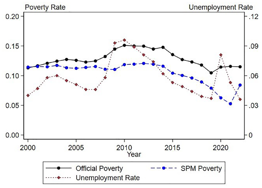
Official Poverty and Anchored Supplemental Poverty Measure for All Persons Along with U.S. Unemployment Rate, 2000–2022

Figure 2

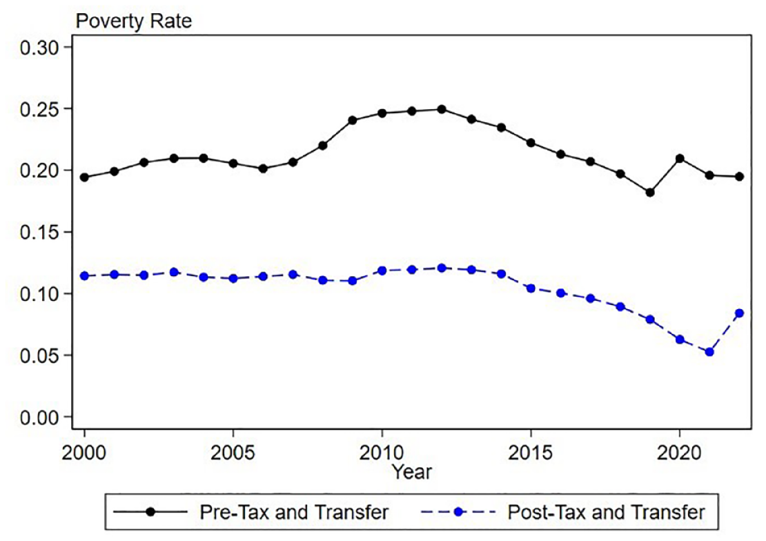
Supplemental Poverty Measure, Pre– and Post–Tax-and-Transfers, All Persons, 2000–2022

Methods

We model the effects of the business cycle on both pre–tax-and-transfer and post–tax-and-transfer poverty. Following the approach taken in Becky’s studies, we explore two measures of the business cycle. Our main measure is the annual unemployment rate (from the BLS), and we also consider real median household income published by the Census Bureau, based on the CPS ASEC.

We start by following the approach in Blank and Blinder (1986) and estimate time series regressions of the following form:

y_{t} = α + β * L M_{t} + ε_{t},

(1)

where y_t is the national (pre– or post–tax-and-transfer) poverty rate for all persons in year t, and LM_t is the national labor market measure (e.g., unemployment or real median income). The parameter of interest, β, captures the impact of the labor market on poverty. The regressions are weighted by the sum of the CPS weights for the persons in year t.

Then we turn to panel data and estimate panel data regressions of the following form:

y_{s t} = α + β * L M_{s t} + η_{s} + λ_{t} + ε_{s t},

(2)

where the data is at the state-by-year level. Here, y_st is the (pre– or post–tax-and-transfer) poverty rate for all persons in state s in year t. Analogously, LM_st, the unemployment rate in state s in year t (measured in percentage points so a one-unit increase is a 1 percentage point increase), is our measure of the local economy in state s in year t. We also control for fixed effects for state (η_s) and year (λ_t). As originally discussed in Blank and Card (1993), the advantage of using this state-by-year data is that we identify the impacts of the labor market on poverty using variation across states in the magnitude of expansions and recessions while holding constant national trends (which may capture factors other than business cycles). The regressions are weighted by the sum of the CPS weights for the persons in each state-year cell, and the panel data variance-covariance matrices allow for arbitrary correlations within state.

Following Blank and Blinder (1986) and Blank and Card (1993), we also explore differences in the effect of the business cycle on individual poverty across different demographic groups.⁴ We present results for the following 10 groups: all persons; groups by the age of the person (children aged 0–17, adults aged 18–64, and older adults aged 65 and older); groups by the race/ethnicity of the person (white non-Hispanic, Black non-Hispanic, or Hispanic); groups by household type (elderly household head, nonelderly household head with at least one child aged 17 or younger in the household, and nonelderly household head and no child in the household).⁵ We focus on the period from 2000 to 2019 but also show the effects in many cases, including the COVID-19 period through 2022, which included both a very severe economic shock and massive fiscal responses from the federal government.

Results: New Evidence on Macroeconomics and Poverty

Table 1 reports the pre–tax-and-transfer (column 1) and post–tax-and-transfer (column 2) SPM poverty measures, for all persons, and for each of our demographic groups (by person’s age, person’s race/ethnicity, and household type), averaged over the years 2000–2019. The third column shows the percent change in the poverty rate from adding net income from the tax and transfer system to the pre–tax-and-transfer resource measure. This table reveals familiar patterns. Using pre–tax-and-transfer income, we see that the elderly (65 and older) face the highest poverty rates and then children; prime-age adults face the lowest rates. This pattern changes once we consider the post–tax-and-transfer income measure. Now children face the highest rates, then prime-age adults, and then the elderly. (Note here the difference with the Census SPM, which subtracts out from resources medical out-of-pocket spending, which is very large for the elderly.) Both the pretax and posttax SPM show higher rates for Black and Hispanic persons than for white and other race persons. Turning to the final column, the tax and transfer system reduces poverty rates for all groups. However, the largest reductions are for those 65 and over (a 77 percent reduction), followed by white persons (61 percent reduction), with lower rates for children (37 percent reduction), Black persons (42 percent reduction), and Hispanic persons (33 percent reduction).

Table 1

Who Is Poor in the United States (Supplemental Poverty Threshold)

	Share of Persons Poor, 2000–2019
	Pre–Tax-and-Transfer Income (column 1)	Post–Tax-and-Transfer Income (column 2)	Percent Change
All persons	0.217	0.110	−49.3%
Age of person
Less than 18	0.223	0.137	−38.6%
18–64	0.160	0.102	−36.3%
65+	0.464	0.098	−78.9%
Race/ethnicity of person
White non-Hispanic	0.172	0.067	−61.0%
Black non-Hispanic	0.343	0.198	−42.3%
Hispanic	0.306	0.204	−33.3%
Other race	0.200	0.125	−37.5%
Household type
Elderly head	0.451	0.102	−77.4%
Nonelderly head, with children	0.193	0.122	−36.8%
Nonelderly head, without children	0.144	0.095	−34.0%

SOURCE: Authors’ calculations using 2001–2020 ASEC (2000–2019 calendar years).

NOTE: Resource measure is pre–tax-and-transfer resources (column 1) and post–tax-and-transfer resources (column 2), and the economic resource unit is the household. The poverty thresholds are the 2021 SPM thresholds, anchored with geographic adjustment; the CPI-U-RS is used to adjust back in time. All poverty rates are at the person level.

Next, we turn to regressions, looking at the systematic relationship of poverty to the business cycle across our groups. Table 2 starts by replicating the time series work of Blank and Blinder (1986), looking at the effects of the national business cycle on the OPM. Blank and Blinder used data for 1959–1983; we look at 2000–2019. Column 1 shows the effect of the unemployment rate on official poverty, finding a 1 percentage point increase in the unemployment rate leads to a 0.66 percentage point increase in official poverty, falling closer to the Blank and Blinder estimate (0.69) from the period before the 1980s than to that of Blank and Card (1993) (0.20). Column shows the corresponding relationship, using real median state income to measure the business cycle, finding that a $1,000 increase in real median income leads to a 0.38 percentage point reduction in official poverty. Columns 3 and 4 show the results of the analogous state-year level panels. Both columns show that identifying the cyclical relationship using panel data and deviations from state averages and net of national trends leads to a reduction in estimated cyclicality. Column 3 shows that a 1 percentage point increase in the unemployment rate leads to a 0.53 percentage point increase in the OPM, while a $1,000 increase in real median income leads to a 0.21 percentage point reduction in official poverty. Since using the state unemployment rate or real median state income as a measure of the business cycle yields similar qualitative results on the cyclicality of poverty, we focus on the unemployment rate for the remainder of this article.

Table 2

Cyclicality of Poverty Using Official Poverty Measure, All Persons, 2000–2019

	National Time Series		State-Year
	OPM	OPM	OPM	OPM
Unemployment rate	0.663*** (0.075)		0.528*** (0.059)
Real income (10,000s)		−0.038*** (0.004)		−0.021*** (0.002)
Mean Y	0.130	0.130	0.130	0.130
Mean state cycle variable	0.059	6.446	0.059	6.535
N	20	20	1,020	1,020

SOURCE: Authors’ calculations using 2001–2020 ASEC (2000–2019 calendar years).

NOTE: Columns 1 and 2 use data by year and include year fixed effects. Columns 3 and 4 use state-by-year data and include fixed effects for state and year. Poverty is measured using the official poverty measure. State-by-year regressions weighted by population weights. Variance-covariances allowed to vary arbitrarily within state.

***

refers to significance at the .01 level.

Given the documented weaknesses of the OPM, one could worry these estimates are missing the potentially important protective effects of in-kind transfers and taxes, not measured in the cash-oriented, pretax OPM. Next, we turn to estimates that use the SPM. We start with Table 3, where column 1 presents results for the pre–tax-and-transfer SPM and column 2 presents results for the post–tax-and-transfer SPM. Both use state-by-year data and, as in equation (2), control for state and year fixed effects. The results show that from 2000 to 2019, a 1 percentage point increase in the unemployment rate leads to a 0.86 percentage point increase in pre–tax-and-transfer SPM poverty. Post–tax-and-transfer SPM poverty is less cyclical, where a 1 percentage point increase in the unemployment rate leads to a 0.70 percentage point increase in poverty. This illustrates the capacity of the safety net, social insurance, and tax systems to buffer the effects of business cycles.

Table 3

Cyclicality of Poverty Using Supplemental Poverty Threshold Pre– and Post–Tax-and-Transfer, All Persons, 2000–2019 and 2000–2022

	2000–2019		2000–2022
	SPMPre-TT	SPMPost-TT	SPMPre-TT	SPMPost-TT
Unemployment rate	0.858*** (0.093)	0.701*** (0.132)	0.652*** (0.097)	0.452*** (0.129)
Mean Y	0.217	0.110	0.215	0.104
Mean state cycle variable	0.059	0.059	0.059	0.059
N	1,020	1,020	1,173	1,173

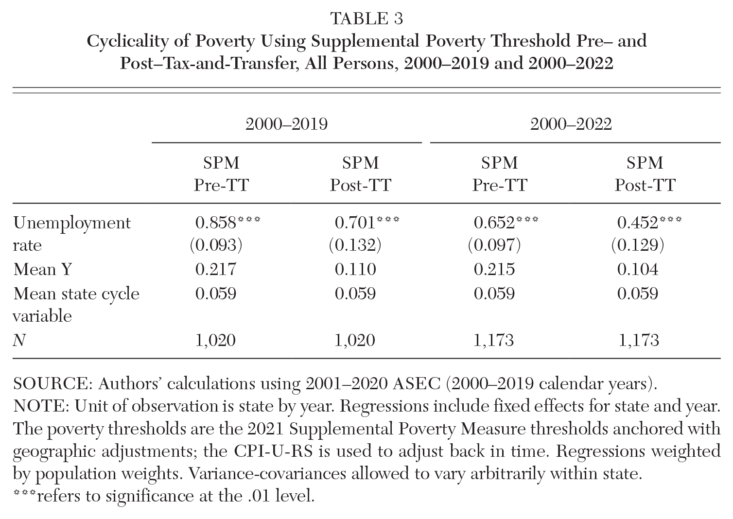
SOURCE: Authors’ calculations using 2001–2020 ASEC (2000–2019 calendar years).

NOTE: Unit of observation is state by year. Regressions include fixed effects for state and year. The poverty thresholds are the 2021 Supplemental Poverty Measure thresholds anchored with geographic adjustments; the CPI-U-RS is used to adjust back in time. Regressions weighted by population weights. Variance-covariances allowed to vary arbitrarily within state.

***

refers to significance at the .01 level.

The remainder of the table shows the estimates using data extended through the COVID-19 period (through 2022). The estimates for cyclicality of poverty are smaller in magnitude when we add the additional three years of the COVID-19 period (although not significantly so). We find that a 1 percentage point increase in unemployment leads to a 0.65 percentage point increase in pre–tax-and-transfer SPM poverty (compared to 0.86 for 2000–2019). A 1 percentage point increase in unemployment leads to a 0.45 percentage point increase in post–tax-and-transfer SPM poverty (compared to 0.70 for 2000–2019). This is consistent with the much more robust fiscal response to the pandemic (e.g., including expansions in unemployment insurance, SNAP, stimulus checks, the EITC, and the CTC) compared to the Great Recession (Bitler, Hoynes, and Schanzenbach 2020, 2023).

Table 4 presents our post–tax-and-transfer SPM poverty measure’s responsiveness to the unemployment rate, across subgroups of persons. Here, in addition to the point estimates, we also present percentage impacts or the ratio of the coefficient on the unemployment rate to the mean of the dependent variable (since the unemployment rates are measured at the state-by-year level and are nearly the same across all the samples). We see that persons in households with children (with nonelderly household heads) and Hispanic persons have poverty that is the most responsive—in terms of percentage impacts—to the business cycle. Reflecting their lower labor market participation and large protective effects of Social Security, elderly persons have the least responsive poverty rates to the business cycle. For example, a 1 percentage point increase in the unemployment rate leads to a 2.4 percent increase in poverty for persons 65 and older, compared to 6.6 percent for children. Hispanic individuals (7.5 percent) are more cyclical than white (6 percent) or Black individuals (4.7 percent), perhaps reflecting limits on eligibility for the social safety net for some Hispanic individuals. Table A1 in the online appendix contains analogous numbers for the pre–tax-and-transfer poverty measure. The results for the responsiveness of the SPM across subgroups are summarized in Figure 3, which plots the percentage point effects of a 1 percentage point increase in unemployment rates on pre–tax-and-transfer poverty (open black circles) and post–tax-and-transfer poverty (blue filled circles) along with their confidence intervals. This plot shows the large effect that the social insurance, safety net, and tax systems have in reducing the cyclicality of poverty for elderly individuals. Even though elderly persons have low rates of labor force participation, if we ignore the tax and transfer system, they are vulnerable to fluctuations in the labor market (although less so than other groups). When we include the tax and transfer system (primarily Social Security), they experience much less in the way of cyclical variation in poverty. We also see a substantial reduction for children and others living with nonelderly heads with children. The smallest impact of the tax and transfer system is for those living in households with nonelderly heads and no children and for Hispanic individuals. In fact, for Hispanic individuals the post–tax-and-transfer point estimate suggests higher cyclicality than pre–tax-and-transfer, although they are not statistically different. These two groups are the least “insured” by our safety net.

Table 4

Cyclicality of Person-Level Poverty Using SPM Poverty by Subgroup, 2000–2019

	Resource Measure: Post–Tax-and-Transfer Income
		Age of Person			Race/Ethnicity of Person				Household Type
	All	<18	18–64	65+	White NH	Black NH	Hispanic	Other Race	Elderly Head	Nonelderly Head, Kids	Nonelderly Head, No Kids
Unemployment rate	0.701*** (0.132)	0.902*** (0.158)	0.721*** (0.149)	0.234** (0.091)	0.400*** (0.061)	0.930** (0.356)	1.537*** (0.213)	0.280(0.251)	0.234* (0.138)	0.945*** (0.149)	0.534*** (0.145)
% impact	6.4%	6.6%	7.1%	2.4%	6.0%	4.7%	7.5%	2.2%	2.3%	7.7%	5.6%
Mean Y	0.110	0.137	0.102	0.098	0.067	0.198	0.204	0.125	0.102	0.122	0.095
Mean UR	0.059	0.059	0.059	0.058	0.058	0.060	0.061	0.060	0.058	0.059	0.059
N	1,020	1,020	1,020	1,020	1,020	1,020	1,020	1,020	1,020	1,020	1,020

SOURCE: Authors’ calculations using 2001–2020 ASEC (2000–2019 calendar years).

NOTE: Unit of observation is state by year. Regressions include fixed effects for state and year. Resources include post–tax-and-transfer income, and the economic resource unit is the household. The poverty thresholds are the 2021 SPM thresholds anchored with geographic adjustments; the CPI-U-RS is used to adjust back in time. Each regression is estimated using poverty for a different subsample of persons (all, by age of person [<18, 18–64, 65 and older], by race/ethnicity of person [non-Hispanic (NH) white, non-Hispanic Black, Hispanic], or by persons in different household types [elderly head, nonelderly head with kids in the household, and nonelderly head with no kids in the household]). Regressions weighted by population weights. Variance-covariances allowed to vary arbitrarily within state.

***

** and * refer to significance at the 0.01, 0.05, and 0.10 levels.

Figure 3

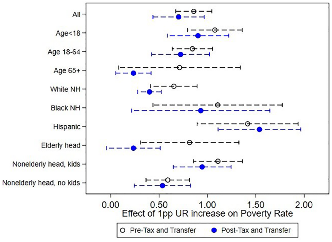
Comparison of Cyclicality of Individual Pre– and Post–Tax-and-Transfer SPM Poverty, by Subgroup

Finally, we expand our poverty measures to examine the impact of cycles on the broader distribution of income relative to poverty. Specifically, we run a series of models where the dependent variable is the share of persons who have post–tax-and-transfer resources below multiples of the SPM poverty threshold, ranging from 25 percent of poverty to 300 percent of poverty. Figure 4 plots the percent effects (dividing the point estimates by the mean of the dependent variable) of a 1 percentage point increase in unemployment rates on post–tax-and-transfer poverty along with their confidence intervals. The cyclicality of post–tax-and-transfer poverty rises sharply at the lowest income to poverty levels, peaking at income below 75 percent of poverty (reflecting a 7 percent increase for a 1 percentage point increase in unemployment). Above this point the cyclicality falls, such that at incomes below 275 or 300 percent of the poverty threshold, a 1 percentage point increase in unemployment leads to a 2 percent increase. Figure 5 extends this to present similar estimates for persons in the three household types. We find that across the lower end of the distribution, persons living in households headed by an elderly person (purple filled diamond) are significantly less affected by the cycle, and persons living in households with children and a nonelderly head (black filled circle) are the most affected. The percent effect peaks at about 9 percent for persons in households with children (at 75 percent of the poverty threshold) compared to 3 percent for persons in households headed by an elderly person (at 125 percent of poverty).

Figure 4

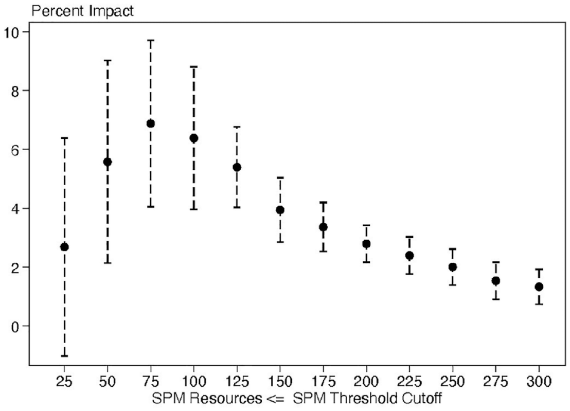
Cyclicality of Post–Tax-and-Transfer SPM Poverty by Cuts of Poverty, All Persons, 2000–2019

Figure 5

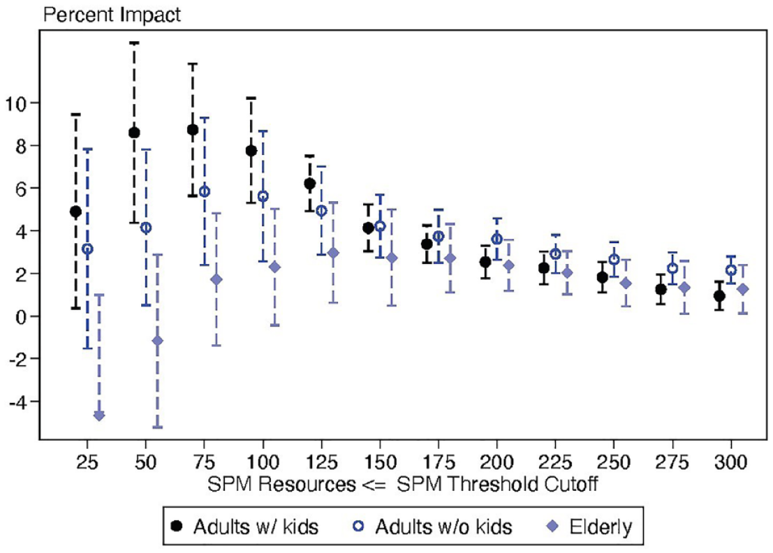
Cyclicality of Post–Tax-and-Transfer SPM Poverty by Cuts of Poverty, by Family Type, 2000–2019

Conclusion

This article, inspired by the work of Blinder and Blank (1986) and Blank and Card (1993), examines the impact of macroeconomic conditions on poverty. We update their work by studying the more recent period 2000 to 2019 (and 2000 to 2022) and by using the modern SPM championed by Becky Blank. We extend the previous work to leverage a more disaggregate unit of observation—state by year—to capture differences in the extent of the business cycle over place and across time. We find that SPM poverty is indeed relatively responsive to the business cycle after netting out state and year fixed effects, whether we use the unemployment rate or real median household income to measure the macroeconomy. We also replicate an important finding of this previous work, namely that taxes and transfers (both means-tested transfers and those stemming from the social insurance system) dampen the responsiveness of poverty in this era where the safety net is aimed more at in-work than out-of-work benefits.

Supplemental Material

sj-xlsx-1-ann-10.1177_00027162241289722 – Supplemental material for The Macroeconomy and Poverty

Supplemental material, sj-xlsx-1-ann-10.1177_00027162241289722 for The Macroeconomy and Poverty by Leslie McGranahan, Diane W. Schanzenbach, Marianne P. Bitler, Hilary Hoynes and Elira Kuka in The ANNALS of the American Academy of Political and Social Science

Footnotes

NOTE: Thanks to Hanns Kuttner, Diane Schanzenbach, and other conference participants for helpful comments. Thanks to Gaby Lohner and Raheem Chaudhry for excellent research assistance.

Supplemental Material

Supplemental material for this article is available online.

Notes

Marianne P. Bitler is a professor of economics at the University of California, Davis. Her work focuses on the U.S. safety net and the people who use it.

Hilary Hoynes is Chancellor’s Professor of Economics and Public Policy at the University of California, Berkeley. Her work focuses on the impacts of the social safety net in the U.S. for families with children.

Elira Kuka is an associate professor of economics at George Washington University. Her work focuses on understanding how government policies affect individual behavior and family well-being.

References

Bitler

Marianne

Hoynes

Hilary

. 2016. The more things change, the more they stay the same: The safety net and poverty in the Great Recession. Journal of Labor Economics 34(S1, part 2): S403–S474.

Bitler

Marianne

Hoynes

Hilary

Kuka

Elira

. 2017a. Child poverty, the Great Recession, and the social safety net in the United States. Journal of Policy Analysis and Management 36(2): 358–389.

Bitler

Marianne

Hoynes

Hilary

Kuka

Elira

. 2017b. Do in-work tax credits serve as a safety net? Journal of Human Resources 52(2): 319–350.

Bitler

Marianne P.

Hoynes

Hilary W.

Schanzenbach

Diane Whitmore

. 2020. The social safety net in the wake of COVID-19. Brookings Papers on Economic Activity 2020(2): 119–145.

Bitler

Marianne P.

Hoynes

Hilary W.

Schanzenbach

Diane Whitmore

. 2023. Suffering, the safety net, and disparities during COVID-19. RSF: The Russell Sage Foundation Journal of the Social Sciences 9(3): 32–59.

Blank

Rebecca M.

1993. Why were poverty rates so high in the 1980s? In Poverty and prosperity in the USA in the late twentieth century, eds. Papadimitriou

Dimitri B.

Wolff

Edward N.

, 21–57. London: Palgrave Macmillan.

Blank

Rebecca M.

2000. Fighting poverty: Lessons from recent U.S. history. Journal of Economic Perspectives 14(2): 3–19.

Blank

Rebecca M.

2008a. How to improve poverty measurement in the United States. Journal of Policy Analysis and Management 27(2): 233–254.

Blank

Rebecca

. 17 July 2008b. Why the United States needs an improved measure of poverty. Testimony in Establishing a modern poverty measure, before the Subcommittee on Income Security and Family Support of the House Committee on Ways and Means. 110th Cong., 40–47. Available from www.govinfo.gov.

10.

Blank

Rebecca M.

Blinder

Alan S.

. 1986. Macroeconomics, income distribution, and poverty. In Fighting poverty: What works and what doesn’t, eds. Danziger

Sheldon H.

Weinberg

Daniel H.

, 180–208. Cambridge, MA: Harvard University Press.

11.

Blank

Rebecca M.

Card

David

. 1993. Poverty, income distribution, and growth: Are they still connected? Brookings Papers on Economic Activity 1993(2): 285–339.

12.

Blank

Rebecca M.

Greenberg

Mark H.

. 2008. Improving the measurement of poverty. The Hamilton Project Discussion Paper 2008-17, Washington, DC. Available from www.brookings.edu.

13.

Blank

Rebecca M.

Ruggles

Patricia

. 1992. Using the Survey of Income and Program Participation to understand poverty and economic need. Journal of Economic and Social Measurement 18(1–4): 155–176.

14.

Bollinger

Christopher R.

Hirsch

Barry T.

Hokayem

Charles M.

Ziliak

James P.

. 2019. Trouble in the tails? What we know about earnings nonresponse 30 years after Lillard, Smith, and Welch. Journal of Political Economy 127(5): 2143–2185.

15.

Creamer

John

Shrider

Emily A.

Burns

Kalee

Chen

Frances

. 2022. Poverty in the United States: 2021. Current Population Report P60-277. Washington, DC: United States Census Bureau. Available from www.census.gov.

16.

Johnson

David

Levy

Helen

Matsudaira

Jordan

Wolfe

Barbara

Ziliak

James

. 2024. Measuring poverty: Advances to the Supplemental Poverty Measure. The ANNALS of the American Academy of Political and Social Science 711: 20–37.

17.

Larrimore

Jeff

Mortenson

Jacob

Splinter

David

. 2023. Unemployment Insurance in survey and administrative data. Journal of Policy Analysis and Management 42(2): 571–579.

18.

Meyer

Bruce D.

Mok

Wallace K.C.

Sullivan

James X.

. 2015. Household surveys in crisis. Journal of Economic Perspectives 29(4): 199–226.

19.

National Research Council. 1995. Measuring poverty: A new approach, eds. Citro

Constance F.

Michael

Robert T.

. Washington, DC: The National Academies Press.

20.

Short

Kathleen

. 2011. The research supplemental poverty measure: 2010. Current Population Reports P60-241. Washington, DC: United States Census Bureau. Available from www.census.gov.

21.

Wimer

Christopher

Fox

Liana

Collyer

Sophie

Garfinkel

Irwin

Kaushal

Neeraj

Laird

Jennifer

Nam

Jaehyun

Nolan

Laura

Pac

Jessica

Waldfogel

Jane

. 2023. Historical supplemental poverty measure data. New York, NY: Center on Poverty and Social Policy at Columbia University and Columbia Population Research Center. Available from www.povertycenter.columbia.edu.

22.

Wimer

Christopher

Fox

Liana

Garfinkel

Irwin

Kaushal

Neeraj

Waldfogel

Jane

. 2016. Progress on poverty? New estimates of historical trends using an anchored Supplemental Poverty Measure. Demography 53(4): 1207–1218.

Supplementary Material

Please find the following supplemental material available below.

For Open Access articles published under a Creative Commons License, all supplemental material carries the same license as the article it is associated with.

For non-Open Access articles published, all supplemental material carries a non-exclusive license, and permission requests for re-use of supplemental material or any part of supplemental material shall be sent directly to the copyright owner as specified in the copyright notice associated with the article.

0.00 MB

0.01 MB