Sage Journals: Discover world-class research

Abstract

Previous studies covering various developed countries suggest that changes in assortative mating by education have contributed only a little to the changes in income inequality, opposite to the expectations of many. In this paper we consider two potential reasons for the zero effects: (a) that it is the selection into partnership rather than assortative mating according to specific characteristics that matters; and (b) that for assortative mating to matter, a broader spectrum of matching characteristics than just education should be considered, such as matching by employment and social origin. We study these assumptions using register data on household income inequalities, education, employment and parental class background in Finland 1991–2014. We analyze men and women separately and focus on individuals aged 35–40. We concentrate on between-group income inequality as measured by the Theil index. The results suggest that partnership is an important factor behind income inequality, and changes in selection into partnership can explain a substantial part of the changes in income inequality. Assortative mating does not matter as much, even if more sorting characteristics are taken into account. Social origin contributes very little to the income inequality of families in Finland

Keywords

Income inequality assortative mating partnership social origin education unemployment

Introduction

Many influential social scientists have expressed their concern about growing social inequalities within and between societies in particular during the past decade (e.g., Milanovic, 2016; Piketty, 2014; Therborn, 2013). These observations appear to signal an important historical change. The early years of modernity were characterized by growing inequalities in income and wealth as well as other aspects of wellbeing, but broadly speaking the differences between key social groups had been steadily diminishing over the course of the 20th century. This progress seems to have reversed again during the last few decades.

Many studies considering the potential reasons for this reversal have focused on demographic and labour market changes. If one of the key issues in the income distribution of a society is the redistribution taking place within families (between family members), changes in family and employment composition may have a major impact on inequality (Sweeney and Cancian, 2004). Further, it has often been assumed that increasing assortative mating may have boosted inequalities, in particular with an increasing proportion of dual earner households (Blossfeld and Timm, 2003; Fernández et al., 2005; Schwartz and Mare, 2005). If like is more likely to mate with like, households with two high and two low income partners are likely to become more commonplace, thereby increasing income inequality between households in a society. With the assumption that there is income pooling (and redistribution) within households, the way that households are formed also becomes a key question for understanding income inequality between individuals.

Contrary to expectations, the overall conclusion of previous studies seems to be that assortative mating by education has contributed only little to the change in income inequality (e.g. Boertien and Permanyer, 2019; Breen and Andersen, 2012; Breen and Salazar, 2010). We consider two potential explanations for the null findings regarding assortative mating. First, while trends in assortative mating seem to vary considerably from country to country, the opposite is not true for partnership formation. Contemporary trends in cohabitation, delayed parenthood, separations and divorces, as well the growing life expectancy of the widowed have led to an increasing number of single adult households (e.g. Fokkema and Liefbroer, 2008; Lesthaeghe, 2010). The key issue behind changing levels of inequality may thus be not so much the assortative mating between different types of partners but who becomes partnered in the first place. Second, previous studies have almost solely considered assortative mating by level of education only. Yet other matching characteristics may also matter, such as employment and family background. Indeed, there are some indications that employment may be a key factor for explaining changes in income inequality (Zagel and Breen, 2019). The role of family background continues to be influential for adult attainment (Breen and Müller, 2020) as well as for assortative mating (Schwartz, 2013).

We study the composition of income inequality and changes therein in Finland during the period 1991–2014. We decompose the Theil index of income inequality, taking into account factors such as education, employment, parental class background, and partnership. After establishing the main components of inequality, we consider the extent to which they explain the changes in inequality during the covered period. Although we concentrate on household income inequality by using equivalised household income, we conduct our analyses at the individual level in order to properly take into account the importance of selection into partnership.

Income inequality and assortative mating

It is well established in the literature that who marries whom is reflected in socioeconomic inequalities between households (Blossfeld and Timm, 2003; Kollmeyer, 2013; Raaum et al., 2008). Contemporary trends in the rising level of education and the increasing importance of dual earnership for economic wellbeing has led to an expectation that the link between assortative mating and income inequality is changing. Related to this, concerns about increasing educational homogamy have led a number of previous studies to consider the extent to which assortative mating and changes in its strength have contributed to changes in income inequality. The overall conclusion of these studies seems to be that while a link between assortative mating and income inequality can often be found, changes in the former do not seem to contribute much to changes in the latter (Boertien and Permanyer, 2019; Schwartz, 2013).

Other related factors seem to be more decisive, although they seem to vary considerably from one context to another. For instance, Breen and Salazar (2010) found that the key issue for change in inequality in Britain from 1979 to 2000 was the change in the distribution of family earnership types, i.e. whether families have dual earnership or single male or female earners. For the US, the same authors found that assortative mating actually reduced income inequality from the 1970s to 2000s, opposite to the common assumption (Breen and Salazar, 2011). More recent analyses for the US by Zagel and Breen (2019) suggest that women’s improving education level and changes in men’s employment contributed to the changes in income inequality from the 1990s to the 2000s. Eika and colleagues (2014) concluded somewhat similarly in their comparison of the US and Norway that the growing returns to education and the consequent increases in income inequality were mitigated partly by the rising education level of women.

For Denmark, Breen and Andersen (2012) found that the changes in assortative mating from 1987 to 2006 contributed to an increase in the Theil index of income inequality of up to 7%. The strengthening association between income inequality and assortative mating was nonetheless entirely attributed to changes in men’s and women’s marginal distributions of education. The authors argue that due to the welfare state and regulated labour market, there might be less within educational group variation in social democratic welfare states, which then makes educational inequality more tightly connected to income inequality. If indeed these factors are decisive, similar patterns may also be observed in Finland.

The link between assortative mating and household income inequality seems rather obvious and the null findings unexpected. Schwartz (2013) speculates on three potential reasons for the results: first, that the changes in assortative mating have been too small to observe an effect; second, that homogamy varies too much across education levels to show in overall inequality; and third, that the finding might result from the weak association between women’s education and earnings. These assumptions seem to be refuted by more recent findings. Based on simulations of 21 counties in the LIS database, Boertien and Permanyer (2019) conclude that even if educational homogamy were maximized, it could not contribute much to income inequality in these countries. If this is the case, the first two explanations would not be crucial. Further, the above cited findings of Eika and colleagues (2014), finding income inequality to be mitigated partly by the rising education level of women, suggest that at least the link between women’s earnings and education is strong enough to actually reduce income inequality in some country contexts. So alternative explanations for null findings are required.

Selection into partnership

One-person households are considered as the fastest growing type of households globally (Esteve et al., 2020; Yeung and Cheung, 2015). This is linked to an increasing number of widows due to increased longevity, later occurring family formation, increasing economic independence due to growing economic prosperity and female labour market attachment as well as overall improvements in human development. To put it simply, people are more likely to find themselves as being single, can afford to live so better than before, and may even prefer the independence associated with it. Previous studies have already established that the growing proportion of single households has contributed to income inequality (Bloome, 2017; Burtless, 1999; Kollmeyer, 2013).

At the same time, selection into being partnered seems to have changed. During the second half of the 20th century, higher education, better labour market attachment and a high income have all begun to matter more for union formation for both men and women. The evidence suggests that this advantage in selection was evident in the Nordic countries already before the mid-1990s (Bertrand et al., 2016; Jalovaara, 2012; Van Bavel et al., 2018). The never partnered are likely to be low educated and have low income and weak labour market attachment (Jalovaara and Fasang, 2017, 2020).

Some studies have touched upon the potential importance of increasing single-headed households for the changes in the income distribution. The analysis of Breen and Andersen (2012) already hinted at the importance of this change; the change in the distribution of singles contributed to income inequality much more than the change in assortative mating among those who partnered. Yet the authors concluded that this was mainly driven by the overall change in educational distributions. Further, Zagel and Breen (2019) concluded that for West Germany, family demographic changes, indicated by the number of single and dual headed households with or without children, contributed to the change in income inequality.

One of the potential explanations why the importance of selection into partnership has not been considered more often in the previous literature is its focus on the partnered or on households as the main unit of society. For anyone studying inequality in a society, the focus on couples is a peculiar choice. While the majority of adults are indeed either cohabiting or married, for substantial parts of their adult lives in contemporary societies they typically are, in fact, singles. Additionally, the contribution of relevant aspects of family dynamics may be entirely missed. For instance, if single parents are excluded, we are likely to underestimate inequality among women, as single parents are particularly likely to be low income (Nieuwenhuis, 2020). Similarly, excluding singles reduces observed inequality among men, as particularly low educated men tend to remain single (Jalovaara and Fasang, 2020).

While taking single-headed households into account is certainly a better choice than excluding them altogether, focusing on households is still problematic. First, in the income distribution of households, singles would get a double weight as compared to the coupled, overpopulating the lower end of the strata with singles, if compared to the population of individuals. Second, and perhaps more importantly, while one may argue that a society can be considered as consisting of different kinds of households, most would probably agree that inequality between households is societally relevant only if that is properly reflecting the inequality among individuals.

From the point of view of empirical application, however, the distinction between focusing on households instead of individuals is small. Most income datasets are based on samples of individuals, rather than of households. This in practice removes the problem of the overpopulation of singles. Moreover, while the studies typically refer to family incomes, the income to be considered is not really the total within families or households but rather the assumed family-structure adjusted individual share of family income. This is done by applying different kinds of equivalence scalings to the total sum of the income of the family, taking into account for instance the number of adults and children. The reasoning behind this adjustment is clear: due to lower shared costs of living for those with spouses and the added economic burden of taking care of the underage children, researchers should take into account the economies of scale in consumption within households (Brandolini and Smeeding, 2011; Buhmann et al., 1988).

In our case, although we theoretically prioritize individuals as the main unit of analysis over families or couples, we follow the same strategy: our individual level income measurement is a similarly computed individual share of the total family income. Jenkins and Lambert (1993) note that this requires the additional assumption that family members share all of their incomes (see also Ebert and Moyes, 2017). This is something that does not always occur in real life due to different needs, normative differences in how the living expenditures should be shared, and the varying power relationships between family members (cf. Bennett, 2013). In practice, however, there are no good ways around the problem, apart from just noting that the inequality observed refers to the hypothetical inequality that would prevail, if the incomes were shared.

While the focus on individuals instead of households could be justified due to epistemological reasons, the most important reason for us is that the selection into partnership can only be considered in our analyses if we also include the non-partnered population. An additional advantage is that it allows analyzing inequality among men and women separately. Indeed, based on numerous studies on different types of socioeconomic inequalities and demographic behaviour (e.g., Buchmann et al., 2008; Lee and Solon, 2009; Prix, 2009), it seems reasonable to assume that the mechanisms contributing to inequality may be different for men and women.

In our case, we assume that selection into partnership is likely to matter more for inequality between women than between men. This is because even in relatively egalitarian Finland, women’s average earnings are up to 16% percent lower than those of men (Statistics Finland, 2018), thus the economies of scale within the family should have a stronger influence on inequality among women.

Multiple types of assortative mating

Our second assumed explanation for null findings for the contribution of assortative mating on income inequality is the fact that assortative mating can take place in different forms. The studies on partnership homogamy have traditionally focused on matching by education, less often on other forms of social stratification, such as occupational standing or social class. Usually the association has been assumed to be the strongest in the case of education, somewhat weaker in the case of occupation and lowest in the case of social class (Kalmijn, 1991, 1998). However, as also noted by Kalmijn, individuals tend to belong to several groups at the same time and “making a match in one respect implies forgoing a match in another” (Kalmijn, 1991: 497). Thus, even if partnership selection by education does not change in a way that would contribute to the change in income inequality, the opposite may very well be true if the matching takes place based on other characteristics.

Here we focus on two other contributors for partnership matching: employment and parental background. The findings of Zagel and Breen (2019) suggest that the changes in men’s employment in particular contributed to the change in income inequality in Germany. Unemployment is, however, also a well-known risk factor for separations (Jalovaara, 2013), so it may actually be one of the reasons for selection into partnership as well as away from them. There is also some evidence indicating that unemployment may play a role as a form of assortative mating contributing to income inequality as well: when both partners are unemployed, re-employment appears to be particularly hard, thus contributing particularly strongly to the income of those households (Bacon et al., 2014; Miller, 1997).

The importance of family background for inequalities in income is well and widely established in the literature, also in the context of egalitarian Nordic countries (e.g. Aaberge et al., 2002; Sirniö et al., 2013). Yet its relation to the association between assortative mating and the income distribution has not been studied previously, although it is sometimes discussed (e.g. Schwartz, 2010). While a stronger importance of family background may be assumed to lead to greater inequality as such, part of that effect can be mediated both by contributing to the selection into partnership as well as by assortative mating (Kailaheimo-Lönnqvist et al., 2019; Raaum et al., 2008).

The country context

The period of 1991–2014 in Finland fits the purposes of our research questions well. Figure 1 reports the often-used Gini and Theil inequality indices during the period according to both gross and net income. The figure also distinguishes inequality in the full population (available from Statistics Finland, 2021) as well as in our target population, age 35–40. The period includes growth of income inequality until 2000 and then a slowly diminishing trend towards 2014, in our target population especially since 2003 or 2008, depending on the measure used. The steep economic crisis of 1991–1995 hardly shows in the development of income differences. The growth in income inequality during the 1990s has been mainly attributed to weakening redistribution rather than changes in, for example, earnings (Blomgren et al., 2014). Despite the increase in the 1990s, income inequality in Finland has remained at a comparatively low level throughout the period. It also seems that the changes in inequality have been smaller in our target population than in the population in general.

Figure 1.

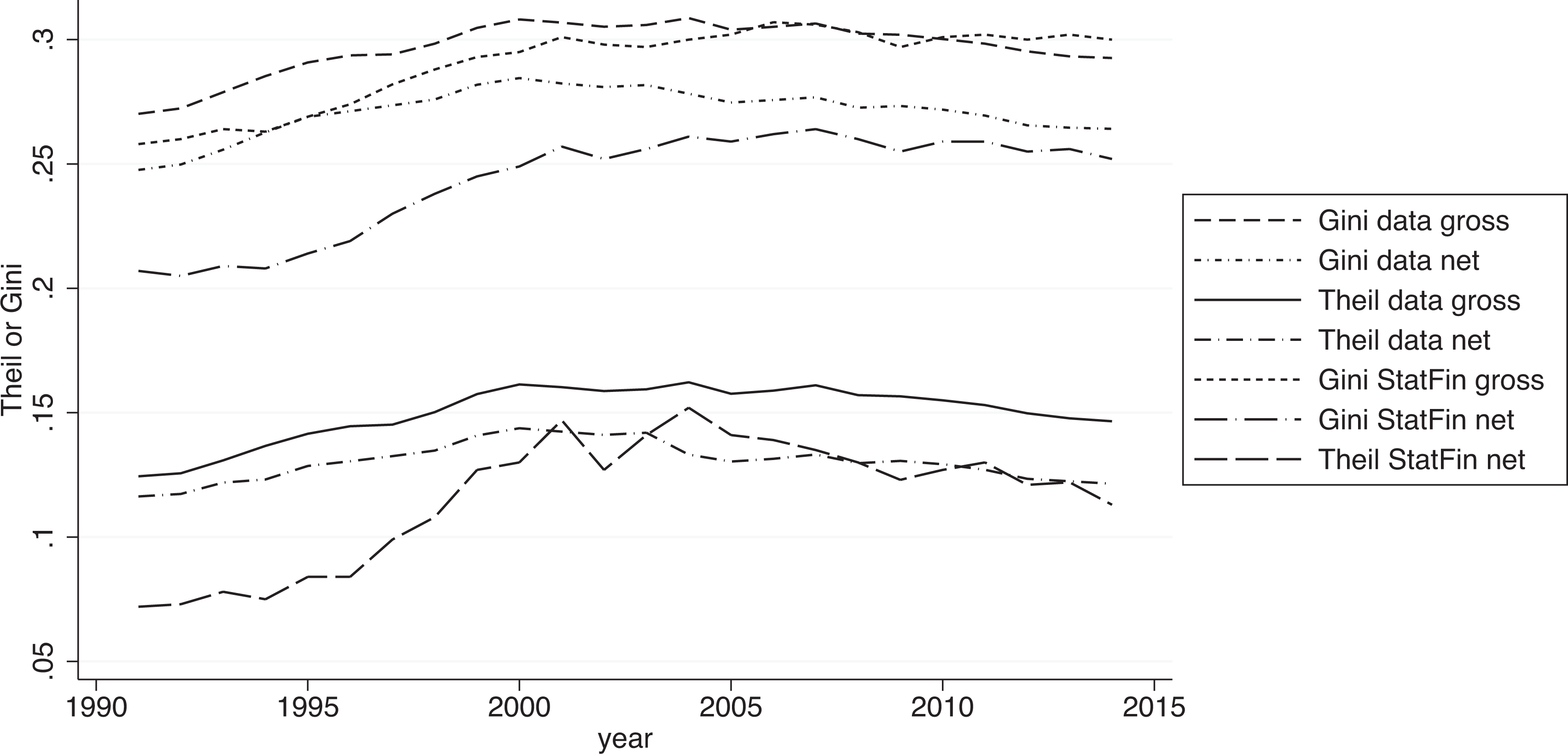
Income inequality in Finland, 1991–2014. Gini and Theil indices from our sample (ages 35–40, “data”) and the full population information from Statistics Finland (“StatFin”), gross and net incomes. Full population data source: Income distribution statistics, Statistics Finland, 2021.

Figures 2 and 3 show the changes in some other characteristics of the target population. Interestingly, the period as a whole is characterized by continuous educational expansion, affecting the proportion of highly educated particularly in the second half of the period. Educational expansion has taken place especially among women: 40% of women in our sample had tertiary education at the end of the period, in contrast to 32% of men. In 1991 men were still better educated than women. The key factor behind the rapid change has been the introduction of polytechnics in the mid-1990s, providing bachelor level degrees and replacing the prior post-secondary institutions in popular fields of education (such as engineering and nursing).

Figure 2.

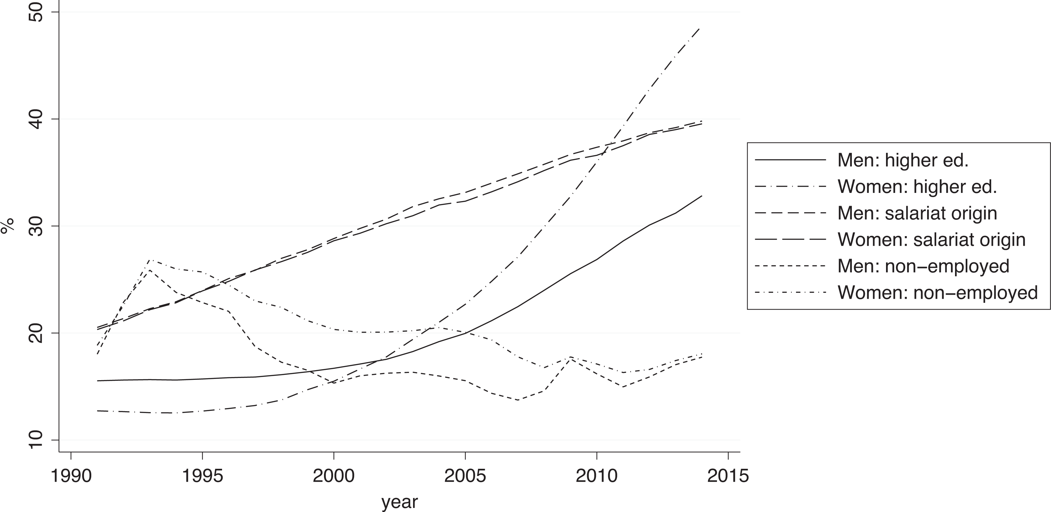
Percentage of tertiary-educated, non-employed and those with salariat class parents (EGP I-II), men and women age 35–40.

Figure 3.

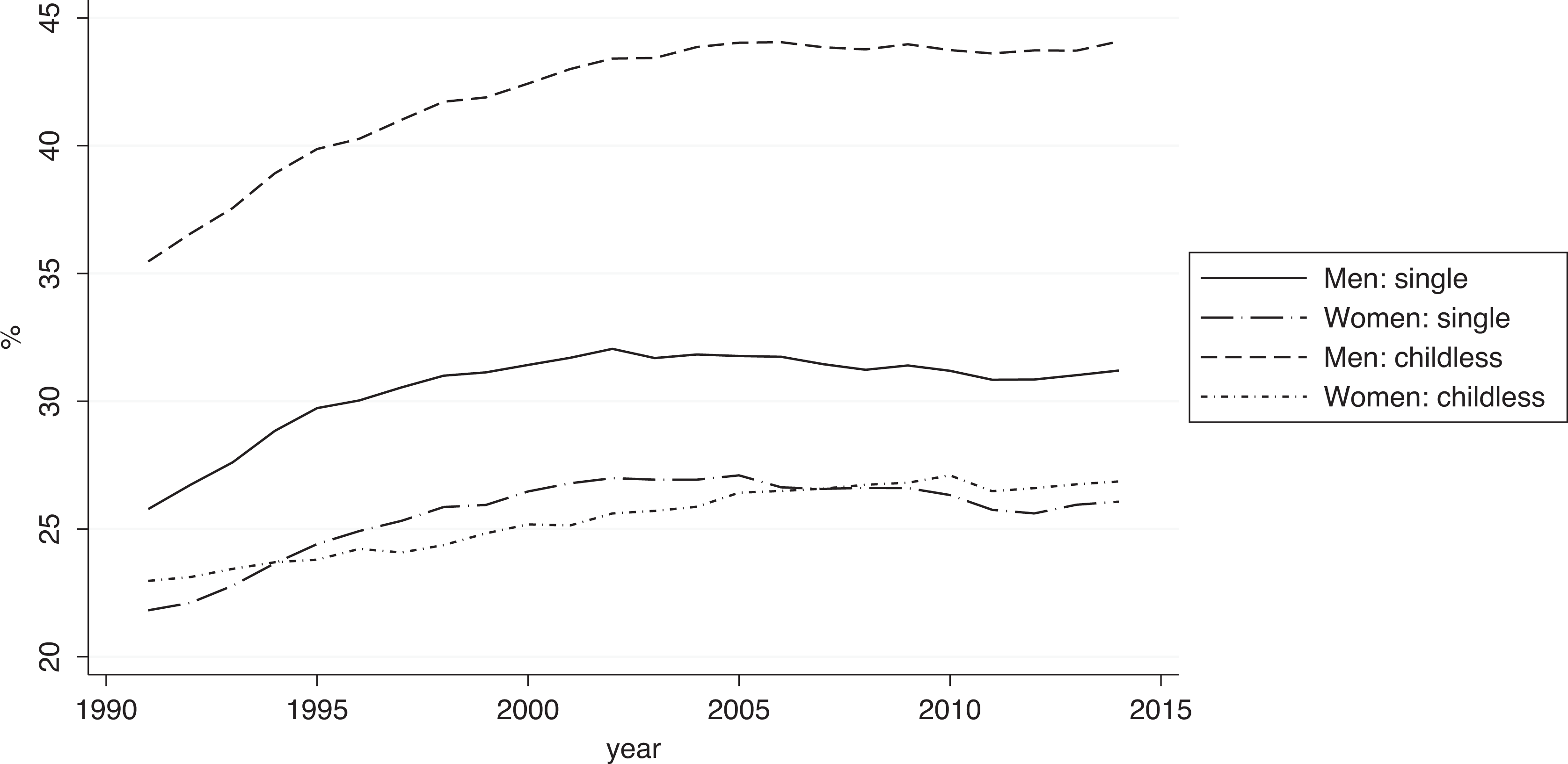
Percentage of singles and childless, men and women age 35–40.

Parental class background also improved over the whole period. The proportion of those with service class parents more than doubled during the period, a substantial change that has largely been missed in the contemporary discussion on fundamental changes in society. As expected, the non-partnered population grew as well (Figure 3), but only over the first half of the period, and then remained steady at the same level. The pattern of childlessness mirrors that of non-partnering albeit at a lower level. Interestingly, of all these indicators, the pattern of change in partnership (as well childlessness) resembles the change in inequality the most.

Finally, Figure 2 also reports the proportion of non-employed. While Finland went through a severe economic crisis during 1991–1995, the growth in non-employment in this age group had begun already earlier. The level of non-employment never returned to the post-recession level, and in fact was even reduced during the global economic recession that began in 2008. Perhaps surprisingly, the changes in non-employment do not seem to be reflected in similar changes in income inequality.

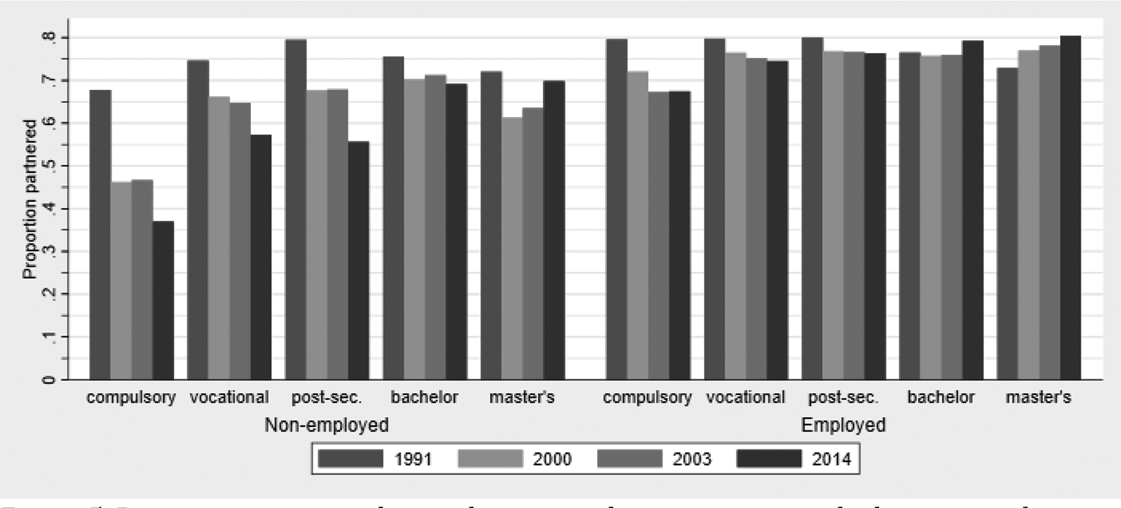
Figures 4 and 5 show that partnership propensity according to level of education and employment for men and women. The probability of being partnered reduced within all groups over the period 1991–2014, with the exception of tertiary-educated employed women. The reduction was greatest among those who were both low educated and non-employed. At the beginning of the period, women’s partnership propensity was relatively equal regardless of education level or employment status, whereas by the end of the period, they were relatively similar to men in terms of an educational gradient favouring the higher educated as well as an ‘employment premium’. Overall, it seems that the link between partnership and the association between education and employment changed during the period.

Figure 4.

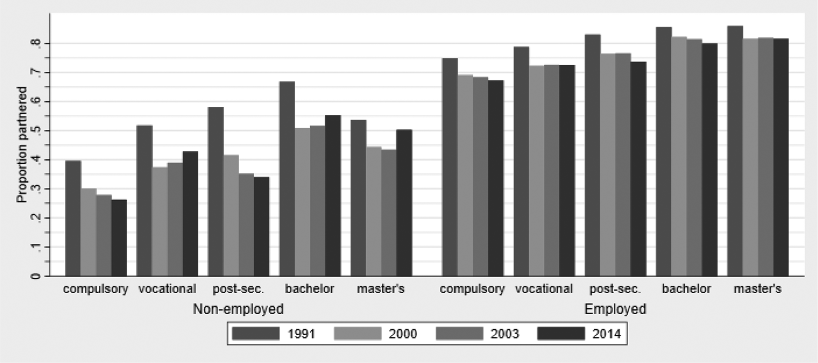
Proportion partnered according to employment status and education in the years 1991, 2000, 2003, 2014. Men aged 35–40.

Figure 5.

Proportion partnered according to employment status and education in the years 1991, 2000, 2003, 2014. Women aged 35–40.

Outside the information provided by these figures, there are some interesting patterns to note in the changes in the associations related to assortative mating. The data show that Spearman’s rho (correlation) between spousal education levels was around 0.43 in the beginning of our follow-up and declined steadily to just under 0.41 around the turn of the century and then rose again to approximately 0.44. The proportion of educationally homogamous couples (at the same level of education) remained steady at about 40%. At the same time, the correlation between own income and spouse’s income was extremely small (at most 0.08) in our sample.

Data and methods

We use a register-based Finnish Growth Environment dataset. It is based on a 10% sample of the Finnish population of 1980 that is matched with their children. The children are matched with all their cohabiting and married spouses across their lifecourses, and all the spouses are matched with their parents. This allows us to include both cohabiting and married couples and to study the importance of matching by parental characteristics. The annual tax register data on disposable income are available from 1991 onwards. This allows us to follow how income inequality changes among the households of 35–40-year-old Finns between 1991–2014; for older age groups we would not be able to match respondents and their spouses reliably to their parents during the entire covered period (information available only from 1970 onwards) and the younger ones would not have reached the occupational maturity or have gone through key stages of family formation. With these restrictions, our annual samples include information from approximately 64,200–76,200 men and women.

The data provide yearly information on all taxable net income all individuals have acquired during the covered period. The coverage of the different sources of income is generally considered as very good, but excludes certain non-taxable income sources, such as last resort social security benefits and child support payments.

As explained above, we focus on individual incomes computed from the total household income using equivalence scaling. In order to do this, we sum up all annual taxable incomes of the ego and the possible spouse and divide the produced aggregate income using the chosen scale. We apply the square root equivalence scaling (OECD, 2012), where the total household income is divided by the square root of the number of family members. This is one of the most often-used methods of equivalence scaling but it differs slightly in its assumptions from the also often-used OECD-modified scaling, according to which the children are assumed to have considerably lower consumption needs than adults (0.3 weight of each child, contrasted with the weight of 1 for the first adult and 0.7 for the second).

The level of education for both the ego and the possible spouse has five levels: (1) compulsory schooling, (2) vocational secondary, (3) general secondary, post-secondary and short cycle tertiary education, (4) bachelor’s degrees and (5) master’s degrees or higher. The information on the highest degree acquired is updated annually.

Among the parents, the educational distribution is still relatively compressed due to the low general level of education among these cohorts. In order to observe more variance in parental characteristics, the status of the parents (of both the ego and the possible spouse) is measured according to five levels of EGP classes: I higher service; II lower service; IIIa + V & VI high grade routine non-manual, manual supervisors and skilled workers; IV the self-employed; and IIIb + VII low-grade routine non-manual and unskilled workers. We use the dominance principle to choose between mother’s and father’s class from the latest available year prior to the year of measurement.

The variables related to employment, being single (or partnered) and having children are coded as dummies. These statuses are measured on a single date at the end of a given year.

We use the Theil index to analyze the factors contributing to income inequality. This index is less sensitive to changes at the top and bottom than many of the other alternative income inequality measures. Despite the relative robustness of the measurement and fairly sizeable data, we needed to drop the top one percentile of the income distribution to provide consistent estimates (in these analyses our annual datasets have information from 63,600–75,400 individuals). Perhaps the greatest advantage of the index, however, is that it can be decomposed into between and within inequality across the population subgroups.

The equation for the Theil index is

T = \frac{1}{n} Σ_{i = 1}^{n} \frac{x_{i}}{\bar{x}} l n (\frac{x_{i}}{\bar{x}})

In our case, this stands for the average ratio of income of an individual x_i to mean income $\bar{x}$ , multiplied by the log of the same quantity, with n denoting the number of individuals.

The index decomposes into between and within-group inequality:

T = Σ_{j} p_{j} \frac{{\bar{x}}_{j}}{\bar{x}} l n (\frac{{\bar{x}}_{j}}{\bar{x}}) + Σ_{j} p_{j} \frac{{\bar{x}}_{j}}{\bar{x}} T_{j}

Population subgroups are indexed by j, ${\bar{x}}_{j}$ stands for the mean income of a subgroup and p_j is the proportion of individuals in a subgroup (population share). According to the first part of the equation, between-group inequality can be measured as a logarithm of the ratio of the subgroup j mean income to the overall mean income. According to the second part, within-group inequality is based on the summed Theil indices of each subgroup, T_j , each weighted by the group’s proportional size and the group’s share of income.

We conducted the analyses in three parts. As a first step, we simply considered how much between-group inequality there is when taking each factor separately. This provides us a good understanding about the overall importance of the different factors. In this step, we do not test the attributes of the spouse as these are conditional on being partnered and thus they are an additive rather than a separate factor.

As a second step, we additively test the joint contributions of the factors. We begin by first only taking into account the factor contributing to inequality the most (from the previous step), then test which factor adds the most to this and take this into account, and so forth until we have added all the different factors. Once partnership is included, we also begin testing the contribution of the spouse’s characteristics. This procedure is followed separately for men and women. We only show the results for the final estimates rather than all the tests at each stage. When analysing the factors separately, as is done in the first step, their joint contribution cannot be assessed and the way that they overlap is not taken into account. On the other hand, some factors only become important in combination with another factor (as will be shown for the case of children). Additionally, the characteristics of the spouse can only be taken into account after partnering is also included, otherwise this inflates the role that the spouse’s characteristics play. In both the first and the second step, we calculate confidence intervals with bootstrapped standard errors (Liao, 2016).

As a final step, we provide counterfactual estimates on how much inequality would have changed between different time points, changing only one element at a time and keeping the other key characteristics of the target population constant. We do this for the period of increasing inequality, 1991–2000, and decreasing inequality, 2003–2014. In these analyses we use the three factors found to be the most important for income inequality in the previous two steps of the analyses (and in the online appendix for the four most important factors). The counterfactuals are derived by taking the three components of the Theil index (p_j , ${\bar{x}}_{j}$ and $T_{j}$ ) from the first year and, one at a time, replacing them with the value from the later year, and then recalculating the three measures of inequality.

Because we are particularly interested in selection processes, we analyze further the change in the population shares ( $p_{j}$ ). Changing population shares consist of two processes: changing marginal distributions and changing associations between different factors. We focus on the changing associations. In order to do this, we follow the examples of Breen and Salazar (2010, 2011) and Boertien and Permanyer (2019) and use the Deming-Stephan algorithm. This means that we (iteratively) change the association between the most important factors from the first year to match that of the later year, while keeping the marginal distributions constant. This gives us an estimate of the contribution of changing associations separately from changes in the marginal distributions. We describe this more concretely in the results section.

As mentioned above, we conduct all our analyses separately for men and women. The online appendix reports analyses for men and women together.¹

Results

Figure 6 reports the between-group income inequality according to single indicators among men, Figure 7 among women. For men, employment is clearly the strongest contributor, rising during the early years of the 1990s and remaining at a high level until the end of the period. Between-group inequality according to employment is almost double that of the other two important factors, namely education and having a partner. For men, the contribution of education becomes somewhat more important than being partnered in the late 1990s and remains so until the end of the follow-up. Both having a child and family origin matter very little for men’s income inequality.

Figure 6.

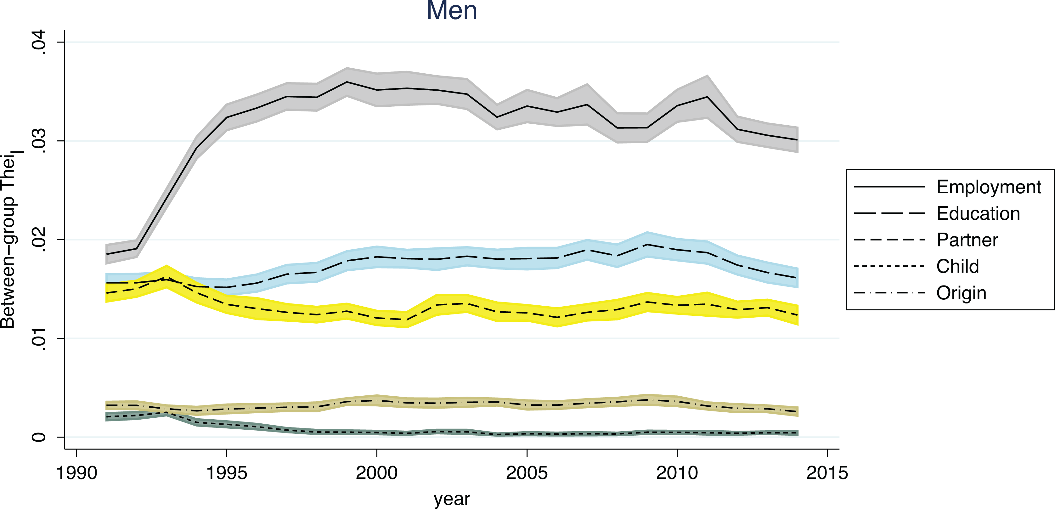
Between-group Theil index by each variable individually. Men age 35–40.

Figure 7.

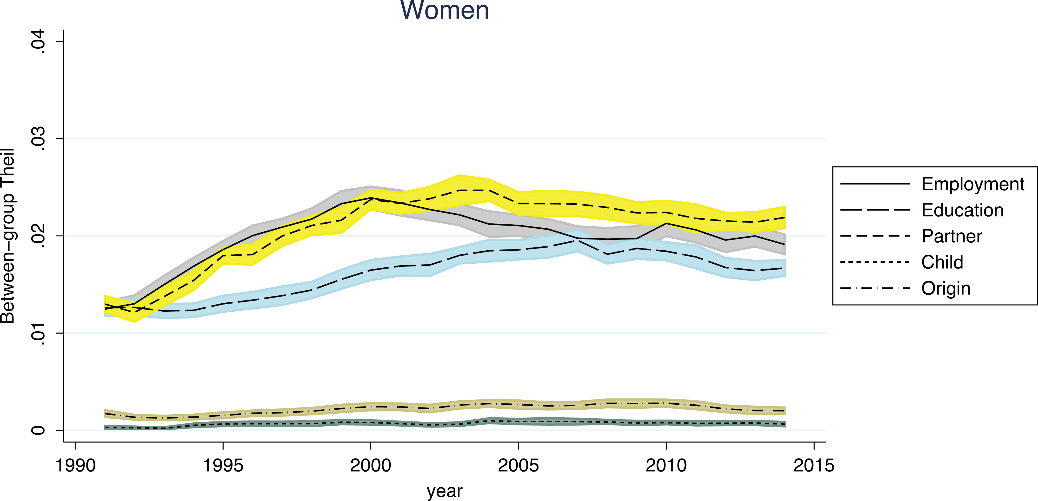
Between-group Theil index by each variable individually. Women age 35–40.

For women, the patterns are surprisingly different. The importance of being partnered and employed both increase throughout the 1990s more or less hand in hand. However, since 2000, between-group inequality according to employment diminishes while the importance of partnering continues to grow for a few years longer. Overall, being partnered is more important for between-group inequality among women than among men. The role of education slowly becomes more important for women until 2005. Since then, the importance of being partnered, employed and education are relatively close to each other. Similarly, to men, having a child and family origin matter very little.

We next move to the results of combining variables, reported in Figures 8 (men) and 9 (women). For men, we start from employment, then add one by one (in the order in which they contribute the most) education, being partnered, having a child, assortative mating by spouse’s employment and then by spouse’s education. The results indicate that quite clearly, the changes in income inequality mostly originate from the changes in employment. The additional contributions of other factors are almost constant over time. Although having children had a minimal influence on producing between-group inequality alone, it has more of an impact in combination with the other factors. Adding spouses’ characteristics adds very little to the big picture, and in fact the between-group Theil does not grow significantly when spouse’s education is added to the model. As was already evident from the previous step, origin contributes minimally to between-group inequality, and our unreported analyses here confirm this. This also applies to spouse’s origin.

Figure 8.

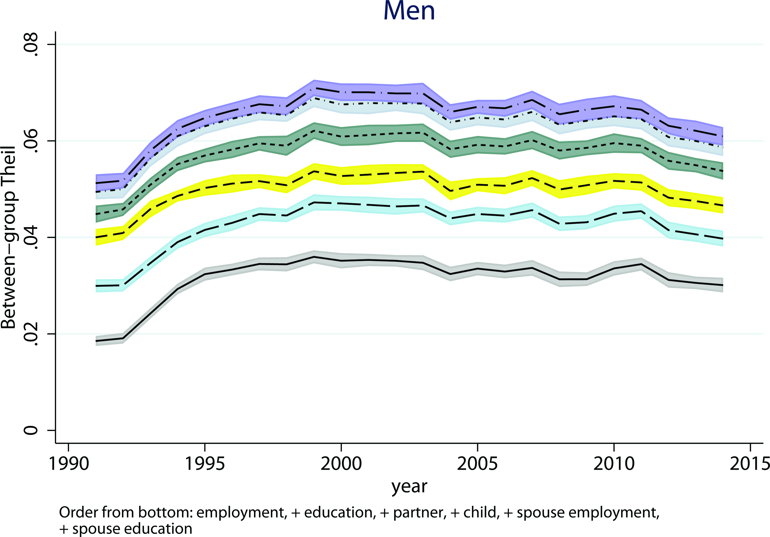
Between-group Theil index, accumulation by combinations of variables. Men age 35–40.

Figure 9.

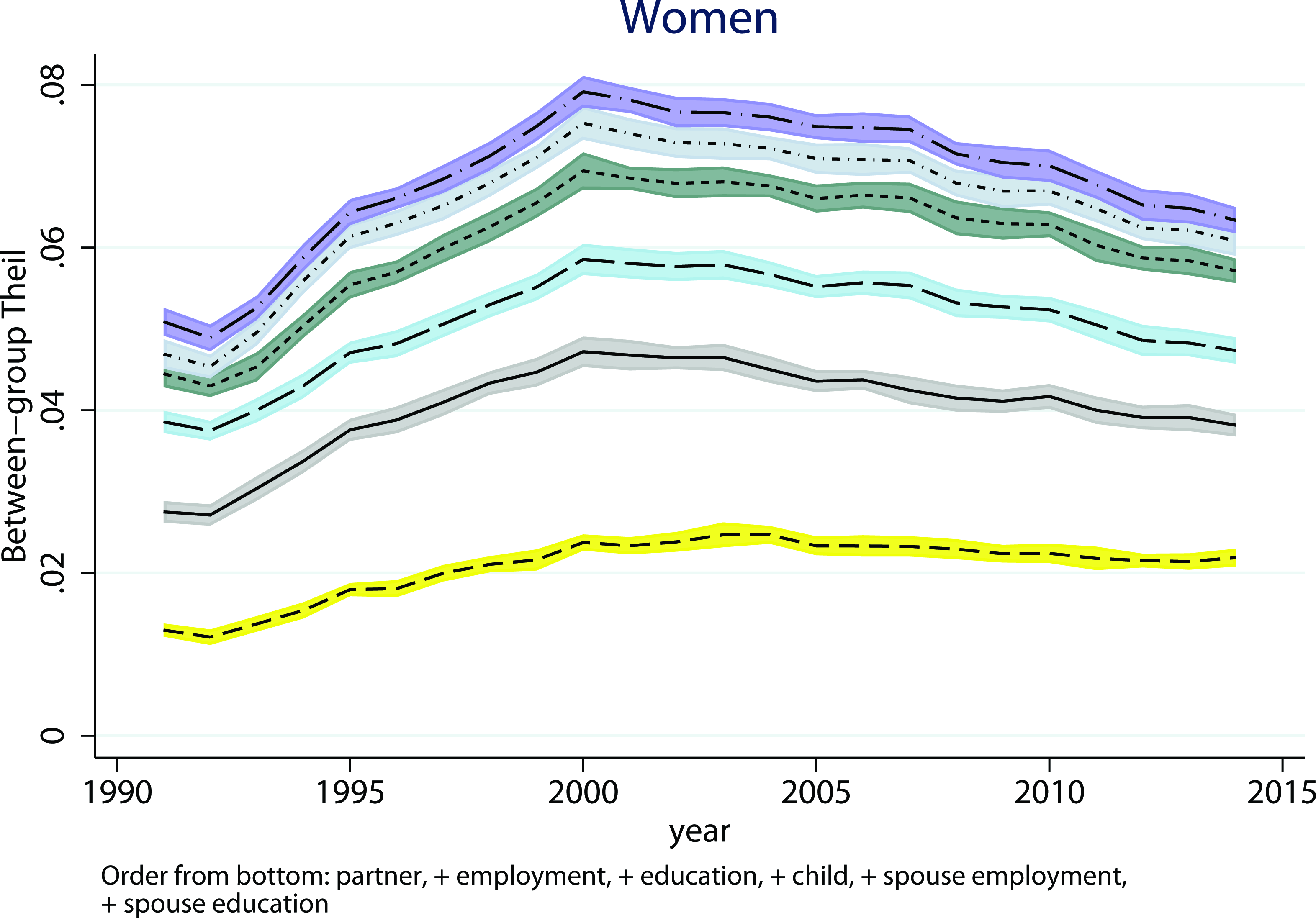
Between-group Theil index, accumulation by combinations of variables. Women age 35–40.

For women, the story is again somewhat different. Based on the results reported in Figure 7 it was concluded that being partnered was the factor that produced the most between-group inequality among women. However, employment seems to contribute roughly as much, and both of these seem to contribute to the change in between-group income inequality. The additional importance of education seems to be more or less at the same level as for men, whereas having children clearly contributes more to income inequality among women. In fact, it seems that the contribution of children grew until 2000, i.e., until the overall income inequality grew (in Figure 1). The importance of spouse’s characteristics is very similar as in the case of men: assortative mating contributes fairly little to between-group inequality and spouse’s employment is somewhat more important than spouse’s education. Similarly, as for men, own origin and spouse’s origin hardly contribute at all (not shown).

Finally, Table 1 reports our counterfactual results where we use employment, education and partnership as the factors defining between-group inequality. The upper part of the table shows the estimates for the changes in Theil, between-group and within-group inequality for 1991–2000, the lower part between 2003–2014. We continue our focus on between-group inequality and start with the basic counterfactuals. Changing mean earnings of different population groups seems to have been a strong component of change for men in both periods. For instance, if only the mean earnings had changed, the counterfactual change for men between 1991–2000 would have been 33%, whereas the true observed between-group change among men during that period was 32%. This is also the case for women in the second period, whereas in the first period, changing population shares seems to have contributed equally. When it comes to the overall Theil, changes in within-group Theil seem to have been an even slightly larger contributing factor for both men and women and in both periods.

Table 1.

Counterfactual contributions of within-group Theil, mean earnings, population shares, and the association between education, employment and partnership on the changes in inequality in Finland. Changes between periods 1991–2000 and 2003–2014, separately for men and women.

	Men						Women
	Theil	% change from first year	Between	% change from first year	Within	% change from first year	Theil	% change from first year	Between	% change from first year	Within	% change from first year
1991–2000
Basic counterfactuals
1991 observed	0.1216		0.0400		0.0816		0.1107		0.0386		0.0721
Change within	0.1358	12	0.0400	0	0.0958	17	0.1229	11	0.0386	0	0.0843	17
Change mean earnings	0.1321	9	0.0534	33	0.0787	-4	0.1166	5	0.0463	20	0.0703	-3
Change pop shares	0.1229	1	0.0407	2	0.0823	1	0.1227	11	0.0488	26	0.0739	2
2000 observed	0.1444	19	0.0527	32	0.0917	12	0.1429	29	0.0585	52	0.0844	17
Decomposing distribution of p (pop share)
Change associations	0.1430	18	0.0513	28	0.0916	12	0.1358	23	0.0517	34	0.0841	17
2003–2014
Basic counterfactuals
2003 observed	0.1441		0.0536		0.0905		0.1395		0.0579		0.0816
Change within	0.1322	-8	0.0536	0	0.0786	-13	0.1327	-5	0.0579	0	0.0748	-8
Change mean earnings	0.1373	-5	0.0448	-17	0.0925	2	0.1319	-5	0.0484	-16	0.0835	2
Change pop shares	0.1458	1	0.0568	6	0.0890	-2	0.1355	-3	0.0581	0	0.0774	-5
2014 observed	0.1246	-14	0.0466	-13	0.0780	-14	0.1181	-15	0.0473	-18	0.0708	-13
Decomposing distribution of p (pop share)
Change associations	0.1255	-13	0.0475	-11	0.0780	-14	0.1147	-18	0.0436	-25	0.0711	-13

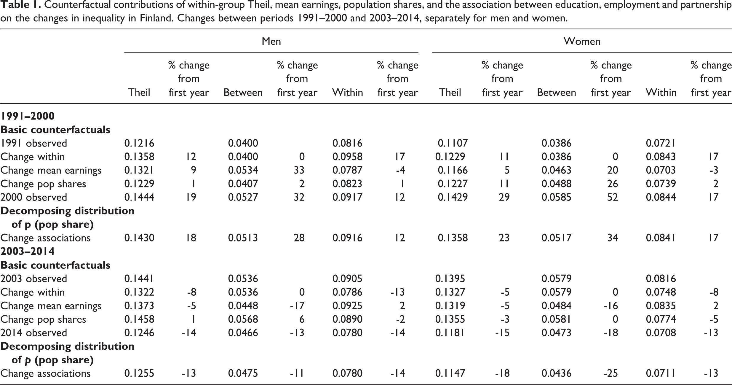
Interestingly, the relatively small influence of changing population shares seems to have actually masked two contradictory trends. For the second counterfactual, we assume that only selection into partnership changed; we thus change the association of education and employment (combined) with partnering, while keeping the marginal distributions of these three constant. In other words, the association between education and employment is also kept constant and only the association between partnering with a categorical variable combining education and employment is changed. In addition, within-group Theil and mean earnings are kept constant. This also seems to match the observed change in both periods rather well for both between-group Theil as well as the overall Theil – particularly for men. For example, in the first period the real Theil for men in 2000 was 0.144 (up from 0.122 in 1991) and the counterfactual produced a Theil of 0.143. For women in 2000 the real Theil was 0.143 (up from 0.111 in 1991) and the counterfactual produced a Theil of 0.136.

In other words, in a world where everything else was the same as in 1991 (or 2003) but only the association of partnering with education and employment were as in 2000 (or 2014), we would expect income inequality to be almost the same as in 2000 (or 2014). Interestingly, as we did not see this when we changed all population shares (with the partial exception of women 1991–2000), it seems that the changes in the marginals (covering distributions of partnered, education or employment and all combinations of these variables) must have included also changes that counterbalanced the effects of selection into partnership alone. Overall, the findings reported in the table provide further evidence that changes in income inequality have to a certain extent been driven by the changing selection into partnership, both by education and employment.

Figures 4 and 5 shed some further light on these results. In the first period, partnering and the combination of employment and education became increasingly positively related, increasing inequality. On the other hand, the changes in these associations in the second period was in many cases dissimilar to the changes in the first period. Although it is difficult to pinpoint the exact cause for the change, we believe that the educational changes in who partners within the group of non-employed individuals may be an important factor in combination with the strongly rising proportion of highly educated and strongly diminishing proportion of the very lowest educated even within both the non-employed and the population of singles. This means that being disadvantaged according to partnership status is less strongly associated with being disadvantaged according to employment within a group that is both increasing in size and relatively advantaged otherwise (i.e. the highly educated).

The results were replicated in men and women combined, using gender as one of the factors potentially contributing to income inequality. These results are reported in the online appendix. They show that the overall trends are an average of the trends for men and women. In addition, when using equivalised income, gender contributes less to income inequality than employment, partnership, education, children, partners’ education and employment. Adding children to the counterfactuals reported in Table 1 did not substantially influence our conclusions, although it is clear that children (in combination with partnership) contribute to inequality particularly among women and there has been change over time in how this is related to education and employment.

The analyses reported in the main text were also replicated using gross income. They did not differ substantially from the ones reported here. We also conducted auxiliary analyses using individual incomes without equivalization. In those analyses, partnering does not influence the overall income inequality much. This is not surprising: after reaching a specific level of education, there are not that many ways in how one’s economic returns from an educational degree can grow further just through partnering.

Discussion and conclusion

In this paper we have considered the importance of the changes in selection into partnering and assortative mating by education, employment and family background on income inequality. We studied the topic by analyzing changes in income inequality of Finnish 35–40 year-old men and women from 1991 to 2014. During the period, income inequality first rose until 2000, then remained steady to at least 2003, and after that diminished. The level of education in the target age group grew substantially and family background also became much more advantageous during the covered period.

The results indicate that selection into partnering has been a much more important factor for income inequality than assortative mating, both for men and women. Overall, the greatest contributor to the level of income inequality among men has been employment, for women both employment and being partnered. Family background matters very little for income inequality, particularly over and above the other factors covered. However, the picture becomes more nuanced when we focus on changes. For men and women, changes in partnering by education and employment predicted well the changes in income inequality. This was the case with both the period of increasing and reducing income inequality, further underlining its importance as one of the key factors behind changing inequalities.

Although Zagel and Breen (2019) report somewhat similar findings, it was surprising to find the relatively strong importance of employment for income inequality, especially for men but also for women. Its overall importance was greater than that of education for both genders. This may be due to the relatively compressed income distribution in Finland, where returns to education may be weaker than in societies with greater income inequality. Yet the relatively generous unemployment benefits should reduce the importance of employment similarly. It is also somewhat surprising that the strong educational expansion that was seen in the studied age group particularly since around the turn of the century (Figure 2) hardly had an impact on inequality – and in fact that income inequality fell slightly in this period – in contrast to Denmark for example (Breen and Andersen, 2012). One reason for this may be that this educational expansion was almost solely due to the establishment of polytechnics and thus qualitatively different kinds of tertiary-level qualifications compared to those produced in the university sector.

In light of the results, it indeed seems that the arguments about the role of assortative mating for income inequality have simply assumed too much. Recent research indicates that the greatest change in the households globally is the fast growing number of single person households (Esteve et al., 2020; Yeung and Cheung, 2015). Because of this, being partnered is an important factor for income inequality, especially from the point of view of who becomes partnered. Kollmeyer (2013) has also argued that both the increase in female employment and the rise in the portion of households headed by a single mother have increased income inequality across a range of Western countries. Our findings show that although partnership status (thus including single motherhood) is a more important factor for inequality among women than among men, its influence is not trivial for men either and changes in partnering may influence changes in income inequality among men equally.

Higher education, better labour market attachment and high incomes have also become increasingly important for union formation for both men and women in many countries (Bertrand et al., 2016; Van Bavel et al., 2018). Our findings are thus likely to reflect the importance of selection into partnership for income inequality not only in Finland but also elsewhere.

The main reason for these results is the rather strong economic advantage assumed to follow from partnering. The modelling strategy chosen here (as in all previous studies conducted on family or household levels) assumes that couples benefit from each other’s incomes. The auxiliary analyses using individual incomes without equivalization nonetheless provides us an important hint about why partnering in itself matters that much for income inequality. Clearly, much of its importance seems to be related to the assumed economies of scale in consumption that take place within households. This suggests that we can trust the conclusion that partnering matters for income inequality only to the extent we can trust that redistribution of resources is indeed as strong as the equivalence scaling assumes. This is also the assumption made in the economic model of the family in which couples make joint decisions about labour market participation (i.e. income production) in order to maximise the wellbeing of the household and thus intra-household inequality does not exist (Becker, 1981).

However, this model of the family has been challenged on several fronts, in particular to take into account the relative bargaining position of the partners (for reviews, see Bennett, 2013; Himmelweit et al., 2013). Research thus tends to find inequalities in terms of spending potential and economic wellbeing within households that are related, among other things, to the share of income that each partner earns (e.g., Bonke and Browning, 2009; Cantillon, 2013). In addition, other couple characteristics such as legal status (marital versus cohabiting), relationship duration, and the presence of children (Vogler et al., 2008) as well as the couple’s level of income (Lott, 2017) may also influence the extent to which incomes are shared.

The overall conclusion of previous studies on assortative mating and income inequality has been that the changes in educational sorting of spouses has contributed only a little to income inequality. However, it seems that this discussion has missed an important point: selection into partnering can change much more than sorting between types of partners. Changes in the way we become partnered and end up being separated should still remain part of the debates on changes in income inequality. We should just be less concerned with who the partner is and focus on whether such a partner exists.

Supplemental material

Supplemental Material, sj-docx-1-asj-10.1177_00016993211004703 - The role of partnering and assortative mating for income inequality: The case of Finland, 1991–2014

Supplemental Material, sj-docx-1-asj-10.1177_00016993211004703 for The role of partnering and assortative mating for income inequality: The case of Finland, 1991–2014 by Jani Erola and Elina Kilpi-Jakonen in Acta Sociologica

Footnotes

Acknowledgements

We thank Diederik Boertien for providing us codes for running the decomposition analysis. Earlier versions of the article have been presented at the “Intergenerational mobility and income inequality” workshop in Haifa, March 2018, the ECSR Conference in Paris, October 2018, and the ISA RC28 Spring meeting in Frankfurt, March 2019. We are grateful for all the helpful comments we received at these events.

Declaration of conflicting interests

The author(s) declared no potential conflicts of interest with respect to the research, authorship, and/or publication of this article.

Funding

The author(s) disclosed receipt of the following financial support for the research, authorship, and/or publication of this article: This research has been supported with ERC Consolidator grant ERC-2013-CoG-617965 and Academy of Finland Flagship grant (decision number: 320162), Academy of Finland Research Fellow grant (decision number: 316247) and NORFACE DIAL project EQUALLIVES.

ORCID iD

Jani Erola

Elina Kilpi-Jakonen

Supplemental material

Supplemental material for this article is available online.

Note

References

Aaberge

Björklund

Jäntti

, et al. (2002) Income inequality and income mobility in the Scandinavian countries compared to the United States. The Review of Income and Wealth 48(4): 443–469.

Bacon

Conte

Moffatt

(2014) Assortative mating on risk attitude. Theory and Decision 77(3): 389–401.

Becker

(1981) A Treatise on Family. Cambridge MA: Harvard University Press.

Bennett

(2013) Researching within-household distribution: overview, developments, debates, and methodological challenges. Journal of Marriage and Family 75(3): 582–597.

Bertrand

Cortés

Olivetti

, et al. (2016) Social norms, labor market opportunities, and the marriage gap for skilled women. 22015, Working Paper, February. National Bureau of Economic Research. Available at: http://www.nber.org/papers/w22015 (accessed 28 September 2020).

Blomgren

Hiilamo

Kangas

, et al. (2014) Finland: growing inequality with contested consequences. In: Nolan

Salverda

Checchi

, et al. (eds) Changing Inequalities & Societal Impacts in Rich Countries. Thirty Countries’ Experience. Oxford: Oxford University Press, 222–247.

Bloome

(2017) Childhood family structure and intergenerational income mobility in the United States. Demography 54(2): 541–569.

Blossfeld

Timm

(2003) Who Marries Whom? Educational Systems as Marriage Markets in Modern Societies. Dordrecht: Kluwer.

Boertien

Permanyer

(2019) Educational assortative mating as a determinant of changing household income inequality: a 21-country study. European Sociological Review 35(4): 522–537.

10.

Bonke

Browning

(2009) The distribution of financial well-being and income within the household. Review of Economics of the Household 7(1): 31–42.

11.

Brandolini

Smeeding

(2011) Income inequality in richer and OECD countries. In: Nolan

Salverda

Smeeding

(eds) The Oxford Handbook of Economic Inequality. Oxford: Oxford University Press, 71–100.

12.

Breen

Andersen

(2012) Educational assortative mating and income inequality in Denmark. Demography 49(3): 867–887.

13.

Breen

Müller

(eds) (2020) Education and Intergenerational Social Mobility in Europe and the United States. 1st Edition. Stanford: Stanford University Press.

14.

Breen

Salazar

(2010) Has increased women’s educational attainment led to greater earnings inequality in the United Kingdom? A multivariate decomposition analysis. European Sociological Review 26(2): 143–157.

15.

Breen

Salazar

(2011) Educational assortative mating and earnings inequality in the United States. American Journal of Sociology 117(3): 808–843.

16.

Buchmann

DiPrete

McDaniel

(2008) Gender inequalities in education. Annual Review of Sociology 34(1): 319–337.

17.

Buhmann

Rainwater

Schmaus

, et al. (1988) Equivalence scales, well-being, inequality, and poverty: sensitivity estimates across ten countries using the Luxembourg income study (lis) database. Review of Income and Wealth 34(2): 115–142.

18.

Burtless

(1999) Effects of growing wage disparities and changing family composition on the US income distribution. European Economic Review 43(4): 853–865.

19.

Cantillon

(2013) Measuring differences in living standards within households. Journal of Marriage and Family 75(3): 598–610.

20.

Ebert

Moyes

(2017) Inequality and isoelastic equivalence scales: restrictions and implications. Social Choice and Welfare 48(2): 295–326.

21.

Eika

Mogstad

Zafar

(2014) Educational assortative mating and household income inequality. 20271, Working Paper, July. National Bureau of Economic Research. Available at: http://www.nber.org/papers/w20271 (accessed 10 March 2018).

22.

Esteve

Reher

Treviño

, et al. (2020) Living Alone over the life course: cross-national variations on an emerging issue. Population and Development Review 46(1): 169–189.

23.

Fernández

Guner

Knowles

(2005) Love and money: a theoretical and empirical analysis of household sorting and inequality. The Quarterly Journal of Economics 120(1): 273–344.

24.

Fokkema

Liefbroer

(2008) Trends in living arrangements in Europe: convergence or divergence? Demographic Research 19(36): 1351–1418.

25.

Himmelweit

Santos

Sevilla

, et al. (2013) Sharing of resources within the family and the economics of household decision making. Journal of Marriage and Family 75(3): 625–639.

26.

Jalovaara

(2012) Socio-economic resources and first-union formation in Finland, cohorts born 1969–81. Population Studies 66(1): 69–85.

27.

Jalovaara

(2013) Socioeconomic resources and the dissolution of cohabitations and marriages. European Journal of Population / Revue européenne de Démographie 29(2): 167–193.

28.

Jalovaara

Fasang

(2017) From never partnered to serial cohabitors: union trajectories to childlessness. Demographic Research 36. Max-Planck-Gesellschaft zur Foerderung der Wissenschaften: 1703–1720.

29.

Jalovaara

Fasang

(2020) Family life courses, gender, and mid-life earnings. European Sociological Review 36(2): 159–178.

30.

Jenkins

Lambert

(1993) Ranking income distributions when needs differ. Review of Income and Wealth 39(4): 337–356.

31.

Kailaheimo-Lönnqvist

Kilpi-Jakonen

Tanskanen

, et al. (2019) Behind every successful (wo)man is a successful parent-in-law? The association between resources of the partner’s parents and individual’s occupational attainment. Research in Social Stratification and Mobility 64: 100438.

32.

Kalmijn

(1991) Status homogamy in the United States. American Journal of Sociology 97(2): 496–523.

33.

Kalmijn

(1998) Intermarriage and homogamy: Causes, patterns, trends. Annual Review of Sociology 24(1): 395–421.

34.

Kollmeyer

(2013) Family structure, female employment, and national income inequality: a cross-national study of 16 Western countries. European Sociological Review 29(4): 816–827.

35.

Lee

C-I

Solon

(2009) Trends in intergenerational income mobility. Review of Economics and Statistics 91(4): 766–772.

36.

Lesthaeghe

(2010) The unfolding story of the second demographic transition. Population and Development Review 36(2): 211–251.

37.

Liao

(2016) THEILDECO: stata module to produce refined Theil Index decomposition by group and quantile. Statistical Software Components. Available at: https://econpapers.repec.org/software/bocbocode/S458187.htm (accessed 25 March 2020).

38.

Lott

(2017) When my money becomes our money: changes in couples’ money management. Social Policy and Society 16(2): 199–218.

39.

Miller

(1997) The burden of unemployment on family units: an overview. Australian Economic Review 30(1): 16–30.

40.

Nieuwenhuis

(2020) Directions of thought for single parents in the EU. Community, Work & Family. DOI: 10.1080/13668803.2020.1745756.

41.

OECD (2012) Quality review of the OECD database on household incomes and poverty and the OECD earnings database. Part I. Paris. Available at: http://www.oecd.org/els/soc/OECDIncomeDistributionQualityReview_PartI.pdf (accessed 4 September 2019).

42.

Prix

(2009) Gender and recent graduates’ occupational stratification: the interactive role of the educational and employment sectors in four countries. Comparative Education 45(4): 545–568.

43.

Raaum

Bratsberg

Røed

, et al. (2008) Marital sorting, household labor supply, and intergenerational earnings mobility across countries. The B.E. Journal of Economic Analysis & Policy 7(2). Available at: https://www.degruyter.com/view/j/bejeap.2007.7.2/bejeap.2007.7.2.1767/bejeap.2007.7.2.1767.xml (accessed 4 September 2019).

44.

Schwartz

(2010) Pathways to educational homogamy in marital and cohabiting unions. Demography 47(3): 735–753.

45.

Schwartz

(2013) Trends and variation in assortative mating: causes and consequences. Annual Review of Sociology 39(1): 451–470.

46.

Schwartz

Mare

(2005) Trends in educational assortative marriage from 1940 to 2003. Demography 42(4): 621–646.

47.

Sirniö

Martikainen

Kauppinen

(2013) Intergenerational determinants of income level in Finland. Social Forces 92(2): 463–490.

48.

Statistics Finland (2018) Gender Equality in Finland 2018. Helsinki: Statistics Finland.

49.

Statistics Finland (2021) Gini coefficients and other income inequality measures, 1966-2019. Income distribution statistics. Helsinki: Statistics Finland. Available at: https://pxnet2.stat.fi/PXWeb/pxweb/en/StatFin/StatFin__tul__tjt__henkiloiden/statfin_tjt_pxt_11x3.px/ (accessed 24 March 2021).

50.

Sweeney

Cancian

(2004) The changing importance of white women’s economic prospects for assortative mating. Journal of Marriage and Family 66(4): 1015–1028.

51.

Van Bavel

Schwartz

Esteve

(2018) The reversal of the gender gap in education and its consequences for family life. Annual Review of Sociology 44(1): 341–360.

52.

Vogler

Brockmann

Wiggins

(2008) Managing money in new heterosexual forms of intimate relationships. The Journal of Socio-Economics 37(2): 552–576.

53.

Yeung

W-JJ

Cheung

AK-L

(2015) Living alone: one-person households in Asia. Demographic Research 32. Max-Planck-Gesellschaft zur Foerderung der Wissenschaften: 1099–1112.

54.

Zagel

Breen

(2019) Family demography and income inequality in West Germany and the United States. Acta Sociologica 62(2): 174–192.

Supplementary Material

Please find the following supplemental material available below.

For Open Access articles published under a Creative Commons License, all supplemental material carries the same license as the article it is associated with.

For non-Open Access articles published, all supplemental material carries a non-exclusive license, and permission requests for re-use of supplemental material or any part of supplemental material shall be sent directly to the copyright owner as specified in the copyright notice associated with the article.

0.00 MB

0.18 MB

The role of partnering and assortative mating for income inequality: The case of Finland,1991–2014

Abstract

Keywords

Introduction

Income inequality and assortative mating

Selection into partnership

Multiple types of assortative mating

The country context

Data and methods

Results

Discussion and conclusion

Supplemental material

Supplemental Material, sj-docx-1-asj-10.1177_00016993211004703 - The role of partnering and assortative mating for income inequality: The case of Finland, 1991–2014

Footnotes

Acknowledgements

Declaration of conflicting interests

Funding

ORCID iD

Supplemental material

Note

References

Supplementary Material