
Abstract
We study the robust production and maintenance control for a production system subject to degradation. A periodic maintenance scheme is considered, and the system production rate can be dynamically adjusted before maintenance, serving as a proactive way of degradation management. Optimal control of the degradation rate aims to strike a balance between the risk of failure and the production profit. We first consider the scenario in which the degradation rate increases linearly with the production rate. Different from the existing literature that posits a parametric stochastic degradation process, we suppose that the degradation increment during a period lies in an uncertainty set, and our objective is to minimize the maintenance cost in the worst case. The resulting model is a robust mixed‐integer linear program. We derive its robust counterpart and establish structural properties of the optimal production plan. These properties are then used for real‐time condition‐based control of the production rate through reoptimization. The model is further generalized to the nonlinear production–degradation relation. Based on a real production–degradation dataset from an extruder system, we conduct comprehensive numerical experiments to illustrate the application of the model. Numerical results show that our model significantly outperforms existing methods in terms of the mean and variance of cost rate when degradation model misspecification is presented.
INTRODUCTION
Background and motivation
Most production systems are subject to degradation that ultimately leads to system failures. Specifically, degradation refers to a cumulative change in a system's performance characteristics over time. The system is deemed failed when its degradation level exceeds a failure threshold (Elwany et al., 2011; Chen et al., 2022). To mitigate the failure risk, a common practice is to perform condition‐based maintenance (CBM) that preemptively makes a system overhaul based on the in situ system degradation level (Kouvelis et al., 2005). CBM relies on monitoring the degradation and predicting the system residual useful life by assuming stochastic system deterioration driven by extrinsic environments or random usage. Preventive maintenance is then called for when the degradation level is higher than a threshold. However, the CBM paradigm ignores the fact that future usage of the system that drives system degradation might be controllable. Moreover, last‐minute maintenance scheduling can be infeasible because of staffing issues and the preparation of tools and parts.
Instead of passively waiting for the degradation to hit the threshold, the failure risk can also be mitigated if we actively adjust the workload to the system to manage the system degradation before a prefixed replacement epoch. This strategy is attractive by virtue of its fixed replacement time and is inherently feasible for production systems because we can dynamically control the production or manufacturing rate, for example, adjusting the speed of a stamping machine (Hao et al., 2015) and the filtration rate of a rapid gravity filter in a waterworks (Sun et al., 2019). Recent developments of the Internet‐of‐Things (IoT) technology further facilitate a remote adjustment of the production rate (uit het Broek et al., 2020). Generally, the system degradation rate increases in the production rate, giving rise to a higher failure risk but a higher production profit. Hence, the workload adjustment essentially strikes a balance between production revenues and failure costs.
Despite the benefits of dynamic production rate adjustment, the joint planning of production and maintenance is generally challenging due to the stochastic nature of degradation. To capture the uncertainty in degradation, a common approach is to model the degradation as a stochastic process such as Wiener, gamma, or inverse Gaussian processes (Panagiotidou & Tagaras, 2010; Li & Ryan, 2011; Ye & Xie, 2015; Yildirim et al., 2016; Hu, Sun, Ye, & Ling, 2021; Zhang et al., 2022), based on which dynamic production planning can be numerically solved through the Markov decision process (MDP). When the degradation follows a process different from the presumed model, however, our simulation results in Section 6 reveal that such a model misspecification can increase the maintenance cost.
To address the above issues, we resolve the production and maintenance planning problem through robust optimization. The proposed model accounts for the inherent uncertainty of degradation, and the objective is to minimize the worst‐case maintenance cost. We establish structural properties of the model, which enable us to determine the optimal replacement time when optimizing the production system at time zero. Through reoptimization, these properties further allow online production control when in situ degradation signals are regularly monitored.
Related literature
A large amount of research effort has been dedicated to maintenance optimization problems. The early literature mainly focuses on planning maintenance based on system's failure rate (Dayanik & Gürler, 2002; Dogramaci & Fraiman, 2004). Due to the development of sensing technology, in situ degradation data are further considered in maintenance scheduling, and a substantial amount of work has been done that enriches the arsenal of CBM models. (See Arts et al., 2016; Khojandi et al., 2018; Abbou and Makis, 2019; Bensoussan et al., 2020; Zhu et al., 2021; Li and Tomlin, 2022; Wang, 2022; Zhao et al., 2022; Mookerjee and Samuel, 2023; Zhang and Zhang, 2023, for instance, and de Jonge and Scarf, 2020, for a review.) Several maintenance models are further developed for production systems by considering restricted time windows for production, potential short of raw materials, random production waits, or finite inventory capacity for finished goods (Iravani & Duenyas, 2002; Drozdowski et al., 2017; Hu, Sun, & Ye, 2021). However, the above works treat the production plan as predetermined and do not allow dynamic adjustment of the production rate based on the system degradation level. To tackle the problem, Sloan and Shanthikumar (2000), Batun and Maillart (2012), and Kouvelis et al. (2023) investigate the joint optimization of a production and maintenance program, but they all implicitly assume that the system degradation evolves independently of the production tasks.
To overcome these potential disadvantages, recent studies assume the degradation process could be adjusted by the controllable production rate. Sun et al. (2019) analyze a degradation dataset from a waterworks, where workloads of rapid gravity filters are dynamically adjusted. Basciftci et al. (2020) investigate a data‐driven maintenance and operations scheduling problem with a load‐dependent degradation process. Similar studies also include Yang et al. (2007), Hao et al. (2015), and Wiebe et al. (2018). All these studies show that the dynamic adjustment of the production rate can significantly reduce the operational cost and failure risk. Because of their complicated formulations, however, metaheuristic or approximation methods have to be adopted to deliver high‐quality solutions.
uit het Broek et al. (2020) and Drent et al. (2022) are the two most closely related works to ours. uit het Broek et al. (2020) initiate the condition‐based production planning and derive the optimal production policy when the degradation is a deterministic process. They further propose two heuristic policies when degradation is stochastic, but both lack theoretical support and require a brute‐force search for optimization. Drent et al. (2022) formulate the condition‐based production problem as a continuous‐time MDP for a discrete‐state system and derive insightful structural results about the optimal production policy. Compared with the two studies, our model deals with continuous degradation signals using a different modeling paradigm, that is, robust optimization, and our closed‐form solution for the optimal production rate allows us to further optimize the replacement time. The closed form makes our model easy to implement, and our model from the robust optimization perspective enriches the arsenal of the condition‐based production and maintenance planning problem that has become popular recently. The structural results derived from Sections 3–5 complement the theoretical results of condition‐based production from the perspective of robust optimization.
In summary, most existing studies on production planning assume a known relation between the workload and the degradation rate, which could be difficult to accurately determine or estimate in practice. Drent et al. (2022) pioneer in using Bayesian learning to solve this problem with known priors for model parameters. As degradation data are often scarce, degradation model misspecification can be common in practice. To tackle the challenges, robust optimization is a promising tool to protect against the potential misspecification of the degradation model and the production–degradation relation. Robust optimization has been widely used in operations management problems such as inventory control (Bertsimas & Thiele, 2006), sharing economy (He et al., 2020), portfolio selection (Lim et al., 2012), manufacturing (Bandi et al., 2015), etc. There is relatively scant literature on using robust optimization for reliability problems. Wang et al. (2020) formulate a distributionally robust optimization model to design a serial‐parallel system to meet a required reliability constraint. Their focus is to formulate the optimization problem such that the model can be efficiently solved by existing solvers such as CPLEX and Gurobi. Kim (2016) formulates a robust MDP to solve a maintenance optimization problem of a deteriorating system in the presence of model misspecification, and the structure of the optimal policy is established. The penalty approach in Kim (2016), if applied to our problem, leads to a dynamic program where analysis of the corresponding value function is intractable.
Overview and contributions
The objective of this study is to resolve the production control problem from the perspective of robust optimization, with a primary focus on establishing structural properties of the optimal solution. We discretize the time horizon and systematically investigate the optimization of the dynamic workload adjustment at the beginning of each time interval under both linear and nonlinear production–degradation relations. Our contributions can be summarized as follows. Compared with the prior literature that assumes a deterministic degradation path, we allow the degradation to be uncertain, which is more realistic and challenging. As suggested in Section 6, our proposed robust optimization solution is more robust against model misspecification, even when the working degradation model to determine the uncertainty set is misspecified. Under the robust optimization formulation, we successfully derive the structural optimality of the production planning problem given our uncertainty on the future degradation when the production–degradation relation is linear or convex. The structural results enable us to solve the optimization problem in When the production–degradation relation is concave, the robust production‐planning problem becomes nonconvex (see Section 5.3), which is difficult to solve in general. Motivated by the structural results under the deterministic degradation setting, we propose an algorithm to approximately solve the optimization problem. Comprehensive numerical experiments reveal that the proposed algorithm beats the state‐of‐the‐art interior point algorithm. We demonstrate our methods using a degradation dataset on an extruder system. Through comparisons with several existing methods, we show that the robust model outperforms these methods in terms of a lower mean, lower worst‐case value, and lower variation of the production cost rates when the stochastic degradation model is misspecified. The significantly smaller variability in the cost rate makes the robust approach attractive to risk‐averse decision‐makers without sacrificing much in terms of the average cost rate.
The remainder of this article is organized as follows. Section 2 states our production planning problem, where we take parameter uncertainty into consideration. Section 3 formulates a static robust optimization model and derives its robust counterpart under a linear production–degradation relation, which sets the stage for analysis. Section 4 then proposes a rolling‐horizon formulation and derives the structural properties of the optimal production solution. Section 5 further generalizes our model to the case of nonlinear production–degradation relations. Section 6 uses comprehensive numerical experiments to illustrate the advantages of our model. Section 7 concludes this study and discusses future research. All technical proofs are provided in Appendix A in the Supporting Information.
PROBLEM STATEMENT
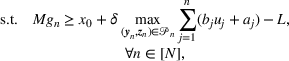
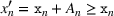
Consider a production system subject to production‐induced degradation and periodic condition monitoring. The system has an initial degradation level At the beginning of period If the system fails during period 


The second assumption above is for tractability in a discrete‐time setting. In practice, δ is typically small due to advances in the IoT technology, making it reasonable to impose the assumption.


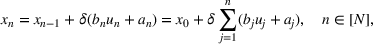
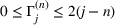
At period 


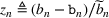
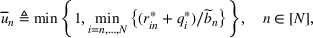
We now quantify the uncertainty of 


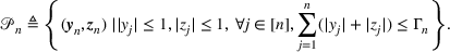


Under the above formulation, we aim to determine the optimal replacement time 


STATIC ROBUST OPTIMIZATION PROBLEM
This section confines to a linear relation between the production and degradation rate, that is, 


Robust counterpart
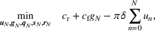
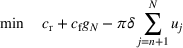
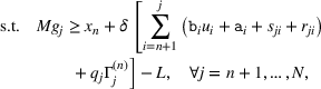
We consider a fixed 


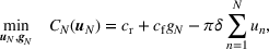


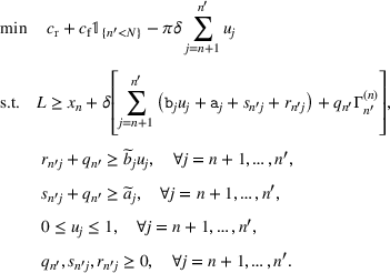
where Problem (3a)–(3e) has the following robust counterpart:


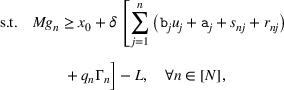


Problem (4a)–(4h) is a mixed integer program that can be solved by off‐the‐shelf solvers. We can further strengthen the integer programming formulation based on the following proposition.


The proposition is intuitive in the sense that the optimal 


The robust counterpart formulated in (4a)–(4h) introduces auxiliary decision variables 


Interestingly, the equivalence revealed above is closely related to the two heuristic policies in uit het Broek et al. (2020). Both heuristics simplify the problem by assuming the degradation evolves deterministically with nominal parameters The first heuristic uses the current degradation level The second heuristic modifies the current degradation level 


Basically, the first heuristic directly decreases the production rate by an amount of α1, which resembles the (smaller) modified upper bound 


Optimal time to replacement
The robust counterpart in Section 3.1 is derived for a fixed number of periods The nominal and the maximum deviation parameters are constant over 


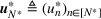
The optimal production rates 


Assumption 1 requires constant nominal values and maximum deviations during the entire planning horizon. The assumption is commonly adopted in maintenance optimization (Chen & Ye, 2018; uit het Broek et al., 2020) and mild when the degradation process has stationary increments under a fixed production rate, which is reasonable for degradation resulting from wear, for example, filters in a waterworks and car tires (Sun et al., 2020). When the degradation process is nonlinear, taking the logarithm of the degradation data often yields a linear path, for example, rolling bearings studied in Elwany et al. (2011). Assumption 2 requires positive (negative) optimal revenue (cost). This assumption holds for reasonable parameter settings; otherwise, the optimal strategy is simply choosing to halt production. Based on Assumptions 1 and 2, we can derive the following results. Under Assumptions 1 and 2, the optimal solution to Problem (4a)–(4h) satisfies 


Since Under Assumptions 1 and 2, the optimal 
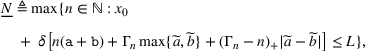


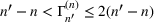
Proposition 2 yields a range 


PRODUCTION CONTROL IN A DYNAMIC ENVIRONMENT
We continue with the linear production–degradation with 


Reoptimization problem in a rolling horizon
A common approach for the optimization problem in a dynamic environment is to use reoptimization whenever new information, which in our case is the newly inspected degradation level, becomes available. After the in situ degradation measurement 


Theoretically, this reoptimization method is a type of static policy in multistage robust optimization problems, which often have good performance in practice (Delage & Iancu, 2015). Similar to Bertsimas and Thiele (2006) and Mamani et al. (2017), the main purpose of our model formulation in (3) is to derive closed‐form solutions that can be easily understood by practitioners. Alternative methods such as affinely adjustable robust optimization and distributionally robust optimization (e.g., Jackson et al., 2019; He et al., 2020) may not admit such closed‐form solutions, which hinders the real‐time implementation of the model for IoT‐enabled production systems.
To reoptimize our production planning problem, the budget of uncertainty at every period needs to be updated. Let 


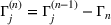


After updating 


In the same spirit as Problem (4a)–(4h), Problem (9) is a mixed‐integer linear program, which is generally time‐consuming to solve. Nevertheless, the next section derives some structural properties to this reoptimization problem, based on which closed‐form solutions are available. This feature makes the implementation of our model as easy as the heuristics in uit het Broek et al. (2020).
Structural properties
Solving (9) directly is generally hard. Nevertheless, we have At time 


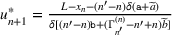
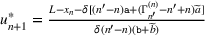
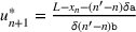
By convention, we set Consider period If If If If 


The key to prove Theorem 2 is to construct a pair of primal‐dual feasible solutions to Problem (10) and show their optimality by strong duality. This construction is largely enabled by Assumption 1. If we can find similar stationary assumptions for other systems, our analysis may also be useful to derive closed‐form solutions for the corresponding control problem. When parameter uncertainty is neglected, that is, 


Recall that our model reveals a relationship between our robust optimization problem and the heuristics proposed in uit het Broek et al. (2020). Specifically, 

NONLINEAR PRODUCTION–DEGRADATION RELATIONS
Robust counterpart
We consider a general η in (1). With this production–degradation relation, the static production planning problem is the same as Problem (3a)–(3e), except that Constraint (3b) is replaced with


The variables 


Based on Corollary EC.2, we follow the same procedure as in Sections 3 and 4 to derive the optimal solution for the dynamic production planning problem under Assumptions 1 and 2. We first solve Problem (EC.11) at time 0 for any fixed 


Convex production–degradation relation
Directly solving the robust counterpart is time‐consuming due to the integer decision variables 


Lemma EC.1 also reveals a structural property of the optimal solution to each convex program corresponding to the robust counterpart: for the optimal production plan, if the system does not produce at its maximum or minimum rate during some periods, then these production rates are equal. A similar result is obtained in uit het Broek et al. (2020, Lemma 2) when the degradation is deterministic. Under parameter uncertainty, our proof to Lemma EC.1 is significantly more complex due to the introduction of auxiliary variables 


Based on Theorem EC.1, one can readily solve the static planning problem in (EC.11) for every fixed 


Next, we fix 


Concave production–degradation relation
Similar to the previous cases, we first use (5) to eliminate the integer decision variables 


Specifically, we confine to 


Motivated by the structural properties of the optimal solution when Under Assumption 1, if 


When 


Statement (i) in Proposition 3 suggests that adding (13a), (13b), and (14) to Problem (EC.13) does not affect its optimal solution when 


We next optimize Under Assumption 1, let 


Based on Theorem 3, we can readily compute 
In practice, we can further input our approximately optimal solution as an initial solution of an interior point algorithm for a warm start, which can possibly find a better production plan with the cost of a longer computational time. Nevertheless, our numerical experiments in Section 6.3 show that the improvement brought by this strategy is insignificant. This shows that the approximately optimal production plan obtained by our algorithm has performed sufficiently well.
APPLICATIONS TO EXTRUDER PRODUCTION
We apply the proposed model to control the production rate of an extruder system, and a graphical illustration of this system is displayed in Figure 1. An extruder produces bottle caps by using a rotating screw to move the melted plastic raw material through a cylinder. Due to wear of the screw, the melted material may leak within the cylinder, and a thermal resistor is then activated for cooling. Hence, we use the mean daily usage frequency of the thermal resistor as a surrogate degradation signal for the screw wear. Section 6.1 analyzes a real‐world extruder degradation dataset, based on which we determine our simulation setting. Section 6.2 uses simulation to compare the performance of our robust model with several existing control methods for the convex production–degradation relation. Section 6.3 further assesses the performance of our model for the concave production–degradation relation. All optimization algorithms are implemented in Python, and all computational times are obtained from a computer with an Intel Core i7 CPU 2.2 GHz processor.
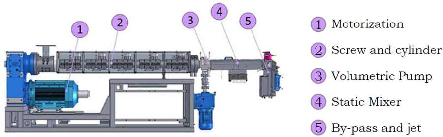
A graphical illustration of the extruder production system in this study. The screw and cylinder are subject to the degradation‐induced failure.
Data analysis
We collect degradation data of an extruder in an Italian factory from the commission date, that is, July 2017 to July 2019. During the study period, the rotational speed 


We adopt two popular degradation models to fit the data 

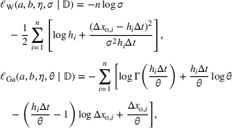
where 


Distributions of the degradation increment at a period under different stochastic process models.


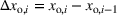
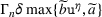
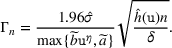
We can use the asymptotic normality results in Appendix A.15 to determine the parameter values in the proposed robust model. We first identify a “working degradation model,” for example, either a Wiener or gamma process, and obtain MLEs of its parameters. Here, we demonstrate using the Wiener process as the working model. The procedure is almost the same for the gamma process. In the robust model, we set 


Experiments on convex production–degradation relations
We first assess the performance of the proposed robust model under convex production–degradation relations. In the simulation, we set the workload adjustment interval as the proposed robust model with parameters determined as in Section 6.1 (referenced as “RO”) using the Wiener process as the working model; the MDP using the correctly specified degradation model (referenced as “MDP”); the MDP using a the deterministic degradation process (referenced as “Deterministic”).


Using the above setting, we consider two scenarios based on the data‐fitting results above. In the first scenario, we use the stationary Wiener process with parameter 


For each of the two settings above, we replicate the simulation 1000 times. Table 2 summarizes the computational time to solve the static planning problem at time 0 for all control methods by averaging over the 1000 replications. As with Bertsimas and Thiele (2006) and Mamani et al. (2017), we then assess the performance of each control method by examining the mean, upper semivariance (USV), and 
Computational times for optimization of the replacement time and static production planning.
Relative performances between robust and benchmark solutions under different degradation models.


Abbreviations: Deterministic, the deterministic degradation process; MDP, the MDP using the correctly specified degradation model; MDP‐MIS, the MDP using a misspecified degradation model; USV, upper semivariance.
The above simulation uses 


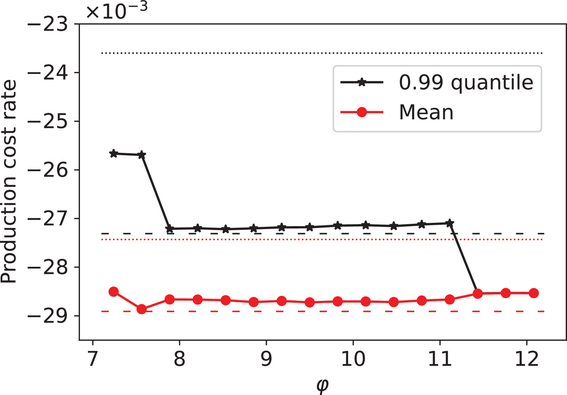
Sensitivity analysis on φ when the actual degradation is the gamma process. Dotted and dash horizontal lines indicate the performance measures obtained from the MDP solution with and without model misspecification, respectively. Red and black separately indicate the empirical mean and 0.99 quantile.
Historical data to determine 


Experiments on concave production–degradation relations
Section 5.3 proposes an algorithm to approximately solve Problem (EC.13) under concave production–degradation relations. We compare the performance of the approximately optimal robust production plan with the MDPs with and without model misspecification. For simplicity, we assume that the actual degradation follows a gamma process; the parameter values used in Section 6.2 are adopted here, except 
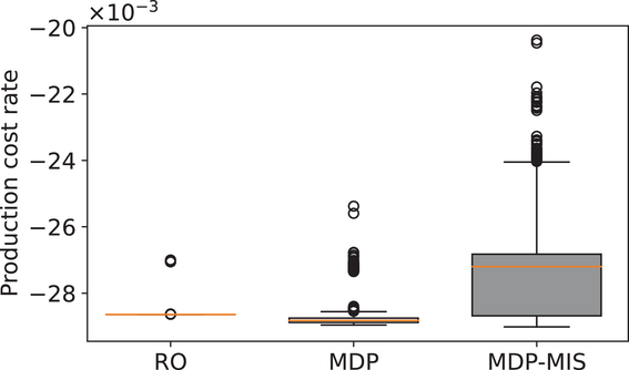
The box plot of the production cost rates obtained from 1000 simulation replications under our robust model and the MDPs with and without model misspecification. MDP, the MDP using the correctly specified degradation model; MDP‐MIS, the MDP using a misspecified degradation model.
Finally, we compare the proposed algorithm in Section 5.3 with the state‐of‐the‐art interior point algorithm. Based on the simulation setting above, we generate a problem instance through randomly sampling the parameter values for the robust model: 


Summary statistics of relative differences (in %) between our algorithm and the interior point algorithm.


Sensitivity analysis
This section further examines the sensitivity of the optimization result with respect to changes in model parameters. We set the gamma process as the actual degradation model as in Section 6.3. For each parameter, we vary the value from 25% to twice of its base value in Sections 6.1 and 6.2 and keep other parameters unchanged. We determine 
Figure 4 compares the long‐run revenue rates (obtained by 1000 simulation replications) under our model and the benchmarks when the cost parameters π, 
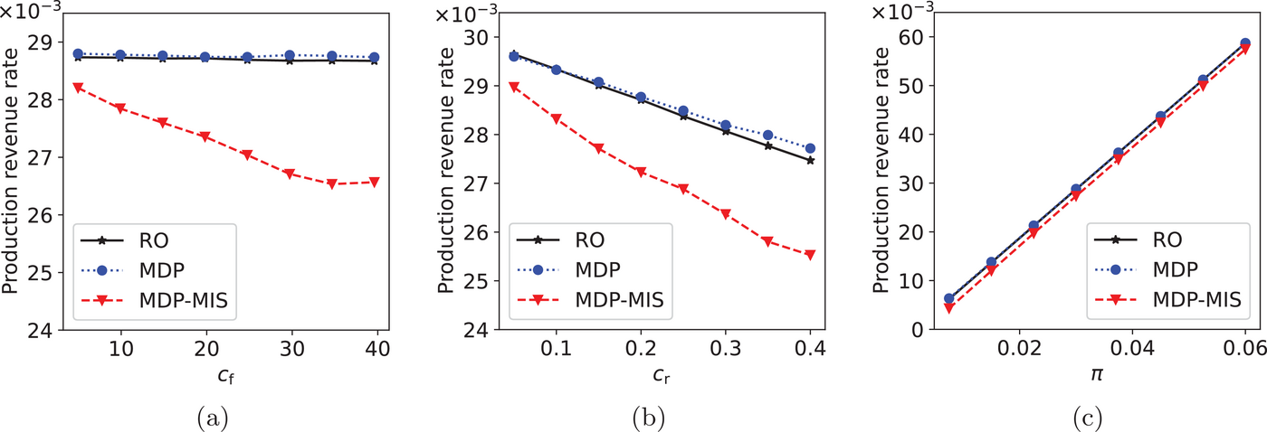
The long‐run production revenues of the robust model and the MDPs with and without model misspecification (obtained from 1000 simulation replications) under different cost parameters. MDP, the MDP using the correctly specified degradation model; MDP‐MIS, the MDP using a misspecified degradation model.
Figure 5 compares the long‐run revenue rates (obtained by 1000 simulation replications) under the robust model and benchmarks when the degradation parameters 
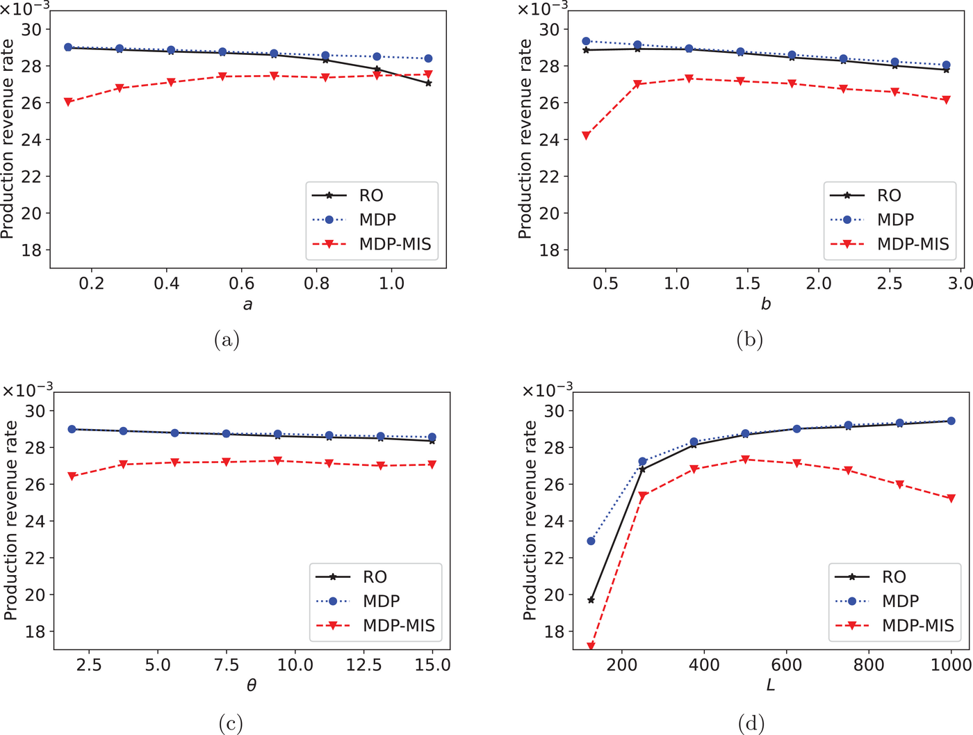
The long‐run production revenues of the robust model and the MDPs with and without model misspecification (obtained from 1000 simulation replications) under different degradation parameters. MDP, the MDP using the correctly specified degradation model; MDP‐MIS, the MDP using a misspecified degradation model.
CONCLUSION
This study develops a robust optimization framework for the optimal production and maintenance control problem for both linear and nonlinear production–degradation relations. The framework circumvents the difficulty of predetermining a stochastic degradation model for optimization. As seen in Section 6, the parameters for the proposed model can be easily determined based on historical degradation data. Based on the derived structural properties, we obtain closed‐form solutions to the optimal (in the case of linear or convex production–degradation relations) or approximately optimal (in the case of concave production–degradation relations) dynamic production rates. Our approximate algorithm for concave production–degradation relations showcases how to use structural results under the deterministic degradation setting to solve nonconvex optimization problems. Both the closed‐form solution and the approximate algorithm ensure real‐time implementation of the proposed model. This appealing feature could enable us to adopt a small enough interinspection interval δ for real‐time control of an IoT‐enabled production system. Moreover, our model lends theoretical support to the heuristics proposed in uit het Broek et al. (2020) from robust optimization. Finally, the application of the extruder example has shown that the proposed model is robust against model misspecification, whereas the optimal cost rate produced from MDP can be 20% higher than the robust solution. The USV of the cost rates obtained from the robust model is also shown to be remarkably smaller than the MDP solutions.
Several topics could be further investigated in the future. First, we determine all model parameters before optimization. In the future, we would investigate the possibility of integrating robust optimization and learning of uncertain parameters (e.g., Lim et al., 2012) for our problem whenever a new degradation level is revealed at a decision epoch. Second, this study estimates the nominal parameters by a working degradation model as implemented in Section 6. We would further investigate the joint estimation and robustness optimization (Zhu et al., 2022) for the condition‐based production planning problem. Last, we could integrate stochastic (multiperiod) demands into the proposed model, so our production plan can be dynamically adjusted to the realized demands over time. The coordination among multiple production systems can also be considered in the presence of stochastic production demands.
Footnotes
ACKNOWLEDGMENTS
The authors would like to thank the editor, a senior editor, and two anonymous referees for their valuable comments and constructive suggestions, which have led to a significant improvement in the quality and presentation of this work. This work was supported in part by the National Science Foundation of China (72071071, 72101145, 72221001), the Singapore MOE AcRF Tier 2 Grant (A‐8001052‐00‐00), and the Shanghai Pujiang Program (21PJC071).