Sage Journals: Discover world-class research

Abstract

We study inventory control with volume flexibility: A firm can replenish using period‐dependent base capacity at regular sourcing costs and access additional supply at a premium. The optimal replenishment policy is characterized by two period‐dependent base‐stock levels but determining their values is not trivial, especially for nonstationary and correlated demand. We propose the Lookahead Peak‐Shaving policy that anticipates and peak shaves orders from future peak‐demand periods to the current period, thereby matching capacity and demand. Peak shaving anticipates future order peaks and partially shifts them forward. This contrasts with conventional smoothing, which recovers the inventory deficit resulting from demand peaks by increasing later orders. Our contribution is threefold. First, we use a novel iterative approach to prove the robust optimality of the Lookahead Peak‐Shaving policy. Second, we provide explicit expressions of the period‐dependent base‐stock levels and analyze the amount of peak shaving. Finally, we demonstrate how our policy outperforms other heuristics in stochastic systems. Most cost savings occur when demand is nonstationary and negatively correlated, and base capacities fluctuate around the mean demand. Our insights apply to several practical settings, including production systems with overtime, sourcing from multiple capacitated suppliers, or transportation planning with a spot market. Applying our model to data from a manufacturer reduces inventory and sourcing costs by 6.7%, compared to the manufacturer's policy without peak shaving.

Keywords

flexibility inventory peak‐shaving robust optimization

INTRODUCTION

Today's logistics environment is characterized by an ongoing shortage of truck drivers (Bhattacharjee et al., 2021), disrupted supply chains in the wake of the pandemic (Berger, 2021), and rising oil prices (Krauss, 2022). Shipping rates for 2022 surged by 20%–100% compared to the year before (Tyagi et al., 2021), forcing manufacturers to make better use of their “base capacity”.

We worked with a manufacturer in the fast‐moving consumer goods industry whose daily replenishments from its factory to distribution centers are characterized by volume flexibility: a third‐party carrier offers guaranteed shipment capacity at a pre‐negotiated contract rate, but above this base capacity, the manufacturer must resort to the transportation spot market. Under the current conditions, the rate premium can easily double the base rate.

The option to source above the current base capacity by paying a premium, referred to as “volume flexibility,” introduces the following trade‐offs. When inventories in the warehouses are low, the manufacturer must decide whether using the more expensive, premium supply is beneficial or whether replenishment can be postponed to later low‐demand periods and supplied at regular rates. Vice versa, when the manufacturer faces forecasts with demand peaks, volume flexibility allows anticipatory ordering at base cost. This lookahead peak shaving has the benefit of avoiding the premium that must be traded off against the resulting increased inventory‐related costs.

Our problem can be modeled as a single‐sourcing inventory system with backlogging. Order quantities are constrained by a weak capacity limit with the flexibility to source above the base capacity at a premium (see Figure 1a). Porteus (1990) shows that under the resulting piece‐wise linear cost structure, a generalized base‐stock policy, characterized by an additional base‐stock level per price segment, minimizes the expected sourcing and inventory costs per period. Under two price segments, the generalized base‐stock policy first places a base order to raise the inventory position to the high base‐stock level. If that quantity exceeds the base capacity, at most the base capacity is ordered (see Figure 1b, green area). After this base order, if the adjusted inventory position is still below the low base‐stock level, additional units are ordered at the premium cost to raise the inventory position to the low base‐stock level (see Figure 1b, blue area).

FIGURE 1

The left panel visualizes our modeling of volume flexibility using a piece‐wise linear sourcing cost in which the first

k_{t}

units incur the pre‐negotiated unit cost c while units beyond

k_{t}

incur an additional premium

c_{p}

. The right panel shows the optimal policy: The order quantity can (I) exceed, (II) equal or (III) be below the base capacity

k_{t}

Unfortunately, there are currently no closed‐form expressions for the optimal base‐stock levels in a stochastic setting that aims to minimize expected costs. One must resort to numerical approaches such as dynamic programming (Lu & Song, 2014; Martínez‐de Albéniz & Simchi‐Levi, 2005). The latter requires discretization of the demand distribution and quickly becomes computationally expensive, especially when demand is nonstationary or correlated. Multivariate comparative statics are needed to understand the interaction among parameters, which is cumbersome for numerical approaches. The nonexistence of closed‐form solutions also hampers implementation in practice. As such, we have seen our manufacturer resorting to simplifying, suboptimal heuristics to set base‐stock levels. This may substantially increase costs, as we also observe in our numerical experiments. We believe this practice may also exist at other companies facing the same problem. They may benefit from simple formulae for the optimal policy. This paper proposes such formulae by utilizing robust optimization.

We show the robust optimality of the Lookahead Peak‐Shaving policy that anticipates or peak shaves orders from future peak‐demand periods to the current period, thereby matching capacity and demand. The Lookahead Peak‐Shaving policy, visualized in Figure 2, is intuitive and works as follows: (a) compute future order quantities assuming an uncapacitated system; (b) working backward from the most future period in the planning horizon, recursively allocate all units that exceed the base capacity in future periods to the closest preceding periods with spare base capacity, except for the current period to quantify the shifting need. This is the total aggregate remaining units above the base capacity in future periods within the planning horizon. It is the amount we would want to shift to the current period if ample capacity were available in the current period; and finally (c) peak shave the remaining units above capacity to the current period until either all units are shifted or the current period's spare capacity is fully used. We refer to the actual amount of units that can be shifted to the current period as the peak‐shaved quantity. Peak shaving differs from conventional smoothing in that it anticipates future order peaks and partially shifts them forward. Conventional smoothing recovers the inventory deficit from demand peaks by increasing later orders.

FIGURE 2

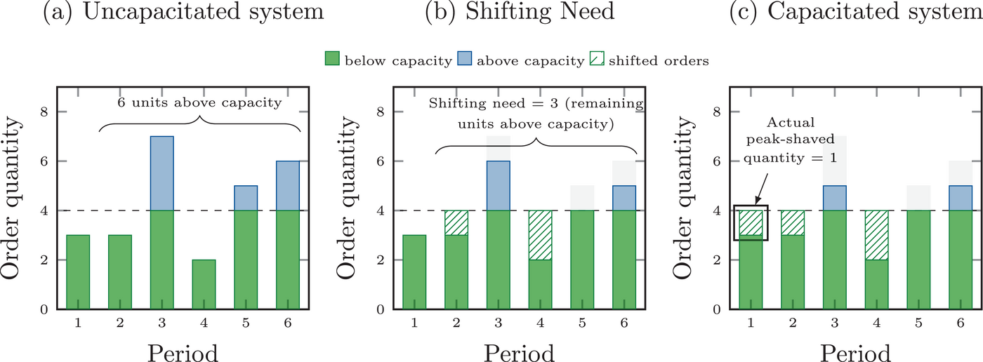
The Lookahead Peak‐Shaving policy: (a) computes order quantities assuming no capacities; (b) determines the shifting need, that is, the desired amount of units to shift to the current period; and (c) peak shaves orders from future capacitated periods to the current period, hereby reducing future premium costs at the expense of increasing the inventory mismatch costs.

The deterministic nature of robust optimization allows capturing the base‐stock levels in a closed form based on the worst‐case demand realizations. The explicit expression of the peak‐shaved quantity yields insight into how and when peak shaving results in filling up the base capacity, thereby reducing future premium costs at the expense of increased inventory mismatch costs. The applicability and effectiveness of our policy are supported by comprehensive numerical analyses and its application using data from our manufacturer. We compare our robustly optimal approach against two heuristic replenishment policies, of which the manufacturer currently adopts one. The numerical experiment shows that our policy performs well, especially when demand is nonstationary, negatively correlated, and when capacity fluctuates. This performance improvement is not only in terms of worst‐case but also in terms of the conventional “expected cost” criterion. We also demonstrate how the manufacturer may use his forecast and related forecast errors to compute the worst‐case realizations needed to determine the base‐stock levels. The application of our Lookahead Peak‐shaving policy on 869 products of the manufacturer results in 6.7% cost savings.

In sum, our contribution is threefold: (1) We prove the robust optimality of the Lookahead Peak‐Shaving policy with a novel proof technique based on the Simplex algorithm; (2) our robustly optimal policy also yields excellent performance in terms of expected cost, especially when demand is nonstationary and negatively correlated, and when capacities fluctuate around the mean demand; (3) our explicit expressions are intuitive, easy to apply in practice and allow multivariate “what‐if” analyses, yielding insights into how peak shaving pro‐actively matches capacity and demand. Our model easily extends to other settings where flexible supply is prevalent such as companies with a dedicated workforce but the option to pay for overtime or part‐time labor or contracts may be used to source from a preferred supplier up to a predefined level, but with the option to resort to back‐up suppliers at a higher cost.

RELATED LITERATURE

We contribute to the stochastic inventory control literature by building on methods and techniques from the field of robust optimization. When sourcing costs are linear in the ordered volume, inventory mismatch costs are convex and unmet demand may be backlogged, Karlin and Scarf (1958a) prove that a base‐stock policy minimizes expected costs. Karlin (1958) extends the linear sourcing cost assumption to any convex function and shows that the latter makes the optimal base‐stock level dependent on the inventory levels before order placement. Low inventory levels induce lower base‐stock levels: it is better to partially postpone orders and incur an additional inventory mismatch than ordering now at a higher unit sourcing cost. Porteus (1990, p. 662) refers to this policy as a generalized base‐stock policy. Porteus (1990) shows that there are a finite number of base‐stock levels if the sourcing cost is piece‐wise linear and convex. In particular, when the sourcing cost has two linear segments, the optimal policy is defined by two base‐stocks that determine when the capacity is deceeded, exactly used, or exceeded (as visualized in Figure 1b). We will show that the robustly optimal policy exhibits the same policy structure.

While the optimal policy structure is known in a conventional stochastic setting, the optimal base‐stock levels are not. Lu and Song (2014) use dynamic programming to obtain the optimal order quantities. This computational approach, however, does not scale extremely well although Martínez‐de Albéniz and Simchi‐Levi (2005) demonstrate how to reduce the computational effort by limiting the search space. Yet, both articles assume perfect knowledge about the demand distribution, an assumption we will relax. Henig et al. (1997) investigate a similar model in which a contracted capacity of k units is purchased in advance, such that the first k units can be sourced at no cost. The piece‐wise linear sourcing cost function is identical to our system. They numerically obtain the optimal base‐stock levels by enumerating over all base‐stock level combinations, using the underlying Markov chain. Gijsbrechts et al. (2022) investigate a dual sourcing model in which the fast source has a piece‐wise linear sourcing cost function. They find explicit expressions for the fast base‐stock levels when a second slow source with linear sourcing costs is available. Yet, their results do not hold for single sourcing.

We employ robust optimization and refer to Ben‐Tal et al. (2009) for a good introduction. Robust optimization provides an alternative to stochastic optimization by minimizing the worst‐case cost, that is, the maximum possible cost, rather than minimizing the expected cost. Min–max approaches have been used since the early days of inventory control. Karlin and Scarf (1958b), for instance, minimizes the expected cost for all demand distributions with the same mean and standard deviation. Within linear programming, Soyster (1973) introduces interval uncertainty implying the uncertain parameters (in our study the demand distribution) are constrained to lie within a specific interval around their nominal (i.e., expected) values while the worst case scenario is minimized. A weakness of using interval uncertainty is that, by definition, we always buffer against the most extreme cases. For instance, while demand may deviate significantly within periods, it is often unlikely that the worst‐case demand appears every period.

The demand data of the companies we have worked with all contain signification fluctuations on a daily basis. Yet, the monthly cumulative demand is prone to less variability. This conservative nature of interval uncertainty hampered widespread adoption of robust optimization in inventory control, both in theory and in practice. That is, until Bertsimas and Sim (2004) pioneered the use of “budgets of uncertainty” to reduce the level of conservatism. In addition to uncertainty intervals around the uncertain variables, they restrict the cumulative deviation from the nominal values of all uncertain variables to be within a budget. Their approach is intuitive: the uncertainty may be large in specific periods but the cumulative deviation typically reduces as the planning horizon increases. For instance, we may have poor daily forecasts on consumer demand but the monthly relative forecast error is typically smaller—as we also observe in our data set. This opened the door toward many follow‐up papers within inventory control. Bertsimas and Thiele (2006) demonstrate how to apply the method of Bertsimas and Sim (2004) on several classic inventory problems, such as single sourcing with, and without, a fixed set‐up cost, systems with hard capacity constraints on the orders and inventory levels, and networked multi‐echelon systems. Interestingly, they show that the optimal robust structure is often identical to its stochastic counterpart. These results are powerful as they demonstrate that robust formulations may perform well in stochastic settings when the uncertainty sets are chosen well. In other words, when the policy structure is alike, the robust policy parameters may be tuned in such a way that the resulting robust policy and its parameters match the optimal stochastic policy parameters. As such, without requiring the exact demand distribution, the robust policy is capable of achieving the same cost performance as the stochastically optimal policy when evaluated on the expected cost performance measure. This is an appealing feature when the knowledge on the stochastic distribution is sparse. We build further on the aforementioned works by tackling an inventory system in which the sourcing costs are piece‐wise linear and convex while leveraging a specific parameterization of the worst‐case uncertainty realizations set to derive closed‐form expressions of the policy parameters. Moreover, we demonstrate the resulting cost savings when we apply our model to a real data set.

Determining the budgets of uncertainty forms an important aspect of robust optimization. In other words: “How do we trade‐off expected cost performance in a stochastic setting versus conservatism?” A fundamental method was coined by Bandi and Bertsimas (2012), proposing the use of the central limit theorem (CLT) to constrain the periodic and cumulative uncertainty by the period means and standard deviations. Mamani et al. (2017) use the same CLT approach to define their uncertainty sets with respect to the period means and standard deviations. In doing so, they provide closed‐form expressions of the robustly optimal policy parameters in classic single sourcing inventory management settings with linear transportation costs that only rely on the first two moments of the demand distribution. We employ the same uncertainty sets as Mamani et al. (2017) but apply them to the system with piece‐wise linear sourcing costs. For a detailed overview of robust optimization including piecewise linear functions, we refer to Gorissen and Den Hertog (2013) and Ardestani‐Jaafari and Delage (2016). Our problem is part of their class of problems. While Ardestani‐Jaafari and Delage (2016) consider the generic robust optimization problem for piecewise linear functions, we are able to analytically solve for the optimal policy of the specific robust optimization problem of volume flexibility. Wagner (2018) extends the results of Mamani et al. (2017) to continuous review and provides useful insights on how to implement robust order quantities in a dynamic rolling horizon setting. Employing robust optimization does not only provide a tractable way to solve large‐scale problems, it also allows for a deeper analysis of policy structure and related policy parameters. Sun and Van Mieghem (2019), for instance, introduce, and prove robust optimality of capped dual index policies in dual sourcing settings with nonconsecutive lead times; settings where little is known about the optimal stochastic policy despite some asymptotic results (Xin & Goldberg, 2018). Moreover, they numerically show their policy performs exceptionally well on a diverse set of stochastic settings.

We contribute to the aforementioned streams by determining the robustly optimal policy structure when sourcing costs are piece‐wise linear and convex. Moreover, we manage to provide closed‐form expressions of the optimal parameters in settings that we believe to be widely applicable in practice. As such we propose a tractable model that provides insight in how orders should be placed to benefit from the contracted supply capacity.

MODEL OF CAPACITATED SOURCING WITH VOLUME FLEXIBILITY

We model the transportation sourcing problem with volume flexibility as a periodically reviewed inventory system with backlogging and piece‐wise linear, convex sourcing costs. The lead time is zero to avoid notational clutter but our results hold for longer lead times. We will next outline the stochastic formulation of the problem together with the stochastically optimal policy and subsequently introduce the robust formulation of the problem. For the remainder of the paper, we use the following notational conventions: vectors are denoted in bold; summations

\sum_{i = a}^{b} x_{i} = 0

b < a

;

N_{a}^{b}

denotes the set

{a, a + 1, \dots, b}

; the slack of

a \cdot x \leq b

{(b - a \cdot x)}^{+}

. If the slack is zero, we say the inequality is binding; and

{(\cdot)}^{+}

and

{(\cdot)}^{-}

denote the positive and negative part operator, respectively. The proofs of our lemmas, theorems, and corollaries are relegated to Appendix A in the Supporting Information.

Stochastic model

The demand

d_{t}

in each period t is distributed with mean

μ_{t}

and standard deviation

σ_{t}

that are assumed to be known data. Both moments can be period‐dependent and we allow for correlation between periods. Given lead time zero there are no outstanding orders and we have the following sequence of events. Each period t, we first observe the net ending inventory of the previous period

x_{t - 1}

. Based on the ending inventory, the order quantity

q_{t}

is determined. The order arrives immediately before observing and satisfying the demand

d_{t}

. Hence, the net inventory at the end of a period evolves as follows:

\begin{matrix} x_{t} = x_{t - 1} + q_{t} - d_{t} . \end{matrix}

1Costs are computed at the end of each period. Any unit left at the end of the period incurs a holding costs h, while any unit backlogged incurs a backorder penalty b. Each unit of the ordered quantity

q_{t}

incurs a unit sourcing cost of c. Capacity is flexible: orders exceeding the base capacity incur an additional sourcing premium of

c_{p}

per unit. The sourcing costs hence consist of two line segments with slopes c and

c + c_{p}

as depicted in Figure 1a. The weak capacity limit

k_{t}

can vary per period. The cost in period t, denoted by

C_{t}

, is thus given by:

C_{t} (x_{t}, q_{t}) = h x_{t}^{+} - b x_{t}^{-} + c q_{t} + c_{p} {(q_{t} - k_{t})}^{+} .

A feasible policy, π, consists of a sequence of mappings

f_{t}^{π} : R \mapsto R, t \geq 1

. That is, based on the net ending inventory position

x_{t - 1}

we aim to find the order quantity

q_{t} = f_{t}^{π} (x_{t - 1})

. Let

C_{t}^{π}

denote the cost of policy π in period t. The long‐run average cost of policy π is given by:

\begin{matrix} C (π) ≜ \lim_{T \to \infty} \frac{1}{T} \sum_{t = 1}^{T} E (C_{t}^{π}) . \end{matrix}

Let Π denote the set of all feasible ordering policies. The objective for stochastic inventory management with volume flexibility is to find a policy

π \in Π

that minimizes the long‐run average cost:

\begin{matrix} C^{OPT} ≜ inf_{π \in Π} C (π) . \end{matrix}

[Stochastic objective]

The structure of the optimal policy

π^{*}

is known (Porteus, 1990), characterized by two base‐stock levels

S_{t}^{2} \leq S_{t}^{1}

, as visualized in Figure 1b. It works as follows: Place a base order of at most

k_{t}

units to raise the inventory level before ordering,

x_{t - 1}

, up to

S_{t}^{1}

, if that is possible. If, after this initial order, the adjusted inventory position is still below

S_{t}^{2}

, order additional units at an overtime premium to reach

S_{t}^{2}

. This introduces a region of inaction,

x_{t - 1} \in [S_{t}^{2} - k_{t}, S_{t}^{1} - k_{t}]

, in which exactly

k_{t}

units are ordered. The region of inaction causes the orders to be nondemand replacing and effectively levels the order quantities: it incurs a higher inventory mismatch cost to avoid the price premium of the supply above

k_{t}

. The optimal order quantity in period t satisfies:

\begin{matrix} q_{t}^{★} (x_{t - 1}) = \{\begin{matrix} {(S_{t}^{2} - x_{t - 1})}^{+} & if x_{t - 1} < S_{t}^{2} - k_{t}, \\ k_{t} & if S_{t}^{2} - k_{t} \leq x_{t - 1} < S_{t}^{1} - k_{t}, \\ {(S_{t}^{1} - x_{t - 1})}^{+} & if S_{t}^{1} - k_{t} \leq x_{t - 1} . \end{matrix} \end{matrix}

To the best of our knowledge, no closed‐form expressions of the period‐dependent policy parameters

S_{t}^{1}

and

S_{t}^{2}

exist. In the following section, we show how to leverage a robust rolling horizon formulation to provide insights in how to efficiently set the base‐stock levels. In contrast to stochastic programming, it only requires the first two moments of the demand distribution rather than the full distribution. Moreover, it is more flexible in comparison to heuristics used in practice to include past and future information about demand and capacity.

Robust model

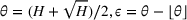
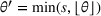
We adopt a robust rolling horizon formulation similar to Sun and Van Mieghem (2019) that works as follows. In each period t, we look ahead and optimize order quantities over a fixed planning horizon of length H. We determine the robustly optimal ordering vector

q_{t}

q_{t}, \dots, q_{t + H - 1}

) that minimizes the worst‐case cost over all possible demand realizations

d_{t}

d_{t}, \dots, d_{t + H - 1}) \in Ω_{t}

. The uncertainty set

Ω_{t}

denotes the set of all feasible demand realizations within the planning horizon

N_{t}^{t + H - 1}

. We denote the minimum and maximum cumulative demand from period t to period n by

{\underset{̲}{D}}_{n} = \min_{(d_{t}, \dots, d_{n}) \in Ω_{t}} \sum_{i = t}^{n} d_{i} and {\bar{D}}_{n} = \max_{(d_{t}, \dots, d_{n}) \in Ω_{t}} \sum_{i = t}^{n} d_{i},

3respectively.

In each period t, we optimize the quantity vector

q_{t}

by looking ahead over the planning horizon

[t, t + H - 1]

. Yet, while we optimize for the full quantity vector

q_{t}

, we only implement its first element

q_{t}

in period t. We then observe demand

d_{t}

, proceed to the next period and update the inventory state using inventory balance equation (1). Then we re‐optimize in period

t + 1

the quantity vector

q_{t + 1}

, and repeat this process at infinitum.

The optimization problem we solve in every period is similar to Mamani et al. (2017) but adapted to include a piece‐wise linear sourcing cost: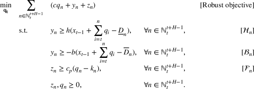

\begin{matrix} \min_{q_{t}} & \sum_{n \in N_{t}^{t + H - 1}} & (c q_{n} + y_{n} + z_{n}) & [Robust objective] \\ s.t. & y_{n} \geq h (x_{t - 1} + \sum_{i = t}^{n} q_{i} - {\underset{̲}{D}}_{n}), & \forall n \in N_{t}^{t + H - 1}, & [H_{n}] \\ y_{n} \geq - b (x_{t - 1} + \sum_{i = t}^{n} q_{i} - {\bar{D}}_{n}), & \forall n \in N_{t}^{t + H - 1}, & [B_{n}] \\ z_{n} \geq c_{p} (q_{n} - k_{n}), & \forall n \in N_{t}^{t + H - 1}, & [F_{n}] \\ z_{n}, q_{n} \geq 0, & \forall n \in N_{t}^{t + H - 1} . \end{matrix}

4The objective function contains for each period

n \in N_{t}^{t + H - 1}

the sourcing costs at the contracted rate (

c q_{n}

), the worst case inventory mismatch cost (

y_{n}

) and the sourcing costs at the premium rate (

z_{n}

). Constraint sets

H_{t} = (H_{t}, \dots, H_{t + H - 1})

and

B_{t} = (B_{t}, \dots, B_{t + H - 1})

bound the cumulative inventory holding/backlog costs, respectively, to their worst case values. The flexibility constraint set

F_{t} = (F_{t}, \dots, F_{t + H - 1})

, finally, enforces the premium rate for orders exceeding the periodic capacity constraint

k_{n}

. The order quantities

q_{n}

are restricted to be nonnegative.

It remains to describe the uncertainty set

Ω_{t}

. We adopt the uncertainty set formulation of Mamani et al. (2017) that bounds the demand per period and the cumulative demand over several periods. This relates to practice in an intuitive way: the one‐period ahead demand forecast may deviate heavily but the aggregate forecast error over several periods tends to be more stable. We refer to Mamani et al. (2017) (Subsection 2.3) for the general description of the uncertainty set and directly introduce the parameterization of the uncertainty set that we will use throughout this study. The parameterization is inspired by the CLT and was introduced by Bandi and Bertsimas (2012). The uncertainty set

Ω_{t}

in period t consists then of two sets of constraints: (1) periodic constraints that bound each period's demand to be be within an interval around the periodic means:

μ_{n} - {\hat{Γ}}_{n} σ_{n} \leq d_{n} \leq μ_{n} + {\hat{Γ}}_{n} σ_{n}

; and (2) cumulative constraints that bound the cumulative demand over multiple periods around the sum of the mean demands:

\sum_{i = t}^{n} μ_{i} - Γ_{n} σ_{t}^{n} \leq \sum_{i = t}^{n} d_{i}, \leq \sum_{i = t}^{n} μ_{i} + Γ_{n} σ_{t}^{n}

. The cumulative bounds use

σ_{t}^{n}

representing the standard deviation of the cumulative demand from period t to period n, which equals

{(e_{n - t + 1}^{'} Σ_{t}^{n} e_{n - t + 1})}^{1 / 2}

, in which

e_{n - t + 1}

is a

1 \times (n - t + 1)

vector of ones,

Σ_{t}^{n}

is the covariance matrix of demands from periods t to n and

e^{'}

denotes the transpose of

e

Note that we adopt a rolling horizon approach and start indexing from period t. Nonetheless, demand realizations before period t may influence demand within the planning horizon when demand is correlated. Each period, we thus update the vector of means

μ_{t} = (μ_{t}, \dots, μ_{t + H - 1})

and the covariance matrix

Σ_{t}^{n}

using the multivariate normal distribution conditioned on the past realizations to ensure the correlation is accounted for. In Section 6, we adopt the latter approach on a numerical example where demand is correlated according to an AR(1) model.

Both sets of bounds

{\hat{Γ}}_{t} = ({\hat{Γ}}_{t}, \dots, {\hat{Γ}}_{t + H - 1})

and

Γ_{t} = (Γ_{t}, \dots, Γ_{t + H - 1})

are tunable parameters that determine the maximum deviation from the (cumulative) mean demand. Even though they are period‐dependent, they may be set equal for each period such that we only have two degrees of freedom to determine the level of conservativeness. Sun and Van Mieghem (2019), for instance, implement the same

{\hat{Γ}}_{n}

and

Γ_{n}

for all

n \in N_{t}^{t + H - 1}

in their robust formulation of the dual sourcing inventory problem. We will show in Subsection 6.1 how keeping the period‐dependent maximum deviations equal for each period also yields an efficient well‐performing heuristic policy in our setting.

The above formulation results in a symmetric uncertainty set:

\begin{matrix} Ω_{t}^{Sym} & = & \{d_{t} = (d_{t}, \dots, d_{t + H - 1}) : - Γ_{n} \leq \sum_{i = t}^{n} \frac{d_{i} - μ_{i}}{σ_{t}^{n}}, \\ \leq & Γ_{n}, μ_{n} - {\hat{Γ}}_{n} σ_{i} \leq d_{n} \leq μ_{n} + {\hat{Γ}}_{n} σ_{n}, \forall n \in N_{t}^{t + H - 1}\} . \end{matrix}

5For the symmetric formulation, we obtain the minimum and maximum cumulative demand for the specific parameterization of the uncertainty set (see Supporting Information of Mamani et al., 2017, eqs. 21 and 22).

\begin{matrix} {\underset{̲}{D}}_{n} = \sum_{i = t}^{n} μ_{i} - Δ d_{n} and {\bar{D}}_{n} = \sum_{i = t}^{n} μ_{i} + Δ d_{n}, \end{matrix}

with

\begin{matrix} Δ d_{n} = \min \{\sum_{i = t}^{n} {\hat{Γ}}_{i} σ_{i}, Γ_{t + H - 1} σ_{t}^{t + H - 1} + \sum_{i = n + 1}^{t + H - 1} {\hat{Γ}}_{i} σ_{i}\} . \end{matrix}

In Appendix A (in the Supporting Information), we also provide the asymetric formulation of the uncertainty set.

SOLUTION OF THE ROBUST MODEL

Solution for the uncapacitated system

We first review some established results in robust sourcing with a linear sourcing cost, from here on denoted as the uncapacitated system, as we rely on these results in our system with capacities. The uncapacitated system is a special case of our formulation by letting

k_{i} \to \infty

for all i, or by letting

c_{p} = 0

, that is, the linear program must be solved (see Equation 4) without the constraint set

F_{t}

. Both Bertsimas and Thiele (2006) and Mamani et al. (2017) show robust optimality of the base‐stock policy in the uncapacitated system. The expression of the worst‐case demand in Mamani et al. (2017), see also Equation (3), allows for a closed‐form expression of the optimal base‐stock level in every period.

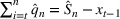
We denote the optimal order quantities that solve the deterministic linear program in the uncapacitated system (Equation 4 without the constraint set

F_{t}

) as

{\hat{q}}_{t}

. They can be obtained by solving the following recursion backward:

\sum_{i = t}^{n} {\hat{q}}_{i} = \{\begin{matrix} {(\frac{b {\bar{D}}_{n} + h {\underset{̲}{D}}_{n}}{b + h} - x_{t - 1})}^{+}, & n \in N_{t}^{T - u + 1} \\ 0, & n \in N_{T - u}^{t + H - 1} \end{matrix}

6with

u b < c \leq (u + 1) b

, where u is the period after which it is cost‐efficient to incur the backlog penalty until the end of the planning horizon, hence nothing is ordered for

i \geq T - u

. This equation is obtained by balancing the worst case holding and worst case backlog costs in each period. In each period

i \leq T - u + 1

, constraints

H_{i}

and

B_{i}

are both binding, otherwise we can either increase or reduce

{\hat{q}}_{i}

to obtain savings.

Equation (6) can thus be formulated using cumulative base‐stock levels: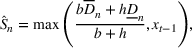

{\hat{S}}_{n} = \max (\frac{b {\bar{D}}_{n} + h {\underset{̲}{D}}_{n}}{b + h}, x_{t - 1}),

7where

x_{t - 1}

denotes the inventory at the start of period t (before ordering). Note that we include the inventory state in the definition of the cumulative base‐stock levels. This simplifies later equations as the base‐stock levels account for high starting inventories. The cumulative order quantity in period n becomes

\sum_{i = t}^{n} {\hat{q}}_{n} = {\hat{S}}_{n} - x_{t - 1}

. Any individual order

{\hat{q}}_{n}

is thus computed by comparing the projected inventory position (i.e., the sum of inventory on hand and order quantities in absence of demand) with the worst‐case future cumulative demands. Interestingly, the optimal order‐up‐to‐level of this robust policy equals a newsvendor solution for the stochastic model as if the cumulative demand were uniformly distributed over the interval [

{\underset{̲}{D}}_{n}, {\bar{D}}_{n}

The rolling horizon optimal order in period 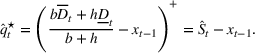t is obtained by solving

{\hat{q}}_{t}^{★} = {(\frac{b {\bar{D}}_{t} + h {\underset{̲}{D}}_{t}}{b + h} - x_{t - 1})}^{+} = {\hat{S}}_{t} - x_{t - 1} .

8Using the parameterizations of the uncertainty set as introduced in Subsection 3.2, the base‐stocks in period t are

\begin{matrix} {\hat{S}}_{t} = \{\begin{matrix} \max (μ_{t} + {\hat{Γ}}_{t} σ_{t} \frac{b - h}{b + h}, x_{t - 1}) & for d_{t} \in Ω_{t}^{Sym} \\ \max (\frac{b}{b + h} (μ_{t} + {\hat{Γ}}_{t} σ_{t}), x_{t - 1}) & for d_{t} \in Ω_{t}^{Asym} \end{matrix} . \end{matrix}

Solution for the capacitated system

We determine the optimal robust order policy and policy parameters for piece‐wise linear and convex sourcing costs starting from the solution of the uncapacitated system described in Subsection 4.1. Note that the robustly optimal order quantities

\hat{q_{t}}

of a system with no capacity limits are a feasible solution to our linear program with

y_{n} = h (x_{t - 1} + \sum_{j = t}^{n} {\hat{q}}_{j} - {\underset{̲}{D}}_{n}) = - b (x_{t - 1} + \sum_{j = t}^{n} {\hat{q}}_{j} - {\bar{D}}_{n})

and

z_{n} = c_{p} {({\hat{q}}_{n} - k_{n})}^{+}

. Earlier, we visualized an example in Figure 2a. Subsequently, we show how this feasible solution, which is optimal in the uncapacitated system, can be improved under a piece‐wise linear sourcing cost by shifting orders between periods to avoid the premium in periods where the orders exceed the base capacity at the expense of increasing the inventory mismatch costs. Clearly, if none of the capacity constraints,

F_{n}

, is tight under feasible ordering quantities,

{\hat{q}}_{n}

, then

{\hat{q}}_{n}

is optimal in a system with volume flexibility too. This is, for instance, the case if all

k_{n}

are sufficiently large. Otherwise, we can improve the feasible

{\hat{q}}_{n}

by advancing or postponing orders as Lemma 1 shows: Lemma 1

When the inventory constraints

H_{i}

and

B_{i}

are tight for all

i \in N_{t}^{t + H - 1}

, advancing (postponing) ω units of

{\hat{q}}_{n}

from period n to period j increases the inventory mismatch by

h ω (n - j)

(

b ω (j - n)

) while reducing the sourcing costs by

c_{p} ω

F_{n}

is tight and

F_{j}

has available slack

k_{j} - {\hat{q}}_{j} > ω

Lemma 1 shows that in the system with piece‐wise linear sourcing costs, the robustly optimal order quantities

\hat{q}

of an uncapacitated system can be improved by shifting orders from capacitated periods to periods that have a capacity slack, if

h < c_{p}

or if

b < c_{p}

. If the premium cost dominates, that is, h and b are smaller than the premium

c_{p}

we must solve the linear program, given in (4), to determine the optimal order quantities. This includes the special case of a hard capacity constraint (

c_{p} \to \infty

) that has been treated in Mamani et al. (2017). They propose using the robust linear order quantities and capping them by the capacity constraint. This approach (for

h, b \leq c_{p}

c_{p} \to \infty

) essentially only postpones orders, while the Lookahead Peak‐Shaving policy (for

h \leq c_{p} \leq b

) only advances orders. Even though we investigate different systems, our work may help to understand why their proposed policy is not optimal in the likely case where

h < b

. In this case, shifting orders to earlier periods is more desirable than shifting orders to later periods. In many practical settings, such as the one we study at our manufacturer, service levels are high such that

b ≫ c_{p}

. As such, for the remainder of the paper, we assume

h < c_{p} < b

. Then, orders from capacitated periods will always be shifted forward to prior uncapacitated periods. When

b < c_{p} < h

, orders will be postponed rather than shifted forward, and all insights remain. When

c_{p} < h < b

orders are never shifted and we recover the uncapacitated system. Henceforth, we thus assume: Assumption 1

The flexibility premium does not exceed the backlog penalty and the holding cost does not exceed the flexibility premium, that is,

h < c_{p} < b

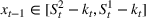
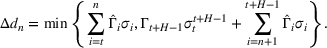
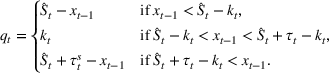
Under Assumption 1, it is only valuable to shift orders forward to avoid the sourcing premium cost. There is a potential need to shift orders from period s to the current period t if the uncapacitated order quantity exceeds the available base capacity. In Figure 2a, for instance, in peak‐demand periods 3, 5, and 6 the uncapacitated orders exceed the available capacity. There is no need to shift orders from a future period s if the uncapacitated order quantity in this period is less than the available base capacity in the same period. This happens in low‐demand periods 2 and 4 in Figure 2a. A future low‐demand period reduces the need to shift orders to the current period as the slack capacity can absorb some or all of the units above base capacity of the later peak‐demand periods. See for instance how periods 2 and 4 absorb some of the units above base capacity of later peak‐demand periods in Figure 2b. We define the shifting need as the remaining amount of units we want to shift to the current period after all future low‐demand periods have absorbed units from later peak‐demand periods. The shifting need is thus visualized by the remaining orders above capacity in Figure 2b. Formally, Definition 1 expresses the shifting need from periods within the lookahead horizon (period

t + 1

to period s) toward period t: Definition 1

Let

{\hat{q}}_{i}

be the optimal order quantities of the uncapacitated system as defined in Equation (6). The shifting need at time t over a lookahead horizon of s periods is defined as

\begin{matrix} τ_{t}^{s} & : = \max_{i \in N_{t + 1}^{t + s}} {(\sum_{j = t + 1}^{i} ({\hat{q}}_{j} - k_{j}))}^{+} . \end{matrix}

We further define the earliest period in which the maximum is attained as

\begin{matrix} M (τ_{t}^{s}) & : = \min \underset{i \in N_{t + 1}^{t + s}}{\arg \max} {(\sum_{j = t + 1}^{i} ({\hat{q}}_{j} - k_{j}))}^{+} . \end{matrix}

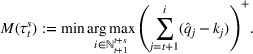
Here, the sum

\sum_{j = t + 1}^{i} ({\hat{q}}_{j} - k_{j})

expresses the total shifting need to shift orders to the current period t from future periods

t + 1

up to period i. If the sum is negative, it implies that there is more capacity slack than sourcing above capacity such that no units need to be shifted to the current period. The sum is positive when the periods

t + 1

i - 1

have insufficient spare capacity to handle the peak demand in i. In this case there is a shifting need from period i to t.

We summarize three observations with respect to the shifting need in Corollary 1: Corollary 1

The shifting need has sensitivities: (a)

\partial τ_{t}^{s} / \partial x_{t - 1} \in {0, - 1}

(b)

\partial τ_{t}^{s} / \partial k_{n} \in {0, - 1} \forall n \in N_{t + 1}^{t + s}

(c)

Δ τ_{t}^{s} / Δ s \geq 0

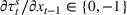
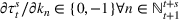
First, the shifting need is indirectly dependent on the starting inventory due to the dependency on the order quantities of the uncapacitated system. If the starting inventory is large, the uncapacitated order quantities are lower, and vice versa. Thus, with more starting inventory, the shifting need decreases (or stays the same, if there was no shifting need). Second, any increase in the capacity of a future capacity leads to a decrease in the shifting need if that period had an impact on the shifting need. Else, the shifting need will stay constant, if there was no shifting need in that period. Third, the shifting need naturally increases (or remains constant) when shifting is considered over a longer horizon s.

Formulating the shifting need with respect to the worst‐case demand realizations, as defined in (3), results in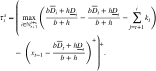

\begin{matrix} τ_{t}^{s} & = (\max_{i \in N_{t + 1}^{t + s}} (\frac{b {\bar{D}}_{i} + h {\underset{̲}{D}}_{i}}{b + h} - \frac{b {\bar{D}}_{t} + h {\underset{̲}{D}}_{t}}{b + h} - \sum_{j = t + 1}^{i} k_{i}) \\ - {(x_{t - 1} - \frac{b {\bar{D}}_{t} + h {\underset{̲}{D}}_{t}}{b + h})}^{+})^{+} . \end{matrix}

10The shifting need consists of two parts: the first part describes the potential shift to period t independent of the starting inventory, the second part reduces the shift by the capacity that becomes available when starting inventory is high and exceeds the base‐stock of period t.

We find that less volume is shifted forward when holding costs increase, but more volume is shifted forward when backlogging and the overtime premium increase. This result is intuitive: when it is more expensive to hold inventory, fewer orders will be shifted forward to avoid future overtime premiums; likewise, if the backlog penalty increases, less orders will be postponed to avoid the overtime premium in the current period. Based on Equation (10), we obtain the sensitivities of the shifting need captured by the following corollary: Corollary 2

The shifting need has sensitivities: (a)

\partial τ_{t}^{s} / \partial h \leq 0

(b)

\partial τ_{t}^{s} / \partial b \geq 0

From Lemma 1, we observe that it is profitable to shift orders as long as we do not shift more than

⌊ c_{p} / h ⌋

periods. Shifting more than

⌊ c_{p} / h ⌋

periods forward is never profitable as the increase in inventory holding cost is no longer offset by the premium incurred by sourcing above capacity in a future period. From now on, we refer to

s = ⌊ c_{p} / h ⌋

as the lookahead horizon. The length of our planning horizon H should exceed the lookahead horizon, denoted by

s = ⌊ c_{p} / h ⌋

, to ensure we capture all cost savings compared to the uncapacitated system. Moreover, we only place orders when the sourcing cost c exceeds the cost of backlogging until the end of the planning horizon. Given that we adopt an infinite rolling horizon approach, we want to avoid the end‐of‐horizon effect where our policy would stop ordering. The length of the planning horizon H should thus also exceed

⌊ c / b ⌋

. Hereafter we thus assume: Assumption 2

The length of the planning horizon satisfies:

H > ⌊ c_{p} / h ⌋

and

H > ⌊ c / b ⌋

We can now formulate the robustly optimal policy for the capacitated system. The robustly optimal policy advances orders from periods with demand peaks to period t, as long as there is spare capacity to source at regular cost c in period t. If there is no slack capacity in period t, the order quantity is identical to the order quantity in the uncapacitated system. We term this policy the Lookahead Peak‐Shaving policy as it looks ahead and shaves the peak of the order quantities in future capacitated periods while increasing the current period's order quantity when there is spare capacity in the current period (see Figure 2). Definition 2

The Lookahead Peak‐Shaving policy over a lookahead horizon of s periods is a generalized base‐stock policy where the lower base‐stock level

{\hat{S}}_{t}

equals the base‐stock level of an uncapacitated system and the upper base‐stock level equals

{\hat{S}}_{t} + τ_{t}^{s}

. The order quantities under a Lookahead Peak‐Shaving policy are

q_{t} = \{\begin{matrix} {\hat{S}}_{t} - x_{t - 1} & if x_{t - 1} < {\hat{S}}_{t} - k_{t}, \\ k_{t} & if {\hat{S}}_{t} - k_{t} < x_{t - 1} < {\hat{S}}_{t} + τ_{t} - k_{t}, \\ {\hat{S}}_{t} + τ_{t}^{s} - x_{t - 1} & if {\hat{S}}_{t} + τ_{t} - k_{t} < x_{t - 1} . \end{matrix}

We can prove this policy to be robustly optimal by repeating Lemma 1 until no further improvement is possible, which converges to the optimal solution as our problem is convex (a formal derivation is provided in the proof of Theorem 1 in Appendix A in the Supporting Information). Theorem 1 Optimality of the Lookahead Peak‐Shaving policy

A Lookahead Peak‐Shaving policy with a lookahead horizon of

s = ⌊ c_{p} / h ⌋

periods is robustly optimal for capacitated sourcing with volume flexibility.

Hence, under the optimal policy, we will always order up to the base‐stock level of the uncapacitated system

{\hat{S}}_{t} - x_{t - 1}

. If that order exceeds the base capacity, we cannot reduce the premium cost in the following periods as all base capacity has been used. Otherwise, if there is unused capacity, we will order more than in the uncapacitated system if this reduces the premium in the following periods. This results in the same policy structure that is optimal in the stochastic setting as shown by Porteus (1990): first place a base order to raise the inventory position up to the highest base‐stock level, if possible (else all base capacity is used). After this base order, if the adjusted inventory position is still below a low base‐stock level, order additional units at an overtime premium to raise the inventory position up to the lowest base‐stock level. Note that when there is nothing to shift (e.g., when the available capacity is high) or it is not valuable to shift (e.g., when the cost premium is small), our policy reduces to a single base‐stock that equals the the base‐stock in the uncapacitated setting.

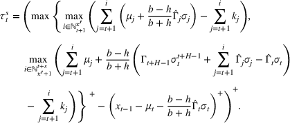
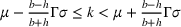
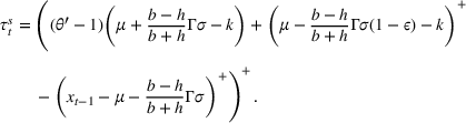
A key contribution of our work is to obtain an explicit expression of the shifting need. Including the worst‐case demand realizations derived using the symmetric uncertainty set (see Equation 5) into our expression of the shifting need results in:

Theorem 2 Shifting need for
$Ω^{sym}$

Let

μ_{i} - Γ_{i} σ_{i} > 0

for all

i \in N_{t}^{t + H - 1}

. Let

κ = \max {i : \sum_{j = t}^{i} {\hat{Γ}}_{j} σ_{j} \leq (Γ_{t + H - 1} σ_{t}^{t + H - 1} + \sum_{j = t}^{t + H - 1} {\hat{Γ}}_{j} σ_{j}) / 2}

, s be the shifting horizon and

κ^{'} = \min (κ, t + s)

, then

\begin{matrix} τ_{t}^{s} & = & (\max \{\max_{i \in N_{t + 1}^{κ^{'}}} (\sum_{j = t + 1}^{i} (μ_{j} + \frac{b - h}{b + h} {\hat{Γ}}_{j} σ_{j}) - \sum_{j = t + 1}^{i} k_{j}), \\ \max_{i \in N_{κ^{'} + 1}^{t + s}} (\sum_{j = t + 1}^{i} μ_{j} + \frac{b - h}{b + h} (Γ_{t + H - 1} σ_{t}^{t + H - 1} + \sum_{j = t + 1}^{i} {\hat{Γ}}_{j} σ_{j} - {\hat{Γ}}_{t} σ_{t}) \\ {- \sum_{j = t + 1}^{i} k_{j})\}^{+} - {(x_{t - 1} - μ_{t} - \frac{b - h}{b + h} {\hat{Γ}}_{t} σ_{t})}^{+})}^{+} . \end{matrix}

The expression of the shifting need simplifies in a stationary environment where both k is a constant and the demand in each period is independent and identically distributed with mean μ and standard deviation σ:

Corollary 3 Shifting need for
$Ω^{sym}$
(iid) and constant k

Let

μ - Γ σ > 0

. Let

θ = (H + \sqrt{H}) / 2, ε = θ - ⌊ θ ⌋

and let

θ^{'} = \min (s, ⌊ θ ⌋)

. Let

μ - \frac{b - h}{b + h} Γ σ \leq k < μ + \frac{b - h}{b + h} Γ σ

, then

\begin{matrix} τ_{t}^{s} & = & ((θ^{'} - 1) (μ + \frac{b - h}{b + h} Γ σ - k) + {(μ - \frac{b - h}{b + h} Γ σ (1 - ε) - k)}^{+} \\ {- {(x_{t - 1} - μ - \frac{b - h}{b + h} Γ σ)}^{+})}^{+} . \end{matrix}

The aforementioned expressions are in closed form but rely on the defined uncertainty set. Prior to applying our findings in practice, we first must provide parameterizations of the uncertainty set, which we do in Subsection 6.1 but first we provide some more analytical results related to the amount of shifting in various scenarios.

ANALYSIS OF THE ROBUST SOLUTION FOR THE CAPACITATED SYSTEM

Sensitivity of peak‐shaved quantity with respect to capacity changes

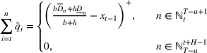
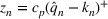
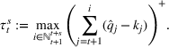
The Lookahead Peak‐Shaving policy shifts orders from future peak‐demand periods to the current period in order to avoid the sourcing cost premium. We denote the peak‐shaved quantity, that is, the amount of units shifted to the current period t compared to the uncapacitated system described in Subsection 4.1, as

Δ q_{t} : = q_{t}^{*} - {\hat{q}}_{t}

. This amount is dependent on how tight capacities are and how costly it is to source above the base capacity compared to the inventory mismatch costs. Figure 1b illustrates both the optimal order quantity

q_{t}^{*}

and the inventory‐dependent peak‐shaved quantity

Δ q_{t}

. In this section, we investigate how the amount of peak shaving varies under different capacity scenarios and for different capacity premiums. Below we outline our findings and focus on the related managerial implications, while a technical derivation of the results is provided in Appendix A in the Supporting Information.

The quantity of orders that can be peak shaved from future periods to the current period is determined by the current period's base capacity and the shifting need, denoted by

τ_{t}^{s}

, which depends on future capacities. If the current period's base capacity is tight, meaning that there is no capacity slack, no orders will be peak shaved to the current period. However, if there is capacity slack, orders will be peak shaved to the current period if there is a shifting need, that is, if future capacities are smaller than the optimal amount ordered in an uncapacitated system. In such cases, we can peak shave either the total shifting need, denoted by

τ_{t}^{s}

, if ample base capacity is available, or we can peak shave units until all spare capacity,

{(k_{t} - {\hat{q}}_{t})}^{+}

, is utilized. We have formalized these observations with respect to the current capacity in Proposition 1.

Proposition 1
For given capacities
$k_{t + 1}, …, k_{t + H - 1}$
the peak‐shaved quantity, that is, the amount shifted to period t from future periods, is given by
$Δ q_{t} = \min ({(k_{t} - {\hat{q}}_{t})}^{+}, τ_{t}^{s})$
.

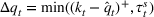
Figure 3a depicts the relationship between the current period's base capacity
$k_{t}$
(horizontal axis) and the peak‐shaved quantity (vertical axis), while holding future base capacities constant. Simply put, the more base capacity available in the current period, the more orders can be peak shaved from future periods to the current period. When the current period's base capacity is low, the uncapacitated order quantity already utilizes the entire base capacity, which means no further units can be peak shaved to the current period. However, if there is slack capacity, that is, if the base capacity exceeds the uncapacitated order quantity, all additional capacity can be utilized for peak shaving orders. Hence, increasing the current period's base capacity by one unit results in a corresponding increase in the peak‐shaved quantity, until the maximum amount that needs to be shifted, denoted by
$τ_{t}^{s}$
, is reached. Further increasing the base capacity beyond this point has no effect on the peak‐shaved quantity, indicating that adding more capacity is not beneficial when the current capacity is already high and sufficient future capacity is available. This suggests that most benefits of adding capacity occur when current capacity is low and when the shifting need is large, which is the case when future capacities are low. Such a scenario may occur for instance when capacity is tight for an upcoming weekend with large demand, such that having more capacity during the preceding week may allow the manufacturer to anticipate the busy weekend.

FIGURE 3
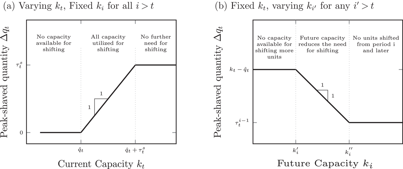
The peak‐shaved quantity for varying base capacities of the current period (panel a) or varying future capacities (panel b).

The peak‐shaved quantity is also dependent on the future capacity levels, as we show in Figure 3b. In general, higher future capacities decrease the amount that needs to be peak shaved as it reduces the shifting need. If there is peak shaving occurring for a given vector of base capacities, then reducing the capacity in a future period may (1) not change the amount peak‐shaved, if the current period's order already uses the base capacity, (2) reduce the amount peak‐shaved as future capacity becomes available and sourcing above base capacity in the current period is no longer needed (i.e., the shifting need becomes smaller than the slack available) or (3) not change the amount peak‐shaved, if the future capacity is already large enough to absorb all units shifted from that future period and later periods such that further increasing future capacity does not result in more peak shaving to the current period. Proposition 2 formalizes the relationship between the peak‐shaved quantity and base capacities. Proposition 2
Let the capacities in all periods of the planning horizon be given by
$k_{t}, k_{t + 1}, …, k_{H}$
. Let
$i^{'}$
be the period for which the shifting need obtains its maximum, that is,
$i^{'} = M (τ_{t}^{s})$
. Let i be a period that has direct impact on the shifting need, that is,
$i \in [t + 1, i^{'}]$
. Let
$k_{i}^{'}$
be the capacity in period i for which the shifting need
$τ_{t} (k_{i}^{'})$
is equal to the capacity slack available in period t, that is,
$τ_{t}^{i^{'}} (k_{i}^{'}) = k_{t} - {\hat{q}}_{t}$
and let
$k_{i}^{^{''}}$
be the capacity for which all units shifted in periods later than i can be absorbed, that is,
$k_{i}^{^{''}} = {\hat{q}}_{i} + {(\sum_{j = i + 1}^{i^{'}} ({\hat{q}}_{j} - k_{j}))}^{+}$
.

For any period
$i \in [t + 1, i^{'}]$
, the amount shifted to period t depends on the capacity
$k_{i}$
in period i as follows
$\begin{matrix} Δ q_{t} = \{\begin{matrix} 0, & k_{i} \leq {\hat{q}}_{i} \\ k_{t} - {\hat{q}}_{t}, & {\hat{q}}_{i} < k_{i} \leq k_{i}^{'} \\ τ_{t}^{i^{'}}, & k_{i}^{'} \leq k_{i} < k_{i}^{^{''}} \\ τ_{t}^{i - 1}, & k_{i}^{^{''}} \leq k_{i} \end{matrix} . \end{matrix}$

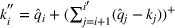
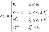
Figure 3b illustrates the scenario where future base capacities are increased while the current period's base capacity is held constant. We illustrate the case when we are currently peak shaving orders from period i to period t. Increasing the capacity in period i reduces the need to peak shave orders to period t. This might occur if carriers inform our manufacturer that slightly more transportation capacity will be available in the near future, temporarily increasing the base capacity for a future day. The increase of
$k_{i}$
results in a decreasing shifting need
$τ_{t}^{s}$
, as fewer units need to be peak shaved. Interestingly, at low future capacity levels, even though
$τ_{t}^{s}$
decreases, we observe no initial decrease on units being peak shaved. In that region, the base capacity of the current period is already fully utilized and an increased future capacity will not reduce the ordered amount (or equally the peak‐shaved amount). The order quantity will decrease linearly only when more future capacity (
$k_{i}^{'}$
in Figure 3b) becomes available. A unit increase in future capacity relates directly to a unit decrease in peak shaving. It is thus worth noting that not every small increase in future transportation capacity will necessarily reduce the amount of peak shaving for our manufacturer. At one point (
$k_{i}^{^{''}}$
in Figure 3b) there is sufficient capacity in period i such that no orders from i are peak shaved to period t. In addition, the base capacity in period i is large enough to also shift future demand peaks to period i instead of t. At this point the shifting need does not decrease anymore for an increase in capacity in i. It is only determined by period
$t + 1$
to
$t + i - 1$
alone.

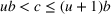
In addition to the role of the base capacities, the amount shifted is also dependent on the premium that is to be paid on flexible transportation supply. A larger premium of the transportation market encourages the manufacturer to peak shave more units to the current period, avoiding the future premium. The premium has an impact on the amount peak‐shaved by increasing the lookahead horizon. A higher premium leads to more periods being included in the lookahead horizon as it becomes beneficial to shift units forward by more periods. Proposition 3 formalizes this insight: Proposition 3
Let the lookahead horizon be
$s = ⌊ c_{p} / h ⌋$
. The lookahead horizon increases with increasing premium
$c_{p}$
. We denote by
$c_{p}^{'}$
the premium, for which the associated lookahead horizon is the first to exceed the capacity slack in period t, that is, the minimal
$c_{p}$
for which
$τ_{t}^{s} \geq k_{t} - {\hat{q}}_{t}$
, then
$Δ q_{t} = \{\begin{matrix} τ_{t}^{s} & for all c_{p} \leq c_{p}^{'} \\ {(k_{t} - {\hat{q}}_{t})}^{+} & for all c_{p} > c_{p}^{'} . \end{matrix}$

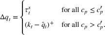
Figure 4 plots the peak‐shaved quantity
$Δ q_{t}$
as a function of the premium
$c_{p}$
. The cost premium affects the units shifted only by increasing the lookahead horizon (see Theorem 1). For example, if
$h < c_{p} \leq 2 h$
, it is only beneficial to move units from period
$t + 1$
to t. Shifting units from period
$t + 2$
to t incurs costs of 2h but only avoids costs of
$c_{p}$
that is not beneficial. If
$2 h < c_{p} \leq 3 h$
then shifting from period
$t + 2$
becomes beneficial. We thus observe a step‐wise function: as the penalty increases, it becomes attractive to peak shave from periods further in the future. This function is piece‐wise constant and increases (or stays constant) as the premium exceeds h,
$2 h, …, s h$
. Whether the amount shifted increases or not depends on the shifting needs
$τ_{t}^{s}$
that are related to a shifting horizon of s (s being equal to 1,2,3…).

FIGURE 4
Peak‐shaved quantity
$Δ q_{t}$
for different premium prices
$c_{p}$
.

At some point, however, any increase in the shifting need may not increase the units peak‐shaved, as the order quantity is capped by the base capacity of the current period
$k_{t}$
. This is indicated by the dashed line in Figure 4. The size of the step‐wise increases may vary as they are dependent on the future capacities and demand.

Analysis of the shifting need in nonstationary environments

Before performing an extensive numerical study, we demonstrate how the shifting need behaves in various settings with nonstationary demand. Figure 5 plots three settings of nonstationary demand (top panels) and the corresponding base‐stock levels and shifting need (bottom panels). For ease of exposition, all scenarios have a fixed capacity of 100 units per period (orange line, top panels). Given that the shifting need
$τ_{t}$
depends on
$x_{t - 1}$
, it is sample‐path dependent. To visualize it, we adopt an extreme case where we assume that
$x_{t - 1} = 0$
in each period and consider each point in time as the starting point of decision‐making, that is, we ignore past demand evolution. In Section 6, we do carry over inventory when evaluating the cost performance of the Lookahead Peak‐Shaving policy.

FIGURE 5
We show for three settings with nonstationary demand (top panels) how the base‐stock levels and shifting need (bottom panels) anticipates changes in demand. The shifting need decreases when future demand is low, and vice versa. This anticipative behavior explains the strong numerical performance of our numerical experiment in Section 6. Note: We use the following parameters:
$h = 1$
,
$b = 9$
,
$c = 0$
,
$c_{p} = 4$
,
$\hat{Γ} = 2$
,
$Γ = 2$
.

The top panel of Figure 5a corresponds to a scenario with alternating sequences of high and low demand. The standard deviation is constant. The bottom panel of Figure 5a shows the corresponding low base‐stock level (circles), high base‐stock level (triangle) and the shifting need (length of the blue line). The shifting need thus corresponds to the volume that would be shifted forward, if sufficient base capacity is available in the current period and the inventory is below the low base‐stock level. The lower base‐stock levels (circles) are constant over the periods where the demand is constant (periods 1–10, 11–20, …). It equals the robustly optimal base‐stock level of the uncapacitated system. The upper base‐stock level (triangles) shows the key dynamics of the robust Lookahead Peak‐Shaving policy. In high demand periods, the upper base‐stock level is high as more units are peak shaved, if base capacity is available. If the expected demand drops within the shifting horizon, less orders are peak shaved. The shifting horizon in this example is four periods, thus the high base‐stock level decreases in periods 7–10 and 27–30, four periods before the expected demand drops. At the same time, when the expected demand raises within the shifting horizon, more orders are peak shaved. We note that the actual peak‐shaved quantity is dependent on the demand realizations. The shifting need only indicates the amount that shall be shifted to earlier periods, if base capacity is available. Thus, the shifting need anticipates drops (raises) in the expected demand, and decreases (increases) as a result to decrease (increase) the amount shifted forward in low (high) demand period.

The same pattern arises, when we keep the expected demand constant and vary the standard deviation over time (Figure 5b). In this case, the pattern for periods with high demand uncertainty resembles the pattern for periods with high expected demand in Figure 5a. Peak shaving increases for periods with high uncertainty and reduces for periods with low uncertainty (Figure 5b, bottom panel). In this way, additional inventory is kept when higher uncertainties are expected over the shifting horizon.

Figure 5c illustrates a cyclic mean but constant coefficient of variation. The lower base‐stock level follows the same pattern as the expected demand curve. We observe how the upper base‐stock level and the shifting need exhibit a similar pattern as the demand, but one shifted forward. The demand curve exhibits peaks (valleys) in periods 6, 26, and 46 (16 and 36) and the upper base‐stock level exhibits peaks (valleys) in periods 4, 24, and 44 (14 and 34). Thus, the upper base‐stock level exhibits the peaks (valleys) when the cumulative expected demand over the shifting horizon reaches its peak (valley). In those periods, the most (the least) is supposed to be peak shaved.

NUMERICAL EXPERIMENT

We first perform an extensive numerical study where we let demand be nonstationary and correlated, and capacities fluctuate. Subsequently, we show the performance using a real data set of a manufacturer. In all settings, the evaluation criterion is the conventional expected cost rather than the worst‐case cost realizations.

Tuning the uncertainty set for practical implementation

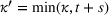
The remaining challenge in utilizing our robust Lookahead Peak‐Shaving policy is fine‐tuning the uncertainty parameter sets
$Γ_{t}$
and
${\hat{Γ}}_{t}$
. To avoid the computational burden to optimize these values, we propose to keep the period‐dependent values of both sets equal in each period. Formally, we introduce two constants, Γ and
$\hat{Γ}$
, and set
$Γ_{i} = Γ$
and
${\hat{Γ}}_{i} = \hat{Γ}$
for all i in
$N_{t}^{t + H - 1}$
, respectively. This is appealing as it reduces the search space from two times the length of the planning horizon (2H) to only two dimensions. We thus search over Γ and
$\hat{Γ}$
from which the respective base‐stock levels directly follow as per Theorem (1) and Corollaries (3) and (5). We use the symmetric (asymmetric) uncertainty set when
$μ_{i} - Γ σ_{i} \geq 0$
(
$μ_{i} - Γ σ_{i} < 0$
). This way we capture that demand is strictly nonnegative.

The Lookahead Peak‐Shaving policy is optimal when demand is stationary and not correlated, and when capacity does not fluctuate: Γ and
$\hat{Γ}$
can be set such that the resulting base‐stock levels coincide with the optimal ones (which are stationary as long as the planning horizon is sufficiently long to discard end‐of‐horizon effects). The strength of our results, however, stems from applying our closed‐form expressions in more complex environments where demand is correlated and nonstationary, and where capacities fluctuate.

Two benchmark heuristics

To demonstrate the numerical performance of the Lookahead Peak‐Shaving policy, we construct two benchmark heuristics. Both adopt the optimal policy structure but set the base‐stock levels differently. First, we propose the z‐score policy that uses the first two moments as follows:
$S_{t}^{1} = μ_{t} + z_{1} σ_{t}$
and
$S_{t}^{2} = μ_{t} + z_{2} σ_{t}$
. Both z ₁ and z ₂ are constants that we optimize using full enumeration: Definition 3 The z‐score policy

Set

S_{t}^{1} = μ_{t} + z_{1} σ_{t}

and

S_{t}^{2} = μ_{t} + z_{2} σ_{t}

for all periods where z ₁ and z ₂ are tunable parameters.

In practice, this corresponds to a policy that sets the base‐stock levels using the forecast and its error. The z‐score policy, however, does not take into account future period's demand that may limit its performance in several settings. Hence, we also compare our policy against an alternative benchmark that is forward‐looking: the days‐of‐sales policy where we compute the base‐stock levels using the expected days‐of‐sales, which we label the days‐of‐sales policy:

Definition 4 The days‐of‐sales policy

Set

S_{t}^{1} = \sum_{i = t}^{t + ⌊ m_{1} ⌋ - 1} μ_{i} + (m_{1} - ⌊ m_{1} ⌋) μ_{t + ⌊ m_{1} ⌋}

and

S_{t}^{2} = \sum_{i = t}^{t + ⌊ m_{2} ⌋ - 1} μ_{i} + (m_{2} - ⌊ m_{2} ⌋) μ_{t + ⌊ m_{2} ⌋}

for all periods where m ₁ and m ₂ are tunable parameters.

In contrast to the z‐score benchmark policy, the days‐of‐sales policy incorporates, and adapts to, future fluctuations in demand. In contrast to the z‐score benchmark policy, the days‐of‐sales policy incorporates, and adapts to, future fluctuations in demand. However, note that the days‐of‐sales policy only depends on the expected demand in a period (first moment) and not its variability (second moment). Thus, either policy can dominate depending on whether the first or second moment fluctuations dominate. In our numerical experiment, we will show the value of our Lookahead Peak‐Shaving policy compared to both benchmark policies.

Performance on synthetic data set

We set the unit holding cost

h = 1

and scale all other costs in relation to the unit holding cost without loss of generalization. We set the unit backlog cost

b = 9

to reflect a service level of 90%. The regular sourcing cost c is set to zero as the unit cost c is always incurred per unit ordered. Finally, the premium cost is set to

c_{p} = 4

in line with Assumption 1.

Each period, the Lookahead Peak‐Shaving policy is optimized over a rolling horizon of

H = 10

periods, of which only the first order is implemented. We minimize the long‐run expected cost of the Lookahead Peak‐Shaving policy, the z‐score policy, and the days‐of‐sales policy by simulating 10 × 10,000 periods. We report the improvement of our Lookahead Peak‐Shaving policy over both benchmark policies over these 10 long sample paths and include confidence bounds at the 95% confidence level.

Impact of fluctuating the mean demand and capacities

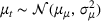
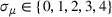
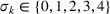
We first focus on the impact of fluctuating demand and capacities that we model as follows: The demand in each period t follows a Gamma distribution with a nonstationary mean per period

μ_{t}

and a constant standard deviation

σ = 2

. This corresponds to a different forecast in each period but identical forecast errors. We simulate nonstationarity by sampling the mean from a normal distribution:

μ_{t} \sim N (μ_{μ}, σ_{μ}^{2})

. We fix the overall mean at

μ_{μ} = 10

and vary the standard deviation of the periodic means

σ_{μ} \in {0, 1, 2, 3, 4}

to simulate different degrees of nonstationarity. The capacity in each period t fluctuates around the mean demand and is sampled from a normal distribution:

k_{t} \sim N (μ_{t}, σ_{k}^{2})

. We thus let the capacity fluctuate around the mean demand and vary the standard deviation of the capacity

σ_{k} \in {0, 1, 2, 3, 4}

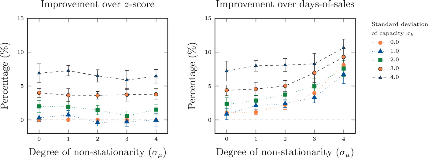
In Figure 6, we present the performance improvement of the Lookahead Peak‐Shaving policy over our two benchmark policies: the z‐score policy (left panel) and the days‐of‐sales policy (right panel). We observe that the Lookahead Peak‐Shaving policy outperforms both policies. While increasing the degree of nonstationarity does not impact the performance gap with the z‐score policy (from left to right on the left panel) we do see the performance gap widening compared to the days‐of‐sales policy (from left to right on the right panel). The Lookahead Peak‐Shaving policy anticipates changes in capacities better than both benchmark policies. The performance gap clearly increases when capacities fluctuate more (lines corresponding to larger fluctuations in capacity are higher in both panels).

FIGURE 6

We observe that the Lookahead Peak‐Shaving policy outperforms the z‐score policy (left panel). The performance gap stays similar when demand fluctuates more but the gap clearly increases for larger fluctuations in the capacity as it better anticipates fluctuating capacity. The Lookahead Peak‐Shaving policy performs better than the days‐of‐sales policy, with an increasing performance gap both when demand and capacities fluctuate more (right panel).

We allot the excellent performance of the robust policy to its ability to better anticipate differences between future demand and contracted capacity. Consequently, it can more efficiently decide when to advance orders in order to avoid future overtime premiums. The opportunities for leveraging this forward‐looking feature increase when the degree of nonstationarity increases and when capacities fluctuate. We conclude that the robust Lookahead Peak‐Shaving policy seems to perform well in comparison to the benchmark policies, also when evaluated against the expected cost criterion.

Impact of demand correlation and variability

We also investigate the impact of demand correlation and variability. We model demand to be correlated according to an AR(1) process with correlation coefficient

ρ \in {- 0.5, 0, 0.5}

. We let the standard deviation of the demand vary

σ \in {0, 1, 2, 3, 4}

. Figure 7 demonstrates the improvement of the Lookahead Peak‐Shaving policy over the z‐score policy (left panel) and the days‐of‐sales policy (right panel).

FIGURE 7

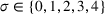
The Lookahead Peak‐Shaving policy performs best when demand is negatively correlated and when demand variance is small. In these cases, it can better anticipate future capacities and demand.

We first note that the Lookahead Peak‐Shaving policy is optimal when demand is deterministic as in this case the worst‐case bounds are equal and solving the linear program, as in Equation (4), yields the optimal order quantities. We observe strong cost improvement of +40% compared to the z‐score and +25% compared to the days‐of‐sales policy when the standard deviation is (close to) zero. Increasing the standard deviation reduces the improvement, as computing the shifting need becomes gradually less accurate due to an increased forecast error. Yet, even for large values of the standard deviation, the Lookahead Peak‐Shaving policy yields good results, especially when demand is negatively correlated. Negative correlation reduces the demand variance in the next periods such that the Lookahead Peak‐Shaving policy has access to a tighter estimation of future demand. In conclusion, most benefits arise when demand and capacities fluctuate and when the demand variance is small, allowing smarter shifting.

Performance on a real data set

We also investigate the performance of our policy on real data of a manufacturer in the consumer‐goods industry. Its shipments between plant and warehouse are outsourced to dedicated transportation carriers. Daily available transportation capacities may be exceeded on a given day by resorting to the freight auction market that comes at a premium.

Our data set contains demand and forecast information of 869 stock keeping units (SKUs) for a time span of approximately 3 months, covering the fourth quarter of 2019 (hence no Covid‐19 impact). For each SKU we possess the demand realizations and for each day and SKU, we have the forward‐looking demand forecasts for each of the next 40 days. The forecast includes both the output of advanced statistical tools and judgmental adjustments made by demand planners that interact closely with marketing and sales. Although the forecast accuracy of monthly demand is rather good with forecast errors (mean average percentage errors) typically below 10%, the forecasts of daily demands show larger errors as large key account orders may arrive several days earlier or later compared to the original forecast. This fits well with the uncertainty set that can allow for large periodic deviations, but can force the sum over several periods to have a small deviation. We split our data set that contains 3 months of data into a training set to optimize all policy parameters (the first 1.5 months), and a test set to evaluate the policies (the subsequent 1.5 months).

We apply the Lookahead Peak‐Shaving policy and compare it to the same two benchmark policies as the previous section. We describe how we retrieved the empirical moments from the data in detail in Appendix C in the Supporting Information. Each product has its own pre‐dedicated, and fixed, capacity that we set equal to the mean of each product across all periods within the training set. This mimics how the manufacturer typically negotiates capacity around (or slightly above) the average daily shipment size while shipments exceeding this pre‐dedicated capacity are made on the freight auction market. We use the same product‐specific capacities for the evaluation set.

For each SKU, we use the training set to obtain the policy parameters, that is, Γ and

\hat{Γ}

for the robust policy, z ₁ and z ₂ for the z‐score policy, and m ₁ and m ₂ for the days‐of‐sales policy. We optimize the policy parameters per product individually.

We report the cost performance of the Lookahead Peak‐Shaving policy and both benchmark policies in Figure 8 using a Pareto plot, where we rank the products from largest volume to smallest. The numerical parameters we used are as follows. We keep

h = 1

and

c = 0

and set the service level to 90%, corresponding to

b = 9

. Finally, we set the constant freight auction premium range to

c_{p} = 2

. We note that choosing higher premiums only increases the performance of the Lookahead Peak‐Shaving policy. We plot the cumulative cost of all policies, and normalize around the total cost of the Lookahead Peak‐Shaving policy. We see that the z‐score policy increases costs by 6.7%. The days‐of‐sales policy performs worst, increasing the cost by more than 40%. We attribute this to the observations we made on the synthetic data set: as our data set's demand fluctuates significantly and some SKUs' demand is very intermittent, the days‐of‐sales policy lacks flexibility to cope with the demand variability.

FIGURE 8

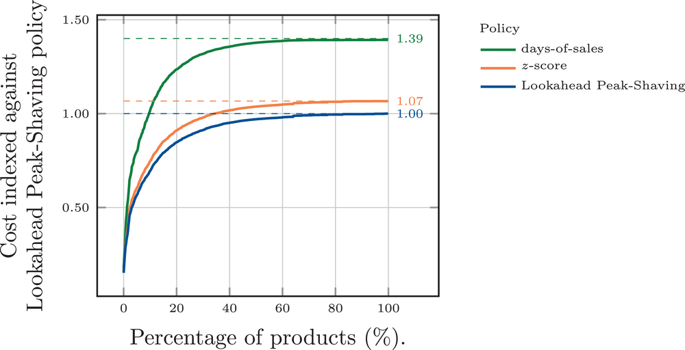
Pareto plot. Products ranked according to size. Here we can see for the percentage of largest products, how much they contribute to the total cost. All costs indexed around the Lookahead Peak‐Shaving policy.

We conclude that for the full portfolio the Lookahead Peak‐Shaving policy can clearly outperform the current policy adopted by the manufacturer.

CONCLUSION

We studied the robustly optimal replenishment policy in a single sourcing backlogging system with volume flexibility. Sourcing costs are piece‐wise linear and convex with an additional premium incurred once a pre‐dedicated threshold is exceeded. This setting corresponds to various contexts, for example, factories typically have a dedicated workforce but can temporarily exceed this capacity by exploiting overtime labor, companies can choose from several suppliers with individual capacity constraints and different unit costs or firms can book dedicated transportation capacity with an option to use the transportation spot market. We adopt a robust formulation and prove that the robustly optimal policy has the same structure as the stochastically optimal policy. The robust base‐stock levels are characterized by the robustly optimal base‐stock level of the uncapacitated system and an explicit expression of the shifting need that determines when orders should be advanced to earlier periods to avoid the overtime premium. We term the resulting policy the Lookahead Peak‐Shaving policy as it peak shaves orders from future peak‐demand periods to the current periods. We compare our policy against two benchmark heuristics and find that our policy performs well, also when evaluated against the expected costs; especially in settings characterized by high fluctuations of the periodic capacity, of the expected demand, or of both. We affirmed these findings by applying our model on data of a manufacturer. The robust policy saves 6.7% compared to the policy currently used by the manufacturer. In conclusion, our closed‐form expressions facilitate adoption in practice, they generate intuitive insights for managers into the dynamics of the problem and their application on real data results in substantial savings.

Footnotes

ORCID

Joren Gijsbrechts

Christina Imdahl

Robert N. Boute

Jan A. Van Mieghem

References

Ardestani‐Jaafari

Delage

(2016). Robust optimization of sums of piecewise linear functions with application to inventory problems. Operations Research, 64(2), 474–494.

Bandi

Bertsimas

(2012). Tractable stochastic analysis in high dimensions via robust optimization. Mathematical Programming, 134(1), 23–70.

Ben‐Tal

El Ghaoui

Nemirovski

(2009). Robust optimization, (vol. 28). Princeton University Press.

Berger

(2021). Where did all the shipping containers go? https://www.wsj.com/articles/where‐did‐all‐the‐shipping‐containers‐go‐11628104583

Bertsimas

Sim

(2004). The price of robustness. Operations Research, 52(1), 35–53.

Bertsimas

Thiele

(2006). A robust optimization approach to inventory theory. Operations Research, 54(1), 150–168.

Bhattacharjee

Bustamante

Curley

Perez

(2021). Navigating the labor mismatch in us logistics and supply chains . https://www.mckinsey.com/business‐functions/operations/our‐insights/navigating‐the‐labor‐mismatch‐in‐us‐logistics‐and‐supply‐chains

Gijsbrechts

Boute

R. N.

Disney

S. M.

Van Mieghem

J. A.

(2022). Volume flexibility at responsive suppliers in reshoring decisions: Analysis of a dual sourcing inventory model. Production and Operations Management, 00, 1–20. https://doi.org/10.1111/poms.13719

Gorissen

B. L.

Den Hertog

(2013). Robust counterparts of inequalities containing sums of maxima of linear functions. European Journal of Operational Research, 227(1), 30–43.

10.

Henig

Gerchak

Ernst

Pyke

D. F.

(1997). An inventory model embedded in designing a supply contract. Management Science, 43(2), 389–403.

11.

Karlin

(1958). Chapter 8: One‐stage inventory models with uncertainty. Studies in the mathematical theory of inventory and production (pp. 340). Stanford University Press.

12.

Karlin

Scarf

(1958a). Chapter 10: Inventory models of the arrow‐Harris–Marschak type with time lag. Studies in the mathematical theory of inventory and production (pp. 340). Stanford University Press.

13.

Karlin

Scarf

(1958b). Studies in applied probability and management science. Stanford University Press.

14.

Krauss

(2022). Why are oil prices so high and will they stay that way? https://www.nytimes.com/2022/02/02/business/economy/oil‐price.html

15.

Song

(2014). Inventory control with a fixed cost and a piecewise linear convex cost. Production and Operations Management, 23(11), 1966–1984.

16.

Mamani

Nassiri

Wagner

M. R.

(2017). Closed‐form solutions for robust inventory management. Management Science, 63(5), 1625–1643.

17.

Martínez‐de Albéniz

Simchi‐Levi

(2005). A portfolio approach to procurement contracts. Production and Operations Management, 14(1), 90–114.

18.

Porteus

(1990). Stochastic inventory theory. Handbooks in Operations Research and Management Science, 2, 605–652.

19.

Soyster

(1973). Convex programming with set‐inclusive constraints and applications to inexact linear programming. Operations Research, 21(5), 1154–1157.

20.

Sun

Van Mieghem

J. A.

(2019). Robust dual sourcing inventory management: Optimality of capped dual index policies. Manufacturing & Service Operations Management, 21(4), 912–931.

21.

Tyagi

Lademan

Verma

Holt

(2021). Early 2022‐23 contract discussions see container rates surge, terms evolve. https://www.spglobal.com/platts/en/market‐insights/latest‐news/shipping/121021‐early‐2022‐23‐contract‐discussions‐see‐container‐rates‐surge‐terms‐evolve

22.

Wagner

(2018). Robust inventory management: An optimal control approach. Operations Research, 66(2), 426–447.

23.

Xin

Goldberg

D. A.

(2018). Asymptotic optimality of tailored base‐surge policies in dual‐sourcing inventory systems. Management Science, 64(1), 437–452.

Supplementary Material

Please find the following supplemental material available below.

For Open Access articles published under a Creative Commons License, all supplemental material carries the same license as the article it is associated with.

For non-Open Access articles published, all supplemental material carries a non-exclusive license, and permission requests for re-use of supplemental material or any part of supplemental material shall be sent directly to the copyright owner as specified in the copyright notice associated with the article.

0.00 MB

0.29 MB

Optimal robust inventory management with volume flexibility: Matching capacity and demand with the lookahead peak‐shaving policy

Abstract

Keywords

INTRODUCTION

RELATED LITERATURE

MODEL OF CAPACITATED SOURCING WITH VOLUME FLEXIBILITY

Stochastic model

Robust model

SOLUTION OF THE ROBUST MODEL

Solution for the uncapacitated system

Solution for the capacitated system

Theorem 2 Shifting need for Ω sym $\Omega ^{\text{sym}}$

Corollary 3 Shifting need for Ω sym $\Omega ^{\text{sym}}$ (iid) and constant k

ANALYSIS OF THE ROBUST SOLUTION FOR THE CAPACITATED SYSTEM

Sensitivity of peak‐shaved quantity with respect to capacity changes

Analysis of the shifting need in nonstationary environments

NUMERICAL EXPERIMENT

Tuning the uncertainty set for practical implementation

Two benchmark heuristics

Definition 4 The days‐of‐sales policy

Performance on synthetic data set

Impact of fluctuating the mean demand and capacities

Impact of demand correlation and variability

Performance on a real data set

CONCLUSION

Footnotes

ORCID

References

Supplementary Material

Theorem 2 Shifting need for
$Ω^{sym}$

Corollary 3 Shifting need for
$Ω^{sym}$
(iid) and constant k