Sage Journals: Discover world-class research

Abstract

This study examines human ordering behavior in service‐level inventory contracts, a class of contracts important in practice. Studies of wholesale price contracts find that people tend to place orders that are suboptimal and biased toward mean demand. Unlike wholesale price contracts, service‐level contracts can be parameterized such that they have steep expected profit functions, making the expected profit‐maximizing order more salient, in the sense that deviations from optimal ordering are more costly. Utilizing an analytical model and results from existing literature, we hypothesize that people will order closer to optimality under service‐level contracts with steeper expected profit functions. In a laboratory experiment, we find that subjects achieve up to 97.2% supply chain efficiency under a steep service‐level contract, compared with 92.2% under a flat service‐level contract, and steep service contract ordering also exhibits lower variability. Our results suggest that managers can benefit by designing service‐level contracts with higher penalty costs and lower fill rates.

Keywords

behavioral operations experimental economics service‐level contracts

INTRODUCTION

This paper investigates inventory ordering behavior under service‐level contracts. Service‐level contracts are common in practice (Behrenbeck et al., 2003; Chen & Thomas, 2018; Liang & Atkins, 2013; Sieke et al., 2013). They incentivize order fulfillment by stipulating a level of demand fulfillment (the fill target) and a penalty if it falls below the target level, together with a wholesale price. In theory, there are often multiple ways to parameterize a service‐level contract to achieve a desired optimal ordering quantity (Sieke et al., 2013, and references therein). Our findings will suggest that certain of these parameterizations are better than others at inducing optimal ordering in human decision‐makers.

Studies of decision making under other types of inventory contracts find broad‐based suboptimal behavior. Wholesale price contracts, which simply specify a wholesale price, induce order quantities that exhibit a “pull‐to‐center” effect in which observed average order quantities are regularly between the expected profit‐maximizing quantities and mean demand. The effect is highly robust and extends to buyback and revenue‐sharing contracts; Becker‐Peth and Thonemann (2018) and Chen and Wu (2018) survey this large literature. Few of these studies are concerned with service‐level contracts. Katok et al. (2008) and Davis (2015) are exceptions, although their focus differs from ours. Katok et al. (2008) study the performance of service‐level agreements and focus on the influence of the review period over which the fill rate is calculated in a pull setting, while Davis (2015)—in a similar pull setting—concentrates on the structural biases of the retailer when proposing the parameters of a service‐level agreement to a supplier who makes the order‐up‐to‐level decision.

Service‐level contracts are more complex than wholesale price contracts in terms of the number of parameters. Yet, a reason to suspect that service‐level contracts can induce more optimal ordering than wholesale price contracts is that the financial parameters of service‐level contracts can be chosen to make the optimal order quantity more “salient” in the sense that a small deviation from the optimum order leads to a higher expected loss in profit. Higher salience increases the cost of pursuing nonmonetary objectives (Harrison, 1989) and can increase the speed of reinforcement adaptive learning (Bostian et al., 2008; Erev & Roth, 1998). Studies of performance in other kinds of decision tasks find that heightened salience can lead to more optimal decisions (e.g., Davis et al., 2003; Harrison, 1989; Potters & Suetens, 2020), although others do not (e.g., Romeo & Sopher, 1999).

Wholesale price contracts analyzed in the behavioral literature tend to have expected profit functions with low salience about the optimum order. For example, Schweitzer and Cachon (2000) study contracts in which order quantities that deviate by 10% from the optimal quantities achieve expected profits that deviate only about 1% from the maximum expected profit. Wholesale price contracts cannot be manipulated to increase salience, as the desired optimal order quantity is held fixed (the available parameters are insufficient as explained below). Service‐level price contracts can.

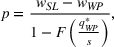
We conducted an experiment to see whether service‐level contracts with greater salience lead to ordering decisions closer to those that are theoretically optimal. We also compared the performance of these contracts to that of the corresponding wholesale price contract. We use an analytical model to determine the contract parameters that incentivize optimal order quantities for expected profit‐maximizing retailers and conduct laboratory experiments with these contracts. We find that service‐level contracts can achieve high efficiency if they are parameterized for a steep expected profit function. This can be achieved by choosing a unit penalty cost of providing fewer units than agreed on that is high relative to the margin of the product. Average order quantities are then closer to the expected profit‐maximizing quantity and have lower variability than those under a wholesale price contract. In our experiment, the efficiency under the steepest service‐level contract is up to 97.2%, compared with an efficiency of 92.2% under the flat service‐level contract (and 88.2 % under the wholesale price contract).

Ho et al. (2010) presented theory and data to show that the salience of psychological costs associated with over‐ and under‐ordering can explain the pull‐to‐center effect observed in newsvendor experiments. Our data show that increasing the salience of the economic costs of service‐level contracts can induce a debiasing effect.

In practice, there is little agreement on the right approach to choosing the penalty associated with missing the fill target. Alicke (personal communication, July 29, 2019) observes that companies do not have a good understanding of how the parameters of the contracts should be specified. While the service levels used in these contracts often seem to be set based on industry benchmarks (e.g., 70% for perishable products in retailing, 99% for key components in manufacturing), companies do not seem to follow a common or consistent approach for setting financial penalties. Some use no financial penalties, while others use substantial penalties for missing agreed‐on service levels (e.g., Mostberger, 2006) or require, for instance, financial compensation for the downtime of a manufacturing process or to cover the cost of emergency shipments. Behrenbeck et al. (2005) analyze the supply chain performance of 33 large companies in the European consumer goods industry and clustered the companies into two groups: a group that achieves high supply chain performance (champions) and a group that does not (followers). They reported that 83% of the champions measured their partners’ service levels, and 40% of the champions enforced financial penalties if a prespecified target was not met. Among the followers, only 59% measured service levels and only 5% enforced financial penalties.

From what we can infer from publicly available contracts and conversations with practitioners is that penalties range between 1% of the retail price (e.g., for grocery settings where the service level is on the supplier's side and based mostly on a lost margin) and 500% of an entire period's contractual payment amount (e.g., in outsourcing settings where the provider maintains relevant network structures).¹

Our analyses suggest that managers would do well to set enforced penalties for missing the service‐level target and to set them relatively high. Our data provide evidence that salience explains the difference we observe in performance among service‐level contracts and that service‐level contracts that exhibit high salience outperform comparable wholesale price contracts. A precise statement of the mechanism behind the transition from wholesale to service‐level performance—whether salience alone is the determinate factor or other factors are at play—requires study beyond the scope of this paper. The findings here establish a foundation for pursuing such an agenda and suggest candidate factors to be examined.

THEORETICAL ANALYSIS OF THE SERVICE‐LEVEL CONTRACT

Our primary interest is to understand the ordering behavior of a decision‐maker under a service‐level contract. The decision‐maker can be, for instance, a supplier who has made an agreement with a retailer to fulfill a certain fraction of the retailer's orders, or a retailer who made an agreement with a supplier to achieve a certain service level of the supplier's products in her store. The latter setting is for instance relevant in the consumer goods industry, where consumer goods producers are interested in having high on‐shelf availability of their products at the retailers. We consider this setting in our model and note that our results hold generally for decision making under service‐level contracts.

Consider a retailer who chooses order quantity q and places an order with the supplier. When determining the order quantity, the retailer knows the distribution F(D) of demand D but not the demand realization d. For our analyses, we assume that the demand density f(D) is log‐concave and has strictly positive support on its entire domain. Most distribution functions commonly used in inventory management have this property (Rosling, 2002), and it simplifies our theoretical analyses. The supplier produces order quantity q and delivers it to the retailer at the unit wholesale price w. The retailer sells the minimum of the order quantity q and demand d to customers at unit revenue r. Excess inventory has no salvage value, and excess demand is lost. We refer to the order quantity that maximizes the retailer's expected profit as the optimal order quantity and next show how it can be determined for wholesale price and service‐level contracts.

A wholesale price contract has a single parameter, the unit wholesale price w. For order quantity q and demand realization d, the retailer's profit is

π_{W P} (w, q, d) = r \min (q, d) - w q .

The optimal order quantity is (Arrow et al., 1951):

q_{WP}^{*} (w) = F^{- 1} (\frac{r - w}{r}),

and we denote the optimal expected profit as

Π_{W P}^{*} (w) = E [π_{W P} (w, q_{W P}^{*} (w), d)]

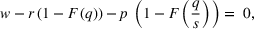
A service‐level contract specifies the fraction of demand that the retailer is obligated to fill and the financial consequences of failing to do so. The fraction of demand that must be filled is referred to as the service level s. For a demand realization of d units, the retailer must fill at least sd units. If the retailer ordered fewer than sd units, a unit penalty cost of p is charged for each unit difference between sd and q. If the retailer ordered at least sd units, no penalty is charged. For order quantity q and demand realization d, the retailer's profit is:

π_{S L} (s, p, w, q, d) = r \min (q, d) - w q - p {(s d - q)}^{+} .

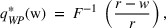
The retailer's optimal order quantity

q_{S L}^{*} (s, p, w)

can be determined by solving (Sieke et al., 2013)

w - r (1 - F (q)) - p (1 - F (\frac{q}{s})) = 0,

and we denote the optimal expected profit as

Π_{S L}^{*} (s, p, w) = E [π_{S L} (s, p, w, q_{S L}^{*} (s, p, w), d)]

It is not possible to change the slope of the expected profit function for regular wholesale price contracts without also changing the targeted optimal solution. To see this, note that the critical fractile (r‐w)/r in Equation (2) shifts when either parameter r or w is changed. Only if r and w are changed by the same multiplicative factor will the critical fractile not be changed. But multiplying the retail price r is often infeasible in practice. Increasing the salience of a given optimal order requires a different kind of contract.

The service‐level contract has three parameters. Observe from Equation (4) that a given optimal order quantity can be achieved by different combinations of the contract parameters. For instance, consider a supplier with a unit production cost of c = 3, a unit revenue of r = 12, and uniformly distributed customer demand between 1 and 100. The expected supply chain profit‐maximizing order quantity is 75 units. For a service‐level contract with unit wholesale price w = 6 and unit revenue of r = 12, Figure 1 depicts the combinations of service level s and unit penalty cost p for a retailer's optimal order quantity of 75 units; for example, service level s = 75% and unit penalty cost p = 145, service level s = 100% and unit penalty cost p = 12, or any combination of service level and unit penalty cost on the curve.

FIGURE 1

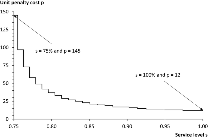
Combinations of service levels and unit penalty costs incentivizing an optimal order quantity of 75

Although the order quantity that maximizes expected profit is the same for all combinations of s and p on the curve, the expected profit functions are different. For the extreme cases, that is, for s = 75% and p = 145 and for s = 100% and p = 12, the retailer's expected profit functions are depicted in Figure 2a. The expected profit function of the wholesale price contract, which we will use as a benchmark, is also shown. The graphs show that the contracts have the same optimal order quantities but different optimal expected profits. For our analyses, we scale the contracts such that they have the same optimal expected profits. We add

π_{W P}^{*} (w)

−

π_{S L}^{*} (s, p, w)

to the profit function

π_{S L} (s, p, w, q, d)

of Equation (3). The results are shown in Figure 2b.

FIGURE 2

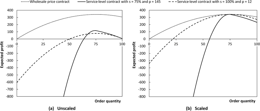
Retailer's expected profit functions for different contracts with optimal order quantity of 75

The graphs in Figure 2b indicate that the service‐level contract with a low service level and a high unit penalty cost (s = 75%, p = 145) has a steeper expected profit function than that with a high service level and a low unit penalty cost (s = 100%, p = 12) and show that both service‐level contracts have steeper expected profit functions than the wholesale price contract. The hypotheses that we derive below are based on such observations. We consider wholesale price contracts with wholesale prices

0 < w_{W P} < r

and optimal and service‐level contracts with service levels

0 < s < 1

and wholesale prices

w_{S L} > w_{W P}

. When comparing the performance of service‐level contracts and wholesale price contracts, we choose a unit penalty cost of

p = \frac{w_{S L} - w_{W P}}{1 - F (\frac{q_{W P}^{*}}{s})},

such that the service‐level contract has the same optimal order quantity as the wholesale price contract. We refer to contracts with the same optimal order quantities as corresponding contracts.

A property of the expected profit function that is relevant to our hypothesis development is its steepness. The steeper the expected profit function is, that is, the higher the absolute value of its first derivative is, the more costly the deviations from the optimal order quantities are. The following proposition addresses the steepness of the contracts: Proposition 1

Service‐level contracts have steeper expected profit functions than the corresponding wholesale price contracts.

Expected profit is also affected by order variability. The effect of order variability on expected profit depends on the concavity of the expected profit function. For concave profit functions, the marginal profit loss that is incurred by deviating from the optimal order quantity is increasing in the distance between the order quantity and the optimal order quantity. The more concave the expected profit function is, that is, the higher the absolute value of its second derivative is, the greater the effect of order variability on expected profits. The following proposition compares the concavity of wholesale price contracts and service‐level contracts: Proposition 2

Service‐level contracts have more concave expected profit functions than the corresponding wholesale price contracts.

We refer the reader to Appendix A for proofs of Proposition 1 and Proposition 2.

DEVELOPMENT OF HYPOTHESES

In newsvendor‐related experiments, actual order quantities deviate from the optimal order quantities and exhibit substantial variability, which results in expected profits that are substantially below the maximum expected profits (Becker‐Peth & Thonemann, 2018). For example, the expected profits under a wholesale price contract in the baseline treatments of Bolton et al. (2012) are 13.3% below optimality. In their experiment, approximately one‐half of the performance gap can be attributed to deviations of actual average orders from optimal order quantities and one‐half to order variability. Other studies have reported similar results (e.g., Rudi & Drake, 2014), which indicates that two issues must be addressed to achieve efficient ordering behavior: Average orders must be close to optimal quantities and must exhibit low variability.

Salience of optimal order quantity

Bostian et al. (2008) hypothesized that suboptimal ordering behavior can be attributed to the flatness of the expected profit function: “The flatness of the expected profit function in the neighborhood of [

q^{*}

] implies a low average payoff penalty for choosing an order quantity that is merely close to the optimum. As a result, subjects may not have an economic incentive to be very circumspect in their decisions, and so lazy decision making could possibly explain the pull‐to‐center effect” (p. 593). For references to salience studies on other games, see the Introduction section.

Bolton and Katok (2008) offered similar arguments. They argued that the wholesale price contract, which has an expected profit function that is flat around the maximum, provides low salience of the optimal solution. Then, it is difficult for decision‐makers to identify optimal order quantities based on outcomes. They tend to rely on suboptimal heuristics and learning; if present at all, learning is slow. Bolton and Katok (2008) suggested that decision making could be improved if the salience of the optimal order quantity increased. Harrison (1989) provided similar arguments in an auction setting. Thus, we expect that steeper expected profit functions result in expected order quantities that are closer to the optimal order quantities, have lower variability, and thus result in higher supply chain efficiency.

Service‐level contracts can be designed with a steep expected profit function around the optimal order quantity, and we derive hypotheses on how they perform relative to wholesale price contracts. We also derive hypotheses on how the steepness of service‐level contracts affects their performance. Before we start developing the hypotheses, we introduce metrics for quantifying the pull‐to‐center effect and expected profit function sensitivity.

Mean coefficient and profit sensitivity

The actual order quantity in laboratory experiments is typically between the optimal order quantity and the mean demand. To quantify the deviation of average actual order quantities

\bar{q}

from optimal order quantities

q^{*}

toward the mean demand μ, we follow Benzion et al. (2008) and use the mean coefficient:

α = \frac{\bar{q} - q^{*}}{μ - q^{*}} .

A mean coefficient of α = 0 indicates that average actual order quantities are equal to the optimal order quantities, and a coefficient of α = 1 indicates that actual average order quantities are equal to the mean demand. Thus, the mean coefficient α reflects the degree of the pull‐to‐center effect, that is, the extent to which subjects anchor on mean demand and deviate from optimality.

The higher the mean coefficient α is, the higher the deviation of the average actual order quantities from optimal order quantities and the lower the expected profit. We quantify the effect of the mean coefficient on the retailer's expected profit sensitivity

ε_{α} = 1 - \frac{Π (α μ + (1 - α) q^{*})}{Π (q^{*})} .

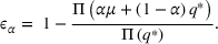
The sensitivity ϵ _40%, for instance, is the fraction of retailer's maximum expected profit that is lost for a mean coefficient of α = 40%. For the wholesale price contract shown in Figure 2b, the sensitivity is ϵ _40% = 1.9%. The flatness of the retailer's expected profit function is not unique to the wholesale price contract but can be observed under many commonly analyzed contracts. Table 1 provides the empirical estimates for the mean coefficient and the sensitivities of commonly analyzed supply contracts.

TABLE 1

Steepness of the decision‐maker's expected profit functions of selected contracts analyzed in the literature

			Contract parameters
			Retail price	Wholesale price	Buyback price	Revenue share		Sensitivity
Contract	Authors	Demand	r	w	b	λ	α	$ε_{40 %}$	$ε_{60 %}$
WPC	Schweitzer and Cachon (2000)	U(1,300)	12	3	–	–	60%	1.8%	4.1%
	Bolton and Katok (2008)	U(0,100)	12	3	–	–	56%	1.9%	4.1%
	Bostian et al. (2008)	U(1,100)	4	1	–	–	36%	1.9%	4.2%
	Bolton et al. (2012)^a	U(1,100)	12	3	–	–	89%	1.9%	4.2%
	Rudi and Drake (2014)^b	N(1000,400²)	12	3	–	–	70%	0.8%	1.8%
BBC	Ren and Croson (2013)	N(100,30²)	10	4	2	–	93%	0.6%	1.3%
	Katok and Wu (2009)	U(0,100)	12	9	8	–	78%	1.9%	4.1%
		U(50,150)	12	9	8	–	37%	0.8%	1.8%
RSC	Katok and Wu (2009)	U(0,100)	12	1	–	1/3	44%	1.9%	4.1%
		U(50,150)	12	1	–	1/3	89%	0.8%	1.8%

Abbreviations: BBC, buyback contract; RSC, revenue‐sharing contract; WPC, wholesale price contract.

Pooled data from managers and students in Phase 2 of the basic treatments.

Data from the uncensored treatment.

Hypotheses

The contracts in Table 1 have low sensitivity, such that deviating from the optimal order quantity has a small effect on expected profit. Under service‐level contracts, low sensitivity can be avoided, such that deviations from the optimal order quantity become costly and the consequences of deviating from optimal order quantities have high salience. From Proposition 1, we know that service‐level contracts generally have steeper expected profit functions than wholesale price contracts, which leads to the following hypothesis: Hypothesis 1.

The average order quantity is closer to the optimal order quantity under a service‐level contract than under the corresponding wholesale price contract.

From Proposition 2, we know that service‐level contracts have more concave expected profit functions than wholesale price contracts do. This result implies that order variability is more costly under a service‐level contract than under the corresponding wholesale price contract. The expected consequences are stated in the following hypothesis: Hypothesis 2.

Orders are less variable under a service‐level contract than under the corresponding wholesale price contract.

The expected behavior stated in Hypotheses 1 and 2 has consequences for the expected supply chain profit, that is, the sum of the expected profits of the supplier and the retailer. The closer average order quantities are to the optimal order quantity, and the less variable they are, the higher the expected supply chain profit is. A standardized measure of expected supply chain profit is supply chain efficiency, that is, the expected supply chain profit achieved divided by the expected supply chain profit from the optimal order quantity, and we hypothesize the following: Hypothesis 3.

Supply chain efficiency is higher under a service‐level contract than under the corresponding wholesale price contract.

The above hypotheses concern performance differences between service‐level contracts and wholesale price contracts. There exists a set of service‐level contracts with different combinations of contract parameters that results in the same optimal order quantity (Figure 1). To achieve a certain optimal order quantity

q^{*}

, service‐level contracts with a low service level s require a higher unit penalty p than service‐level contracts with a high service level s. The contract parameters that result in a given optimal order quantity affect the steepness and concavity of the expected profit function. As we increase the unit penalty cost and decrease the service level to achieve a given optimal order quantity, the steepness and concavity of the expected profit function increase. We expect that service‐level contracts with steep expected profit functions (high unit penalty and low service level) perform better than the corresponding service‐level contracts with flat expected profit functions (low unit penalty and high service levels), and we hypothesize as follows: Hypothesis 4.

The performance of the corresponding service‐level contracts is increasing in the steepness of their expected profit functions. The steeper the contract, the

closer average order quantities are to the optimal order quantity,

lower the variability of orders is, and

the higher the supply chain efficiency is.

MAIN EXPERIMENT

We use laboratory experiments to analyze human decision making under supply contracts. Our main experiment has four treatments, one wholesale price contract treatment serving as a benchmark, and three service‐level contract treatments.

Design

Table 2 provides an overview of the treatments. All treatments used discrete uniformly distributed demand between 1 and 100 and a retail price of r = 12 francs. Ideally, we would use treatments that achieve the optimal order quantities with the same fixed payments and the same maximum expected profits. Unfortunately, this is not feasible, and we need to vary one of the components between treatments. We decided to vary the fixed payments and ensure that ordering the optimal quantities yields the same expected profit of 342 francs in all treatments. Subjects were informed that francs would be converted into cash at an exchange rate of 3000 francs to the dollar at the end of the experiment.

TABLE 2

Treatments used in main laboratory experiment

	Fixed payment	Wholesale price	Retail price	Service level	Penalty cost	Optimal order	Sensitivity		Sample size
Treatment	E	w	r	s	p	q ^*	$ε_{40 %}$	$ε_{60 %}$	N
T1: WPC	–	3	12	–	–	75	1.9%	4.2%	30
T2: SLC_75%,145	225	6	12	75%	145	75	25.8%	61.0%	28
T3: SLC_100%,12	264	6	12	100%	12	75	3.9%	8.4%	30
T4: SLC_75%,6	205	6	12	75%	6	60	0.6%	1.3%	28

Abbreviations: SLC, service‐level contract; WPC, wholesale price contract.

We chose a high‐margin condition such that inventory is optimally stocked above average demand (

q^{*}

> μ) because such contracts are more likely to be observed in practice (Bolton et al., 2012; Katok & Wu, 2009; Wu & Chen, 2014), and service levels below 50% are uncommon in practice (C. M. Chen & Thomas, 2018; Gruen et al., 2002). For the wholesale price contract of Treatment 1, we used a wholesale price of w = 3 francs, resulting in an optimal order quantity of

q^{*}

= 75 units. The wholesale price of the service‐level contracts was w = 6 francs. In Treatment 2, we used the steep service‐level contract, and in Treatment 3, we used the flat service‐level contract (see Figure 1).

Treatments 1 to 3 are sufficient to test our hypotheses. The hypotheses are based on arguments regarding the differences in the steepness of the expected profit functions and do not address the possibility that the stipulated service level might serve as an alternative anchor to average demand. Subjects might anchor on the quantity implied by the stipulated service level times the maximum demand, that is, 75 and 100 for the steep and flat service‐level contracts, respectively. To analyze whether such an anchoring effect exists, we include Treatment 4, in which we use a service‐level contract with the same service level as in Treatment 2 but with a lower unit penalty cost.

Subjects placed orders over 100 periods. Demand was randomly drawn before the experiment and was the same for all subjects and treatments. At the beginning of a period, before demand was revealed, subjects determined their order quantity. They received information about the demand distribution, contract parameters, and retail price. They were also informed that leftover inventory at the end of a period had no value and could be discharged for free. At the end of each period, demand for the period was revealed along with the profit made. The written instructions included examples to illustrate profit calculation. Throughout the sessions, there was no time pressure. The instructions and screenshots are presented in Supporting Informations EC.1 and EC.2, respectively.

Protocol

All sessions were conducted at the Laboratory for Behavioral Operations and Economics at the University of Texas at Dallas and followed the experimental protocol in Figure 3. The experiment was programmed and conducted with the software z‐Tree (Fischbacher, 2007).

FIGURE 3

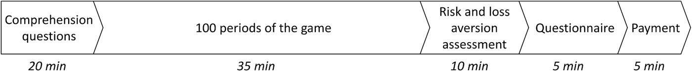
Experimental protocol

Upon entering the laboratory, subjects were randomly assigned to a private computer terminal and given time to read the instructions. After they had read the instructions, subjects could ask questions that were answered privately. During the experiment, communication between subjects was prohibited, and none was observed.

Before the actual experiment started, subjects completed a computerized quiz with 11 (wholesale price contract treatment) or 17 (service‐level contract treatments) questions. The quiz comprised three sections. In the first and second sections of the service‐level contract treatments, subjects had to determine the purchase cost, the number of units sold, the revenue, the service level, the number of units short of the target, the penalty cost, and the profit for two examples that were identical across treatments. In the wholesale price contract treatment, questions regarding the service level, the number of units short of the target, and the penalty cost were excluded. The third section contained general questions about the experiment. The questions and statistics on the answers are provided in Supporting Information EC.3. If all questions of a section were answered correctly on the first attempt, subjects received 1000 francs. If they needed a second attempt, they received 500 francs. If they needed more than two attempts, they did not receive any compensation for the section. Subjects could continue only after they had correctly answered all questions in a section. We used this approach to ensure that subjects had a good understanding of the cost accounting and profit calculation for the particular contract addressed in their treatment.

At the beginning of each period, subjects were reminded of all contract parameters. After each period, they were shown a detailed breakdown of the profit calculation. After the main experiment, all subjects completed two additional tasks (for details, see Supporting Information EC.4). The first task was a computerized version of the risk elicitation task introduced by Holt and Laury (2002). The second task was the computerized loss aversion measurement task of Gächter et al. (2022), which was adapted from an earlier protocol of Fehr and Goette (2007). Subjects earned francs depending on their decisions and the outcome of the risky lotteries.

Finally, subjects answered some general questions, provided demographic data (see Supporting Information EC.5), and were paid, in private, their total individual earnings. The total earnings were based on quiz performance, the profits achieved over the 100 periods of the main experiment, and the two lotteries that we used to elicit subjects’ risk and loss aversion. The sessions lasted approximately 75 min on average. Actual average earnings, including a $5 show‐up fee, were $17.24.

Subjects

A total of 116 subjects participated in six sessions of the experiment. In each session, subjects were randomly assigned to one of the four treatments. Each subject participated in one session, and cash was the only incentive offered. Subjects were students recruited through an online recruitment system from the subject pool of the University of Texas at Dallas.

RESULTS

We first test the hypotheses concerning the higher performance of service‐level contracts, compared to wholesale price contracts. Then, we test the hypotheses concerning the effect of expected profit function steepness on performance, and finally we analyze a potential anchoring effect of the service level.

Unless otherwise stated, we use the Wilcoxon signed‐rank test for one‐sample tests and the Mann–Whitney test for two‐sample tests. All p ‐values we report below are two‐tailed. Summary statistics are provided in Table 3. For the comparisons reported below, we also conducted random effects generalized least squares (GLS) panel regressions, in which we controlled for subjects’ loss aversion or risk aversion. The effect sizes and significance of the contract types are similar to those of the nonparametric tests, and the coefficients for risk and loss aversion are nonsignificant (for details, see Supporting Information EC.6).

TABLE 3

Summary statistics for the main experiment

	T1: WPC	T2: SLC_75%,145	T3: SLC_100%,12	T4: SLC_75%,6
Subjects	30	28	30	28
Normative order quantity	75	75	75	60
Average order quantity	60.16	69.93	61.79	54.37
Within‐subject standard deviation	15.51	8.99	13.88	16.18
Average efficiency	88.15%	97.19%	92.19%	89.19%

Abbreviations: SLC, service‐level contract; WPC, wholesale price contract.

Service‐level contracts versus wholesale price contract

Our first set of analyses compares performance under service‐level contracts with that under a wholesale price contract. The hypotheses state that average order quantities are closer to optimal quantities (Hypothesis 1), that they have lower variability (Hypothesis 2), and that they result in higher supply chain efficiency (Hypothesis 3) under a service‐level contract than under the corresponding wholesale price contract. We first compare the ordering behavior under the wholesale price contract with that under the steep service‐level contract of Treatment 2 and then with that under the flat service‐level contract of Treatment 3. The steep service‐level contract has a 40% sensitivity of 25.8%, which is more than 10 times that of the wholesale price contract; and the flat service‐level contract has a 40% sensitivity of 3.9%, which is approximately twice that of the wholesale price contract (see Table 2).

Average order quantities

Figure 4 depicts the average order quantities per period under (a) the wholesale price contract, (b) the steep service‐level contract, and (c) the flat service‐level contract. Under the steep service‐level contract, average orders are closer to the optimal order quantity than those under the wholesale price contract. The average order quantities are 5.1 units below optimality under the service‐level contract versus 14.8 units under the wholesale price contract. This difference is significant (p < 0.001), which provides support for Hypothesis 1. Under the flat service‐level contract, average order quantities are slightly above the average order quantities under the wholesale price contract, but we do not observe a similar magnitude in the difference from that observed under the steep service‐level contract. Average order quantities are 13.2 units versus 14.8 units below optimality for the flat service‐level contract and the wholesale price contract, respectively. The difference is small (1.6 units) and not significant (p = 0.965).

FIGURE 4

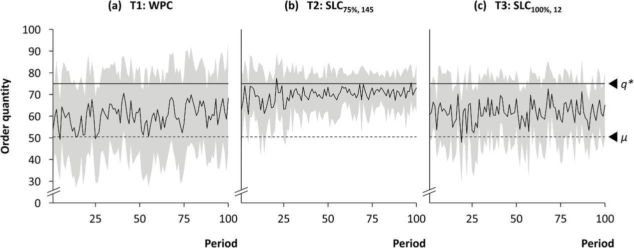
Average order quantities by period under wholesale price contract (WPC) and service‐level contracts (SLC)

Order variability

From Table 3, we see that the within‐subject standard deviation of order quantities under the steep service‐level contract is 8.99 and lower than that under the wholesale price contract (15.51). The difference is significant (t(56) = 4.04, p < 0.001), providing support for Hypothesis 2.

We also observe lower order variability under the flat service‐level contract than under the wholesale price contract. However, the within‐subject standard deviation difference is small and not even marginally significant(t(58) = 0.96, p = 0.342).

Supply chain efficiency

To compute supply chain efficiency, we must specify the unit production cost c of the supplier. In our analyses, we set them equal to the wholesale price in the wholesale price contract, that is, c = w = 3. Then, the supply chain is coordinated under the wholesale price contract. For service‐level contracts, we choose parameter values that result in the same supply chain coordinating optimal order quantity.

Under a wholesale price contract, a self‐interested profit‐maximizing supplier charges a wholesale price w in excess of his or her unit production cost c, and double marginalization causes the retailer to order less than the supply chain optimal order quantity, leading to an efficiency loss. Such an efficiency loss cannot be avoided under a wholesale price contract but can be avoided under a service‐level contract (Sieke et al., 2013). To allow an easier comparison of efficiency losses due to behavioral factors between wholesale price contracts and service‐level contracts, we use in our experiments wholesale price contracts with w = c, such that also the wholesale price contract coordinates the supply chain and choose corresponding service‐level contracts. Then, the optimal order quantities and the optimal expected supply chain profits are the same for all contracts.

The fixed payments under the service‐level contracts can be viewed as a transfer from the supplier to the retailer. Therefore, in the total supply chain profit, the fixed payment cancels out and has no effect on the efficiency result.

Under the steep service‐level contract, supply chain efficiency is 97.2% and is significantly higher than that under the wholesale price contract, 88.1% (p < 0.001), providing support for Hypothesis 3. Under the flat service‐ level contract, supply chain efficiency is 92.2%, which is not significantly higher than that under the wholesale price contract (p = 0.399).

The results of our experiment provide some support for Hypotheses 1–3; that is, all experimental results are in the directions stated in these hypotheses. For the steep service‐level contract, all differences are highly significant (p < 0.001 for all comparisons between the steep service‐level contract and the wholesale price contract). For the flat service‐level contract, the differences are not significant. We conclude that service‐level contracts can outperform wholesale price contracts but that it is important to design a supply contract with a steep expected profit function to realize the performance potential that this contract type offers.

Steep versus flat service‐level contract

The above analyses indicated that the steepness of the expected profit function affects ordering behavior. Hypothesis 4 states the performance differences between steep and flat service‐level contracts with respect to (a) average order quantities, (b) order variability, and (c) supply chain efficiency, and we next formally test this hypothesis.

Average orders under the steep service‐level contract are significantly above those under the flat service‐level contract (p < 0.001), which provides support for Hypothesis 4(a). From Table 3, we see that a steeper expected profit function leads to less order variability among service‐level contracts. The within‐subject standard deviation is significantly lower under the steep than under the flat service‐level contract (t(58) = 3.60, p < 0.001), providing support for Hypothesis 4(b). We also find support for Hypothesis 4(c). Significantly higher efficiency is observed under the steep service‐level contract than under the flat service‐level contract (p < 0.001).

OTHER EXPLANATIONS

We can explain why the steep service‐level contract performs better than the flat service‐level contract and the wholesale price contract by the steepness of the expected profit functions and the resulting salience of the optimal solution. Here, we consider other factors that might explain our results.

Service‐level anchor

If the service level served as an anchor, increasing the service level and maintaining the optimal order quantity would increase the average orders. The comparison of the steep service‐level contract in Treatment 2 with a service level of 75% and the flat service‐level contract in Treatment 3 with a service level of 100% shows that the service‐level contract with the higher service level has smaller average order quantities. However, it has also a flatter expected profit function, and we cannot exclude the possibility that we observed superposed effects: A flatter expected profit function reduces order quantities, and a higher service‐level anchor increases them.

Ideally, we would design a service‐level contract with the same expected profit function and optimal order quantity but with different service levels. Unfortunately, this is not possible. When we vary the service level, we must change the unit penalty (see Figure 1) and thus the expected profit function to maintain the same optimal order quantity. However, we can use the results of Treatment 4 to obtain an indication of whether people anchor on the service level.

In Treatment 4, we used the same service level of 75% as in Treatment 2 but used a unit penalty cost of p = 6 instead of p = 145. The contract of Treatment 4 has a flatter expected profit function than the steep service‐level contract of Treatment 2, and its optimal order quantity is 15 units smaller (60 as opposed to 75 units). If the service level served as an additional anchor, the mean coefficient α should be smaller in Treatment 4 than in Treatment 2. This is because a potential service‐level anchor is above the optimal order quantity in Treatment 4, whereas it is equal to the optimal order quantity in Treatment 2.

In our experiments, we observe the opposite effect. The mean coefficients are α = 56.3% and 20.3% in Treatment 4 and 2, respectively. The difference in the mean coefficient is significant (p = 0.002), providing another indication that the steeper expected profit function, rather than the service‐level anchor, explains behavior under service‐level contracts.

Figure 5 shows the average per period order quantities for Treatments 2 and 4. We observe that they start at approximately the same level and then diverge over 30 periods before they level out. Average order quantities in the first period of the treatments do not significantly differ (average order quantities of 62.6 and 59.5 in Treatments 2 and 4, respectively, p = 0.404). Fitting a random effects GLS regression to the data from the first 30 periods of Treatment 4, we find a significant order decrease of 0.361 units per period (standard error = 0.071, GLS, two‐tailed p < 0.001), which is significantly different from that of Treatment 2 (GLS, two‐tailed p < 0.001), in which we do not observe a significant trend over the first 30 periods (GLS, two‐tailed p = 0.604). The results suggest that subjects might initially anchor on the stipulated service level and then adjust toward their final decision over time.

FIGURE 5

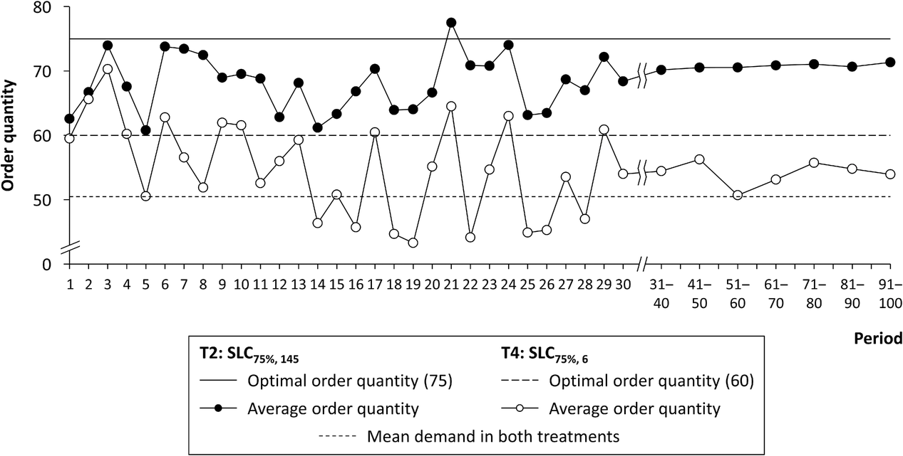
Average order quantities by period in service‐level contract (SLC) Treatments 2 and 4

We note that neither the comparison of Treatments 2 and 3 nor the comparison of Treatments 2 and 4 can exclude the possibility that a service‐level anchoring effect exists that is superposed by the effect that steepness of the expected profit function has on ordering. However, these results indicate that if an anchoring effect existed, it diminished over time, and its effect size would be much smaller than the size of the expected profit function steepness effect.

Quantal choice model

We also analyze whether our results can be explained by a quantal choice model. A quantal choice model predicts orders below the profit‐maximizing quantity for high critical fractiles (Su, 2008) and implies a truncated normal distribution of orders around the mode q* for both the wholesale price contract and the flat service‐level contract. The data reject this specification in two ways. First, for both conditions, the theoretical distribution underpredicts actual orders below q* = 75 and overpredicts actual orders above q*. Second, for both conditions, the mode of actual orders appears lower than the theoretical mode of q*. Formally, Kolmogorov–Smirnov tests reject the hypothesis that order quantities are truncated normally distributed (p < 0.05 for both conditions). As a second check, we examine the consistency of the model's rationality parameter β. The theory puts no formal restrictions on the value of β. That said, two hypotheses suggest themselves: either similar β‐values across treatments or, if one argued that error distributions are affected by steepness, higher irrationality (reflected by higher β‐values) for flat than for steep service‐level contracts. We observe the opposite. Details of both analyses can be found in Appendix B. Our results add to the evidence that random error models do not emulate decision strategies in newsvendor settings (Kremer et al., 2010).

Another potential explanation for our results is loss aversion. We take this up in the next section.

ROBUSTNESS CHECKS

In this section, we report the results of additional experiments that we conducted to analyze the robustness of our findings.

Medium steep service‐level contract

In the main experiment, we analyzed flat and steep service‐level contracts and observed that the flat service‐level contract did not perform significantly better than the corresponding wholesale price contract. The similar performance of the contracts can be explained by the similar steepness of their expected profit functions. If steepness were the performance driver, a service‐level contract with high steepness performs better than the wholesale price contract. We observed high performance under the steep service‐level contract. To analyze whether it takes the steepness of the steep service‐level contract to achieve significant improvements over the wholesale price contract or whether a contract with moderate steepness is sufficient, we conducted an experiment with a medium steep service‐ level contract with a service level of s = 80% and unit penalty of p = 37 (Table 4). The contract has a sensitivity of ϵ _40% = 7.8%, which is twice that of the flat service‐level contract but only 30% of that of the steep service‐level contract.

TABLE 4

Treatments analyzing the performance of wholesale price contract and medium steep service‐level contract

	Fixed payment	Wholesale price	Retail price	Service level	Penalty cost	Optimal order	Sensitivity		Sample size
Treatment	E	w	r	s	p	q ^*	$ε_{40 %}$	$ε_{60 %}$	N
T5: WPC_H	–	3	12	–	–	75	1.9%	4.2%	101
T6: SLC_80%,37	233	6	12	80%	37	75	7.8%	18.0%	100

Abbreviations: SLC, service‐level contract; WPC, wholesale price contract.

To determine an appropriate sample size for the experiment, we conducted a power analysis (G*Power, Faul et al., 2007). The results indicated that a sample size of N = 100 subjects per treatment is required to detect an effect size in the expected order quantities of five units at the 5% level with more than a 95% chance. In Treatment 1 of our main experiment (2), we used a sample size of only N = 30 subjects for the wholesale price contract and had to repeat the wholesale price contract experiment with a larger sample size. In the new experiment, we used N = 201 subjects who were randomly assigned to treatments, which resulted in N = 101 observations for the wholesale price contract and N = 100 observations for the medium steep service‐level contract.

The results of the experiment are shown as gray bars in Figure 6. The average order quantities are 10.0 units below optimality under the medium steep service‐level contract versus 18.2 units under the wholesale price contract. The difference is significant (p < 0.001), which provides support for Hypothesis 1. The within‐subject standard deviation is significantly lower under the medium steep service‐level contract than under the wholesale price contract (t(199) = 4.884, p < 0.001), supporting Hypothesis 2. We also find support for Hypothesis 3. Efficiency is significantly higher under the medium steep service‐level contract than under the wholesale price contract (p < 0.001).

FIGURE 6

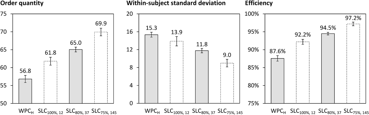
Average order quantity, order variability, and efficiency by treatment. SLC, service‐level contract; WPC, wholesale price contract

Figure 6 also shows the results for the flat service‐level contract (SLC _100% _, ₁₂, Treatment 3) and the steep service‐level contract (SLC _75% _, ₁₄₅, Treatment 2) of the main experiment as white bars. The dashed lines on the white bars indicate that we must be cautious when comparing these results with the results of the wholesale price contract (WPC_H , Treatment 5) and the medium steep service‐level contract (SLC _80% _, ₃₇, Treatment 6) of the new experiment because the sample sizes of Treatments 2 and 3 and Treatments 5 and 6 differ substantially. However, the results match the behavior stated in Hypothesis 4. The contracts shown in Figure 6 are sorted by steepness. As the steepness increases from left to right, average order quantities move toward the optimal order quantity of 75 units, and the order variability decreases and efficiency increases.

Service‐level contract in a low‐margin condition

In the previous experiments, we analyzed high‐margin conditions with optimal order quantities above mean demand. Our model and hypotheses also hold for low‐margin conditions, and we then compare the performance of a wholesale price contract and a service‐level contract with an optimal order quantity of

q^{*}

= 25 units (Table 5).

TABLE 5

Treatments analyzing the performance of wholesale price contracts and service‐level contracts in a low‐profit condition

	Fixed payment	Wholesale price	Retail price	Service level	Penalty cost	Optimal order	Sensitivity		Sample size
Treatment	E	w	r	s	p	q ^*	$ε_{40 %}$	$ε_{60 %}$	N
T7: WPC_L	–	9	12	–	–	25	13.8%	32.3%	76
T8: SLC_25%,48	50	11	12	25%	48	25	65.1%	109.2%	75

Abbreviations: SLC, service‐level contract; WPC, wholesale price contract.

The results of the experiments are summarized in Table 6. Under the service‐level contract, compared to the wholesale price contract, order quantities are lower (p = 0.081 for all periods and p = 0.005 for the last 50 periods) and closer to optimal order quantities, order variability is lower (p = 0.134 for all periods and p < 0.001 for the last 50 periods), and efficiency is higher (p = 0.018 over all periods and p < 0.001 in the last 50 periods), thus supporting Hypotheses 1–3.

TABLE 6

Summary statistics for low‐profit‐margin treatments

	All periods		Last 50 periods
	T7: WPC_L	T8: SLC_25%,48	T7: WPC_L	T8: SLC_25%,48
Subjects	76	75	76	75
Normative order quantity	25	25	25	25
Average order quantity	38.20	35.42	36.93	32.75
Within‐subject standard deviation	13.89	12.58	12.49	8.75
Average efficiency	26.63%	45.52%	34.72%	65.21%

Abbreviations: SLC, service‐level contract; WPC, wholesale price contract.

The effect sizes and significance are lower over all periods than over the last 50 rounds. The differences can be explained by the subjects’ experiences. When the costs associated with ordering too much or too little become transparent, subjects improve their order decisions. Because the service‐level contract is steeper and more concave than the wholesale price contract, the cost effects are stronger under the service‐level contract than under the wholesale price contract, which can explain the faster improvement under the service‐level contract than under the wholesale price contract.

The results of the low‐margin treatment allow us to address another possible explanation for the order behavior treatment effect that it might be due to subject loss aversion (Kahneman & Tversky, 1979; Tversky & Kahneman, 1991). One reason to suspect that this is an important explanatory factor is that a steeper payoff curve creates a larger loss (negative expected profit) domain, which might change ordering behavior. To examine this possibility, we used a standard loss‐averse utility function (e.g., Schweitzer & Cachon, 2000, Section 2.2.4.) and conducted a grid search to determine how the loss factor (the sole parameter of the utility function) affects the expected utility maximizing order quantity.

Figure 7 reports the results. Loss aversion is indicated when the loss factor is greater than 1 (1 is equivalent to expected profit maximization; values that are less than 1, indicate that losses are favorably weighted). For loss factors in the loss aversion range, the expected utility‐maximizing order quantities are equal or higher under the service‐level contract than those under the wholesale price contract. Intuitively, a steeper payoff curve pushes orders higher to avoid the larger loss domain created by the larger penalties in service contracts for both high‐margin and low‐margin conditions. From the graph, we see that the results of the high‐margin experiments are in line with this prediction, but the results of the low‐margin experiments are the opposite of what is predicted: In the low‐margin experiments, the observed average order quantities are lower under the service‐level contract than those under the wholesale price contract—loss aversion predicts that service‐level contract orders should move away orders further from optimal and not closer as we have observed. So loss aversion cannot explain the consistent pattern of more optimal ordering we observe under service‐level contracts as opposed to wholesale price contracts. There may be loss aversion among the subjects, but this does not explain the main treatment effect.

FIGURE 7

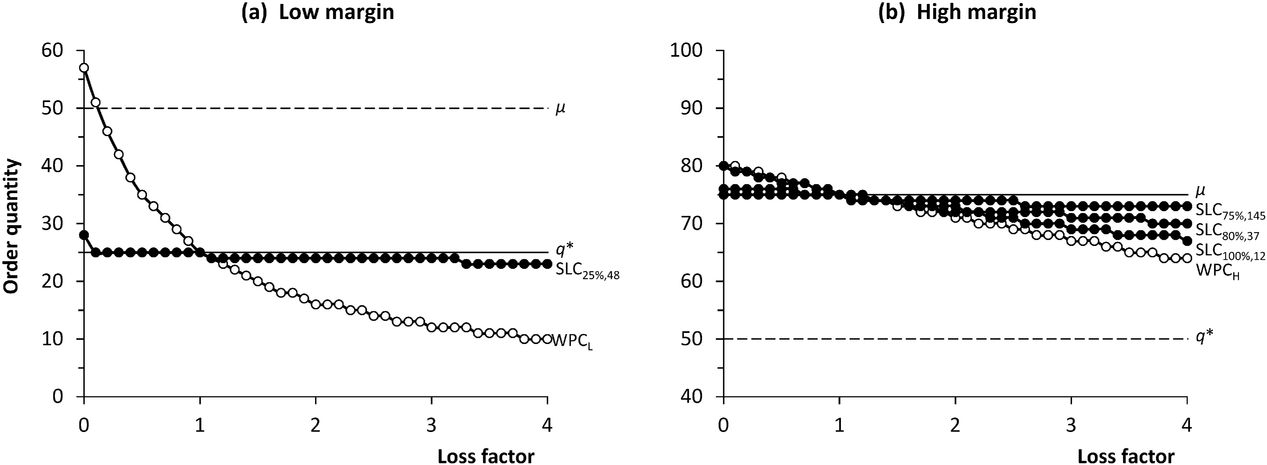
Expected utility‐maximizing order quantity by loss factor. SLC, service‐level contract; WPC, wholesale price contract

Fixed payments in service‐level contracts

We constructed service‐level contracts with endowments of up to 264 francs per round in order to ensure equal profitability across treatments. This enabled us to isolate the effect of salience. However, a large endowment potentially can limit managerial implications. To test that the design implications we draw for the service‐level contracts also hold without substantial endowments, we ran a robustness experiment without per round endowments.

Specifically, we ran the robustness check with two variations of the contract. The first treatment (Treatment 9) was identical to Treatment 2 (Table 2) in the main experiment. The second treatment (Treatment 10) was identical, without the endowment subjects received for each decision round. To account for lower expected profits in the unscaled expected profit function and ensure fair compensation of subjects, they received a large upfront payment of 22,500 francs at the beginning of the experiment, making the payment separate from the order decision task. Other options to equalize profitability, for example, changing the conversion rate or the support of the demand range, would have introduced larger confounds because they change other properties of the expected profit function and hence the underlying decision structure (e.g., a different frequency of losses).

We recruited 54 subjects from the subject pool of the University of Cologne for a laboratory experiment. Subjects were randomly assigned to one of the two treatments. Twenty‐six subjects played the original service‐level contract with E = 225 francs per round (Treatment 9), and 28 subjects received an upfront payment of 22,500 francs instead of 225 francs per round (Treatment 10). A summary of the results can be found in Table 7. In Treatment 9, average orders are 69.64, compared to 69.51 in Treatment 10. The difference is small and not significant (p = 0.5218, Mann–Whitney U‐test). Hence, we can conclude that endowments per round are not significantly affecting order quantities under the steep service‐level contract.

TABLE 7

Summary statistics for the robustness experiment

	T9: SLC_75%,145	T10: SLC_75%,145	T11: WPC	T12: WPC_transf
Subjects	26	28	31	28
Normative order quantity	75	75	75	75
Standard deviation of $π (q^{*}, d)$	297.43	297.43	297.43	2082.00
Average order quantity	69.64	69.51	59.03	59.78
Within‐subject standard deviation	9.30	10.87	15.04	16.47
Average efficiency	97.88%	97.30%	91.28%	90.91%

Abbreviations: SLC, service‐level contract; WPC, wholesale price contract.

Steepness variation in wholesale price contracts

The focus of our analysis and the conclusions concern service‐level contract performance. The question arises whether increasing the steepness of the expected profit function for a wholesale price contract would result in orders that are closer to the optimal order quantity. We cannot increase the steepness similar to service‐level contracts without majorly changing the structure of the contract. A steeper profit function for a wholesale price contract requires to transform the retailers’ profits according to the following form:

π_{t r a n s f} (w, q, d) = A (r \cdot \min (q, d) - w q) - B,

with A and B as constants. Note that for the regular wholesale price contract, A = 1 and B = 0. A is a scaling parameter, where a higher A increases the steepness of the curve. B can be thought of as a large fixed upfront cost. We want to emphasize that due to the upfront cost, such a contract is highly artificial.

While we can pick combinations of A and B that result in the same expected profits for the optimal order quantity, the variability of actual profits for the optimal order quantity increases substantially when we increase the steepness. This is different to the service‐level contract, where a steeper expected profit function would not change the variability of actual profits under the optimal order quantity.

We ran an experiment with two treatments. The first (Treatment 11) replicated the wholesale price contract from Treatment 1 of the main experiment (Table 2). For the second treatment (Treatment 12), we transformed the expected profit function with A = 7 and B = 2051 to ensure sufficient differentiation in steepness. We decided to directly manipulate steepness through the profit function and not through the cash conversion formula as in Ho et al. (2010) since the cash conversion is not very salient in an experimental design with 100 rounds, and it is unclear whether subjects even react to a more complex conversion formula that is applied to their earning at the end of the experiment.

We conducted this experiment online on MTurk due to the intensifying COVID‐19 situation. We recruited 59 participants from the United States. The recruitment was done via Cloudresearch to ensure a good quality of the participants. A summary of the results can be found in Table 7. For the regular wholesale price contract, we observed mean orders of 59.03 and 59.78 for the steep wholesale price contract (p = 0.9094, Mann–Whitney U‐test). An increase in steepness according to the above transformation, hence, does not move order quantities closer to the optimal. The average order quantities between Treatments 11 (average order quantity = 59.03) and Treatment 12 (average order quantity = 59.78) are not significantly different (p = 0.9094, Mann–Whitney U‐test), although the payout function has different steepness.

However, Treatments 11 and 12 do not only differ in steepness, but the steeper wholesale price contract has higher profit variability under the optimal order quantity than the transformed wholesale price contract. With the increased demand risk also comes less valuable feedback from order quantity decisions. This could result in more heuristic behavior like chasing or anchoring. In line with this, we make an observation regarding the ordering behavior of subjects in Treatment 12. Subjects in Treatment 12 under the steep wholesale price contract increase their order quantity from an average of 57.85 units in Periods 1 to 30 to an average of 62.55 units in Periods 31 to 40. In Treatment 11, we observe no such increase. In Period 39, subjects in both treatments incur a randomly drawn demand of two units, resulting in an average loss of 3164 francs per subject in Treatment 12 (subjects who ordered the optimal order quantity of 75 experienced losses of 3458 francs). Subjects in Treatment 11 suffer average losses of just 144 francs. As a reaction to the large loss, subjects in Treatment 12 do not further increase their average order quantities but resort to increased heuristic behavior. This can be seen by comparing order patterns per period across treatments. Similarity in the order pattern between both treatments indicates that subjects adjust to previous demands. We compare the correlation of average orders in both treatments and observe that until period 39 they are only slightly correlated (r = 0.2460). After period 40 the correlation increases to r = 0.4811. This suggests that the underlying increase in profit variability which comes with an increase of steepness in the wholesale price setting mitigates the learning and bears the risk of resorting to heuristics due to the high demand risk.

Taken together, we cannot draw an unambiguous conclusion from the experiment. Steepness can still have an effect on wholesale price contracts; however, we are not able to tease it out due to the underlying changes we made to the decision problem. This is similar to the result of Bolton and Katok (2008) who also found that indirectly increasing the steepness did not have an effect on orders for a wholesale price contract.

DISCUSSION AND MANAGERIAL IMPLICATIONS

We hypothesized that service‐level contracts with a steeper expected profit function improve average order quantities. Our experimental results are in line with this hypothesis. We also argued that the steepness and concavity of the expected profit function of service‐level contracts affect order variability and hypothesized that order variability is lower under steep than under flat profit functions. Our experimental results provided support for the hypothesis. Better average order quantities and lower order variability result in higher efficiency as is made explicit in Figure 8.

FIGURE 8

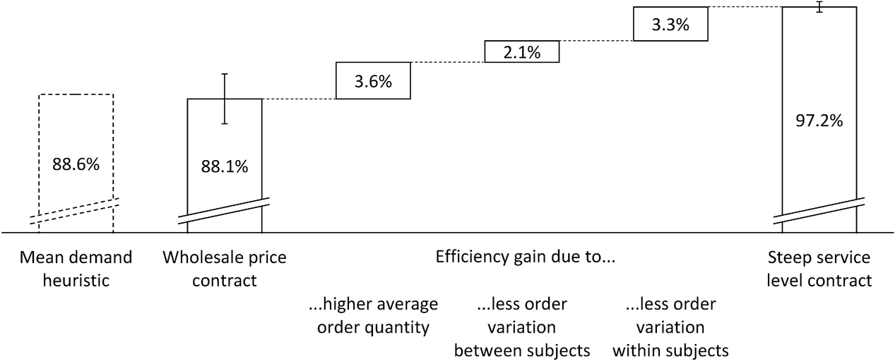
Effect of average order quantities and order variability on supply chain efficiency

The figure shows how the difference in efficiency can be attributed to differences in mean order quantities and variabilities, indicating that both factors play an important role in explaining the efficiency differences that we observed. The first bar shows the efficiency under a mean demand heuristic, whereby the expected demand is ordered in every period. This heuristic can serve as a benchmark and contextualizes the performance that we observed. The second bar shows that performance under the wholesale price contract was lower than that of the mean demand heuristic, albeit not significantly lower. Thus, ordering mean demand in each period would result in a level of efficiency similar to what subjects achieved in the experiment under a wholesale price contract. In both cases, efficiency is more than 11% below optimality. Now observe, from the last bar in the graph that under the steep service‐level contract, the efficiency gap was reduced to less than 3% below optimality. The graph also breaks out the source of the gains in terms of higher average orders and variability both between and within subjects. The important managerial implication here is that ordering under service‐level contracts can be more efficient on average than under wholesale contracts and more reliably efficient both within and between orders.

We analyzed service‐level contracts with a steepness of ϵ _40% = 3.9% (flat), 7.8% (medium steep), and 25.8% (steep) and compared their performance with that of a wholesale price contract with steepness ϵ _40% = 1.9%. The flat service‐level contract achieved an efficiency of 87.6% that was not significantly different from that of the wholesale price contract. The medium steep service‐level contract achieved an efficiency of 92.2%, and the steep service‐level contract an efficiency of 97.2%. The results suggest that service‐level contracts can outperform wholesale price contracts but only if they are sufficiently steep.

Our results have an interesting implication for service‐level contract design. Our results suggest that managers would do well to design service‐level contracts with relatively high penalties, perhaps higher than are currently common. In our study, the service‐level contract that was most successful at eliciting optimal ordering behavior was the one with the highest penalty for missing the agreed‐upon fill rate. We caution against using any simple linear scaling up of the penalty used in our study as a guide to parametrizing field contracts: Unless the decision‐maker has an expected utility function that exhibits extreme diminishing marginal utility, the expected utility loss from raising the penalty by a given percentage in the higher‐stakes environment of the field will have a more substantial effect on salience than the effect we observe in the lab where the stakes were modest. That is, we think it probable that a smaller scaling up in penalty will be sufficient to induce higher salience in the field than in the lab. Field studies would need to be performed to validate this hypothesis.

Our study shows that bounded rationality is less important under service‐level contracts with high salience, as evidenced by the better fit data that show a high degree of fit with the fully rational model we see in Figure 8. That said, investigating the influence of salience on a broader class of contracts is an interesting question and one that will require further investigation. Here, we mention two possible approaches: One approach would be reinforcement adaptive learning models (Bostian et al., 2008; Erev & Roth, 1998) that take salience as a factor in the speed of learning. Another approach would be a quantal choice with additional behavioral restrictions on the error structure (Su, 2008). Suboptimal inventory ordering behavior under wholesale price contracts exhibits a great deal of heterogeneity with regard to the pattern of deviation from optimal (Bolton & Katok, 2008; Moritz et al., 2013). Modeling approaches such as the ones mentioned here could clarify to what extent salience is sufficient to mitigate the various deviations.

We analyze the service‐level contracts with per‐unit penalties. Some service‐level contracts use flat penalties. The literature addresses both types of service‐level contracts (Liang & Atkins, 2013). We have no indication that the flat penalty contract would trigger different behavior than the unit‐penalty contract but validating this would require additional experiments.

Footnotes

1

We screened publicly available service‐level contracts from retails settings on lawinsider.com. Additionally, we had a personal conversation with a practitioner from the telecommunications industry, to get a broader picture on service‐level penalties. The telecommunications company, for example, defines brackets for the magnitude of shortfall of a target service level. For a network service, a 1% shortfall results in a penalty equal to 150% of the monthly payment to the provider. A larger shortfall can lead to penalties in the range of 500% of the monthly payment.

ACKNOWLEDGMENTS

We thank the department editor Mirko Kremer, the senior editor, and two anonymous referees for their constructive comments to improve the paper. This research was funded by the Deutsche Forschungsgemeinschaft (DFG, German Research Foundation) under Germany´s Excellence Strategy–EXC 2126/1–390838866.

Open access funding enabled and organized by Projekt DEAL.

ORCID iD

Sabrina Bonzelet

Ulrich W. Thonemann

APPENDIX A: PROOFS

APPENDIX B: QUANTAL CHOICE MODEL

References

Arrow

K. J.

Harris

Marschak

(1951). Optimal inventory policy. Econometrica, 19(3), 250–272. https://doi.org/10.2307/1906813

Becker‐Peth

Thonemann

U. W.

(2018). Behavioral inventory decisions: The newsvendor and other inventory settings. In Donohue

Katok

Leider

(Eds.), The handbook of behavioral operations (pp. 393–432). Wiley.

Behrenbeck

Diederichs

Großpietsch

Küpper

Leopoldseder

Thonemann

U. W.

(2003). Supply chain champions. The race for service and cost leadership. McKinsey & Company Publication.

Behrenbeck

Küpper

Magnus

K. H.

Großpietsch

Thonemann

U. W.

(2005). Supply chain excellence in retail. McKinsey & Company Publication.

Benzion

Cohen

Peled

Shavit

(2008). Decision‐making and the newsvendor problem. An experimental study. Journal of the Operational Research Society, 59(9), 1281–1287. https://doi.org/10.1057/palgrave.jors.2602470

Bolton

G. E.

Katok

(2008). Learning by doing in the newsvendor problems. A laboratory investigation of the role of experience and feedback. Manufacturing & Service Operations Management, 10(3), 519–538.

Bolton

G. E.

Ockenfels

Thonemann

U. W.

(2012). Managers and students as newsvendors. Management Science, 58(12), 2225–2233. https://doi.org/10.1287/mnsc.1120.1550

Bostian

A. A.

Holt

C. A.

Smith

A. M.

(2008). Newsvendor “pull‐to‐center” effect. Adaptive learning in a laboratory experiment. Manufacturing & Service Operations Management, 10(4), 590–608.

Chen

C. M.

Thomas

D. J.

(2018). Inventory allocation in the presence of service‐level agreements. Production and Operations Management, 27(3), 553–577. https://doi.org/10.1111/poms.12814

10.

Chen

K. Y.

(2018). Buyer‐supplier interactions. In Donohue

Katok

Leider

(Eds.), The handbook of behavioral operations (pp. 459–488). Wiley.

11.

Davis

A. M.

(2015). An experimental investigation of pull contracts in supply chains. Production and Operations Management, 24(2), 325–340. https://doi.org/10.1111/poms.12224

12.

Davis

Reilly

Wilson

(2003). Cost structures and Nash play in repeated Cournot games. Experimental Economics, 6(2), 209–226. https://doi.org/10.1023/A:1025361105730

13.

Erev

Roth

A. E.

(1998). Predicting how people play games: Reinforcement learning in experimental games with unique mixed strategy equilibria. American Economic Review, 88(4), 848–881.

14.

Faul

Erdfelder

Lang

A. G.

Buchner

(2007). G*power 3. A flexible statistical power analysis program for the social, behavioral, and biomedical sciences. Behavioral Research Methods, 39(2), 175–191. https://doi.org/10.3758/BF03193146

15.

Fehr

Goette

(2007). Do workers work more if wages are high? Evidence from a randomized field experiment. American Economic Review, 97(1), 298–317. https://doi.org/10.1257/aer.97.1.298

16.

Fischbacher

(2007). z‐Tree: Zurich toolbox for ready‐made economic experiments. Experimental Economics, 10(2), 171–178. https://doi.org/10.1007/s10683‐006‐9159‐4

17.

Gächter

Johnson

E. J.

Herrmann

(2022). Individual‐level loss aversion in riskless and risky choices. Theory and Decision, 92(3), 599–624. https://doi.org/10.1007/s11238‐021‐09839‐8

18.

Gruen

T. W.

Corsten

D. S.

Bharadwaj

(2002 ). Retail out‐of‐stocks. A worldwide examination of extent, causes and consumer responses . Grocery Manufacturers of America, http://www.uccs.edu/Documents/tgruen/GMA_2002_%20Worldwide_OOS_Study.pdf

19.

Haile

P. A.

Hortacsu

Kosenok

(2008). On the empirical content of quantal response equilibrium. American Economic Review, 98(1), 180–200. https://doi.org/10.1257/aer.98.1.180

20.

Harrison

G. W.

(1989). Theory and misbehavior of first‐price auctions. American Economic Review, 79(4), 749–762.

21.

T. H.

Lim

Cui

T. H.

(2010). Reference dependence in multilocation newsvendor models. A structural analysis. Management Science, 56(11), 1891–1910. https://doi.org/10.1287/mnsc.1100.1225

22.

Holt

C. A.

Laury

S. K.

(2002). Risk aversion and incentive effects. American Economic Review, 92(5), 1644–1655. https://doi.org/10.1257/000282802762024700

23.

Hyndman

Embrey

(2019). Econometrics for experiments. In Donohue

Katok

Leider

(Eds.), The handbook of behavioral operations (pp. 35–88). Wiley.

24.

Kahneman

Tversky

(1979). Prospect theory. An analysis of decision under risk. Econometrica, 47(2), 263–292. https://doi.org/10.2307/1914185

25.

Katok

Thomas

D. J.

Davis

A. M.

(2008). Inventory service‐level agreements as coordination mechanisms. The effect of review periods. Manufacturing & Service Operations Management, 10(4), 609–624.

26.

Katok

D. Y.

(2009). Contracting in supply chains. A laboratory investigation. Management Science, 55(12), 1953–1968. https://doi.org/10.1287/mnsc.1090.1089

27.

Kremer

Minner

vanWassenhove

L. N.

(2010). Do random errors explain newsvendor behavior? Manufacturing & Service Operations Management, 12(4), 673–681.

28.

Liang

Atkins

(2013). Designing service level agreements for inventory management. Production and Operations Management, 22(5), 1103–1117.

29.

Moritz

B. B.

Hill

A. V.

Donohue

K. L.

(2013). Individual differences in the newsvendor problem: Behavior and cognitive reflection. Journal of Operations Management, 31(1‐2), 72–85. https://doi.org/10.1016/j.jom.2012.11.006

30.

Mostberger

(2006). Supply chain controlling: Basis für gemeinsamen Erfolg (in German). Global Supply Chain Summit, 2006, Montreux, Switzerland.

31.

Potters

Suetens

(2020). Optimization incentives in dilemma games with strategic complementarity. European Economic Review, 127, 103453. https://doi.org/10.1016/j.euroecorev.2020.103453

32.

Ren

Croson

R. T. A

(2013). Overconfidence in newsvendor orders. An experimental study. Management Science, 59(11), 2502–2517. https://doi.org/10.1287/mnsc.2013.1715

33.

Romeo

C. J.

Sopher

(1999). Learning and decision costs in one person games. Journal of Applied Econometrics, 14(4), 335–357. https://doi.org/10.1002/(SICI)1099‐1255(199907/08)14:4%3c335::AID‐JAE537%3e3.0.CO;2‐D

34.

Rosling

(2002). Inventory cost rate functions with nonlinear shortage costs. Operations Research, 50(6), 1007–1017. https://doi.org/10.1287/opre.50.6.1007.346

35.

Rudi

Drake

(2014). Observation bias. The impact of demand censoring on newsvendor level and adjustment behavior. Management Science, 60(5), 1334–1345. https://doi.org/10.1287/mnsc.2013.1825

36.

Schweitzer

M. E.

Cachon

G. P.

(2000). Decision bias in the newsvendor problem with a known demand distribution. Experimental evidence. Management Science, 46(3), 404–420. https://doi.org/10.1287/mnsc.46.3.404.12070

37.

Sieke

M. A.

Seifert

R. W.

Thonemann

U. W.

(2013). Designing service level contracts for supply chain coordination. Production and Operations Management, 21(4), 698–714. https://doi.org/10.1111/j.1937‐5956.2011.01301.x

38.

(2008). Bounded rationality in newsvendor models. Manufacturing & Service Operations Management, 10(4), 566–589.

39.

Tversky

Kahneman

(1991). Loss aversion in riskless choice: A reference‐dependent model. Quarterly Journal of Economics, 106(4), 1039–1061. https://doi.org/10.2307/2937956

40.

D. Y.

Chen

K. Y.

(2014). Supply chain contract design. Impact of bounded rationality and individual heterogeneity. Production and Operations Management, 23(2), 253–268. https://doi.org/10.1111/poms.12057

Supplementary Material

Please find the following supplemental material available below.

For Open Access articles published under a Creative Commons License, all supplemental material carries the same license as the article it is associated with.

For non-Open Access articles published, all supplemental material carries a non-exclusive license, and permission requests for re-use of supplemental material or any part of supplemental material shall be sent directly to the copyright owner as specified in the copyright notice associated with the article.

0.00 MB

1.74 MB

Decision making under service‐level contracts: The role of cost saliency

Abstract

Keywords

INTRODUCTION

THEORETICAL ANALYSIS OF THE SERVICE‐LEVEL CONTRACT

DEVELOPMENT OF HYPOTHESES

Salience of optimal order quantity

Mean coefficient and profit sensitivity

Hypotheses

MAIN EXPERIMENT

Design

Protocol

Subjects

RESULTS

Service‐level contracts versus wholesale price contract

Average order quantities

Order variability

Supply chain efficiency

Steep versus flat service‐level contract

OTHER EXPLANATIONS

Service‐level anchor

Quantal choice model

ROBUSTNESS CHECKS

Medium steep service‐level contract

Service‐level contract in a low‐margin condition

Fixed payments in service‐level contracts

Steepness variation in wholesale price contracts

DISCUSSION AND MANAGERIAL IMPLICATIONS

Footnotes

1

ACKNOWLEDGMENTS

ORCID iD

APPENDIX A: PROOFS

APPENDIX B: QUANTAL CHOICE MODEL

References

Supplementary Material