Sage Journals: Discover world-class research

Abstract

Human decision making in the newsvendor context has been analyzed intensively in laboratory experiments, where various decision biases have been identified. However, it is unclear whether the biases also exist in practice. We analyze the ordering decisions of a manufacturer who faces a multiproduct newsvendor problem with an aggregate service‐level constraint. We find that the manufacturer broadly exhibits the same biases as subjects in the laboratory and is prone to another bias that has not been identified before, that is, group aggregation. The bias can be attributed to the multi‐product problem of the manufacturer, and refers to the observation that the service levels are not optimized for individual products, but rather for product groups. Our data allow us to analyze the performance of a manufacturer in detail and we find that target service levels are achieved effectively, but not efficiently. We provide rationales for the manufacturer's ordering behavior, discuss managerial implications, and quantify the financial benefits of debiasing ordering decisions.

Author Video

Keywords

behavioral operations decision analysis empirical decision making multiproduct newsvendor service‐level contract

INTRODUCTION

The newsvendor problem is one of the fundamental problems in operations management. The basic model considers a decision maker who is facing stochastic demand for a perishable product and must decide how much of the product to order to maximize expected profit. The model was introduced by Edgeworth (1888) and many variations and extensions of the model have been developed (Choi, 2012).

In their seminal behavioral operations paper, Schweitzer and Cachon (2000) analyzed ordering decisions of human decision makers in a newsvendor setting. They conducted experiments and found that orders deviated from the normative predictions of the newsvendor model. The subjects overreacted to recent demand realizations and their average order quantities were pulled toward the mean demand. The biases are robust and have been observed under different demand distributions (Benzion et al., 2008), with different subject pools (Bolton et al., 2012; Lee et al., 2018; Moritz et al., 2013), under various framings (Katok & Wu, 2009; Kremer et al., 2010), and are stable over time (Bolton & Katok, 2008; Lurie & Swaminathan, 2009; Ockenfels & Selten, 2015). The common explanations of the biases are demand chasing (Bolton & Katok, 2008; Lau & Bearden, 2013), anchoring (Bostian et al., 2008), and inventory error minimization (Ho et al., 2010; Kremer et al., 2014). For a comprehensive review on behavioral inventory papers, we refer to Becker‐Peth and Thonemann (2018).

There exist rich bodies of literature on normative newsvendor models and newsvendor laboratory experiments, but the ordering behavior of actual decision makers in a newsvendor environment has not been analyzed. We take a first step toward filling this gap. In this paper, we analyze the orders of a manufacturer who distributes bakery products via the stores of one of Europe's largest retailers. The problem that the manufacturer faces is a newsvendor‐type problem: Demand is uncertain, products are perishable, and the products' shelf life and selling period are one day without replenishment during the day. However, unlike in the standard newsvendor model, the manufacturer does not face an unconstrained optimization problem, but must ensure a minimum service level. More precisely, the manufacturer has to ensure that a certain fraction of the products is in stock at the end of the day, that is, he must achieve an aggregated target service level.

The newsvendor problem with the specific aggregate service‐level constraint that the manufacturer faces has not been analyzed before in the literature. We analytically derive the optimal ordering decision for the problem. In the optimal solution, service levels are differentiated across products based on the demand uncertainties, unit revenues, and unit costs of products. We compare the actual order quantities with the optimal quantities and find that the manufacturer's ordering decisions are effective, but not efficient. The manufacturer achieves the aggregated target service level generally, but at costs well above the optimal cost. The efficiency gap can be attributed to three effects: behavioral forecasting, inventory error minimization, and group aggregation. The first two effects were identified in previous laboratory experiments and we find empirical evidence for them in the order data of the manufacturer. The third effect, group aggregation, has not been identified before. It refers to the observation that service levels are differentiated per product groups, but not per individual product. This approach simplifies the task but harms efficiency.

Our results have important implications for behavioral operations management research. Research in this area has relied on analytical models and laboratory experiments, and the behavioral operations management community has discussed extensively how well the results of laboratory experiments translate into practice. We analyze the inventory decisions of an actual manufacturer in a newsvendor environment and show that the biases that have been identified in the laboratory also exist in practice.

Our results are of interest not only to researchers but also to practitioners. We quantify the magnitude of the financial benefits of eliminating decision biases by comparing the manufacturer's performance with the performance that the manufacturer would have achieved if he had implemented an unbiased solution. The results show that eliminating behavioral biases increases the operating profit substantially.

ANALYTICAL MODEL

The manufacturer that we analyze in this paper distributes

N

products via multiple stores of a retailer. For each unit of product

i

that is sold at the retailer, the manufacturer receives a unit revenue of

r_{i}

. The unit cost of product

i

c_{i}

and leftover inventory has negligible salvage value. Excess demand is lost. The manufacturer must decide how many units of each product to deliver to each store. We refer to this quantity as order quantity.

Depending on the contribution margins of the products, the expected profit maximizing orders can result in lower service levels than the retailer requires. To avoid low availability of products at the end of a day, the retailer requires that the manufacturer achieves a service level per store of at least

\bar{α}

. The retailer uses a Type‐I service level that measures the average fraction of products available at the end of the day. The manufacturer can vary the service levels among the products, but an average service level of at least

\bar{α}

across all products must be achieved at each store. This means that on average,

\bar{α}

percent of the products must be available in each store. The manufacturer has agreed to achieve the target service level, but the consequences of falling short of it have not been formally specified. However, there exists a mutual understanding between the manufacturer and the retailer that the business relationship is sustainable only if the target service level is generally achieved. For our model, we assume that the manufacturer's objective is maximizing expected profit under the constraint that the aggregated target service level is achieved.

The manufacturer's optimization problem can be solved for each store individually and we next consider a single store. The solution to the optimization problem takes place in two stages. First, the manufacturer estimates the demand distribution for each product and then solves a multiproduct newsvendor problem.

Demand forecasting

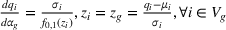
We denote the demand for product

i

in period

t

Y_{i, t}

. We consider normally distributed demand with mean

μ_{i, t}

and standard deviation

σ_{i, t}

, that is independent between products and stores.

In retail environments like the one that we consider, demand is typically autocorrelated (van Donselaar et al., 2010). It can be modeled as an ARIMA(0,1,1) time series, for which single exponential smoothing is the mean squared error minimizing forecasting method (Chatfield, 2001), and we use this approach in our model.

The manufacturer receives censored demand information, that is, he does not observe demands

y_{i, t}

but observes sales

s_{i, t} = \min {y_{i, t}, q_{i, t}}

at the end of period

t

. Demands that exceed the order quantity

q_{i, t}

must be estimated. A standard approach is to estimate demands based on sales by (Bell, 1981; Wecker, 1978)

\begin{matrix} {\hat{y}}_{i, t} = \{\begin{matrix} s_{i, t} & if s_{i, t} < q_{i, t} \\ E (Y_{i, t} | y_{i, t} \geq q_{i, t}) & if s_{i, t} = q_{i, t} . \end{matrix} \end{matrix}

If sales are below the order quantity (

s_{i, t} < q_{i, t}

), then the demand is uncensored and equal to sales. If sales are equal to the order quantity (

s_{i, t} = q_{i, t}

), then the demand is at least as high as the order quantity and is estimated by the conditional expectation

E (Y_{i, t} | y_{i, t} \geq q_{i, t}) = \int_{q_{i, t}}^{\infty} x {\hat{f}}_{i, t} (x) d x / \int_{q_{i, t}}^{\infty} {\hat{f}}_{i, t} (x) d x

, where

{\hat{f}}_{i, t} (x)

is the estimate of the density function of the demand for product

i

in period

t

Based on the estimate of the demand of the previous period,

{\hat{y}}_{i, t}

, and the demand forecast of the previous period,

{\hat{μ}}_{i, t}

, the expected demand of the following period is estimated using exponential smoothing as

{\hat{μ}}_{i, t + 1} = η {\hat{y}}_{i, t} + (1 - η) {\hat{μ}}_{i, t},

where

η

denotes the smoothing factor.

The variance

{\hat{σ}}_{i, t + 1}^{2}

of the demand distribution is estimated based on the average squared forecast error. The density function of the demand of product

i

for period

t + 1

{\hat{f}}_{i, t + 1} (y)

is a normal distribution with mean

{\hat{μ}}_{i, t + 1}

and standard deviation

{\hat{σ}}_{i, t + 1}

. We denote the corresponding distribution function by

{\hat{F}}_{i, t + 1} (y)

We neglect demand substitution effects, which seems reasonable in the setting that we analyze. In our application, substitution rates are small and the impact on the resulting order quantities and profits is negligible. We evaluated the effect of substitution on the manufacturer's profit and found that order quantities differ by 1.1% on average and the realized profit would be 0.6% higher than the optimal solution without substitution. To keep the following models analytically tractable and the behavioral analyses technically feasible, we disregard substitution effects in the model.

Newsvendor system approach

The manufacturer's objective is to maximize expected profit, subject to a constraint on the service level. The probability that product

i

is available at the end of a period is

{\hat{F}}_{i} (q_{i})

. The optimization problem can be decomposed by day and we have dropped subscript

t

for notational convenience. The average service level at the store is

\frac{1}{N} \sum_{i = 1}^{N} {\hat{F}}_{i} (q_{i})

and must be at least

\bar{α}

The optimization problem is

Z^{*} = \max_{q_{1}, …, q_{N}} \sum_{i = 1}^{N} \int_{y_{i}} (r_{i} \min (q_{i}, y_{i}) - c_{i} q_{i}) {\hat{f}}_{i} (y_{i}) d y_{i}

s.t. \frac{1}{N} \sum_{i = 1}^{N} {\hat{F}}_{i} (q_{i}) \geq \bar{α},

q_{i} \geq 0 .

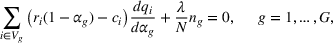
If Constraint (4) is not binding, optimal order quantities are determined for each product individually by the standard newsvendor formula, that is,

q_{i}^{*} = {\hat{F}}_{i}^{- 1} (\frac{r_{i} - c_{i}}{r_{i}})

. Then, the service level of product

i

is equal to its critical ratio

C R_{i} = \frac{r_{i} - c_{i}}{r_{i}}

. If the service level constraint is binding, the following theorems hold. The optimality conditions are stated in Theorem 1. The proof is contained in Appendix A. Theorem 1

The optimal order quantities fulfill the following conditions:

\begin{matrix} \frac{c_{i} {\hat{F}}_{i} (q_{i}^{*}) - (r_{i} - c_{i}) (1 - {\hat{F}}_{i} (q_{i}^{*}))}{{\hat{f}}_{i} (q_{i}^{*})} \\ = \frac{c_{j} {\hat{F}}_{j} (q_{j}^{*}) - (r_{j} - c_{j}) (1 - {\hat{F}}_{j} (q_{j}^{*}))}{{\hat{f}}_{j} (q_{j}^{*})} i, j = 1, …, N . \end{matrix}

The theorem states the optimality conditions in terms of the order quantities. Some of our analyses will be based on service levels. For such analyses, it is more convenient to use the service‐level definition

α_{i}^{*} = {\hat{F}}_{i} (q_{i}^{*}

) and rewrite Equation (6) as

\frac{r_{i} α_{i}^{*} - r_{i} + c_{i}}{\frac{1}{\hat{σ_{i}}} f (z (α_{i}^{*}))} = \frac{r_{j} α_{j}^{*} - r_{j} + c_{j}}{\frac{1}{\hat{σ_{j}}} f (z (α_{j}^{*}))} i, j = 1, …, N,

where

f (\cdot)

denotes the density function of a standard normal distribution and

z (α) = F^{- 1} (α)

the z‐value of the inverse cumulative standard normal distribution function.

The optimality conditions have an intuitive interpretation. The numerator is the expected cost increase of a marginal order quantity increase in product

i

, that is,

d Z / d q_{i} = r_{i} α_{i}^{*} - r_{i} + c_{i}

. The denominator is the expected service‐level increase of a marginal order quantity increase, that is,

d α_{i} / d q_{i} = 1 / \hat{σ_{i}} f (z (α_{i}^{*}))

. The ratio of both is the expected cost increase of a marginal service‐level increase and the optimality condition requires it to be the same for all products.

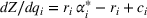
In the optimal solution, the service levels are differentiated based on the characteristics of the products and the demand, which is formally stated in Theorem 2. Theorem 2

The optimal service level

α_{i}^{*}

of product

i

(a)

increases in the unit revenue

r_{i}

;

(b)

decreases in the unit cost

c_{i}

; and

(c)

decreases in the standard deviation of the demand

σ_{i}

BEHAVIORAL MODELS

The planning task consists of two subtasks, demand forecasting and inventory optimization. Literature has identified several decision biases for these subtasks that might be relevant in our setting. For behavioral forecasting, we will analyze system neglect behavior and for behavioral inventory management, we will look at group aggregation, anchoring, and inventory error minimization.

Behavioral demand forecasting

Behavioral operations management literature suggests that actual ordering decisions are more than optimally adjusted toward recent demand realizations, an effect referred to as demand chasing (for instance, Bolton & Katok, 2008; Bostian et al., 2008; Schweitzer & Cachon, 2000). Other studies with stationary demand forecasts focus on how subjects sample historical data to estimate future demand (Tong & Feiler, 2017). They find that subjects naively sample too few observations from historical data to estimate the mean point forecast. Another study on stationary demand forecasts analyzes how censored demand settings impact the estimate of point forecasts (Feiler et al., 2013). They find that subjects show a censorship bias, that is, they underestimate the extent of unobserved lost sales and “rely too heavily on the observed censored sample” (Feiler et al., 2013). For a comprehensive review on studies in behavioral forecasting, see Goodwin et al. (2018).

Focusing on demand series forecasting, Kremer et al. (2011) analyze how subjects forecast autocorrelated time series similar to ours. They found that subjects' forecasting behavior in correlated demand environments is consistent with the mechanics of a single exponential smoothing forecast. However, subjects overadjust in settings where they should not adjust (corresponding to small

η

) and underadjust in settings where they should adjust (high

η

). In our setting, we also have autocorrelated demand and we will use their approach.

Based on their findings, we model forecasting as

μ_{i, t + 1}^{B} = b η_{i, t} {\hat{y}}_{i, t} + (1 - b η_{i, t}) μ_{i, t}^{B},

where

μ_{i, t + 1}^{B}

denotes the behavioral forecast of the demand of product

i

in period

t + 1

. The mean squared error minimizing smoothing factor

η_{i, t}

is determined per product and weekday and is updated each period. The only difference between Equation (8) and the forecasting model of our analytical model (Equation 2) is the behavioral forecasting factor

b

. For a behavioral forecasting factor of 1, there exists no forecasting bias and the models are identical. A behavioral forecasting factor

b > 1

indicates overreaction to recent demand realizations and a factor

b < 1

indicates underreaction (Kremer et al., 2011). Such modeling is parsimonious while describing human behavior quite well (Goodwin et al., 2018). We refer to the model taking behavioral forecasting into account as Model 1 in our subsequent analysis.

Behavioral inventory optimization

Based on the demand forecasts, the order quantities are optimized. In an optimal solution, the order quantities are chosen, such that the target service level is reached and expected profits are maximized. The service levels then depend on the demand uncertainties, unit revenues, and unit costs of the products (Theorem 2). However, literature on behavioral inventory management suggests various deviations from expected profit maximizing behavior. Prominent observations include anchoring (Bolton & Katok, 2008) and ex post inventory error minimization (Kremer et al., 2014). Before we look at these factors, we will introduce a factor that is specific to our setting, we refer to this as group aggregation.

Group aggregation

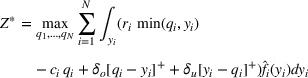
In our setting, the manufacturer must optimize service levels for 23 products. This is analytically challenging. A potential simplification would be to split the products into

G

different groups and optimize the service level per group

g = 1, …, G

. Each group then consists of a set of products

V_{g}

. The number of products,

n_{g}

, in a group may vary between groups. The decision variable is then

α_{g}

as the service level for each product in a group.

The optimization problem of the manufacturer can be formulated as follows:

\max \sum_{g = 1}^{G} \sum_{i \in V_{g}} ((r_{i} - c_{i}) q_{i} - r_{i} \int_{0}^{q_{i}} F_{i} (x) d x)

s.t. \frac{1}{N} \sum_{g = 1}^{G} n_{g} α_{g} = \bar{α}

{\hat{F}}_{i} (q_{i}) = α_{g}, \forall i \in V_{g} .

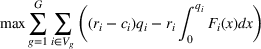
This results in the following optimality condition:

\begin{matrix} \sum_{i \in V_{g}} (r_{i} (1 - α_{g}) - c_{i}) \frac{d q_{i}}{d α_{g}} + \frac{λ}{N} n_{g} = 0, g = 1, …, G, \end{matrix}

with

\frac{d q_{i}}{d α_{g}} = \frac{σ_{i}}{f_{0, 1} (z_{i})}, z_{i} = z_{g} = \frac{q_{i} - μ_{i}}{σ_{i}}, \forall i \in V_{g}

Such a model can be seen as a kind of heuristic for the decision maker. Using aggregated product groups leads to similar target service levels within a group. This results in less than optimal within‐group differentiation compared to optimal individual product‐based differentiation. The actual target service levels of the groups and between groups depend on the group composition. We will refer to the model with group aggregation as Model 2.

Anchoring

Tversky and Kahneman (1974) observed that people who solve a decision task often start with an initial solution that is based on simple features and then adjust the solution toward the optimal solution. Because the final solution is often anchored on the initial solution and not adjusted all the way toward the optimal solution, the heuristic is referred to as the anchoring and insufficient adjustment heuristic.

The anchoring and insufficient adjustment heuristic has been used to explain ordering decisions in the newsvendor problem. A natural anchor in the expected cost minimization models that have been used in the literature is mean demand (e.g., Bolton & Katok, 2008; Bostian et al., 2008; Schweitzer & Cachon, 2000). However, unlike the newsvendor problems considered in previous behavioral research, the problem we consider has a service‐level constraint. The retailer regularly communicates the target service level to the manufacturer and informs him if he misses the target. Therefore, the target service level is a candidate for a natural anchor for the manufacturer's ordering decisions.

We model anchoring using an approach similar to that of Bostian et al. (2008) and introduce an anchoring factor

a

0 \leq a \leq 1

. While Bostian et al. (2008) model anchoring on mean demand, we use the target service level

\bar{α}

as an anchor:

\begin{matrix} q_{i, t} = a {\hat{F}}_{i, t}^{- 1} (\bar{α}) + (1 - a) {\hat{F}}_{i, t}^{- 1} (α_{i}^{*}) = a q_{i, t}^{\bar{α}} + (1 - a) q_{i, t}^{*} . \end{matrix}

Under the anchoring model, the manufacturer first determines the order quantity of product

i

that results in a service level of

\bar{α}

, that is,

q_{i, t}^{\bar{α}} = {\hat{F}}_{i, t}^{- 1} (\bar{α})

and then adjusts the order quantity toward the optimal solution

q_{i, t}^{*} = {\hat{F}}_{i, t}^{- 1} (α_{i}^{*})

. The order quantity is a weighted average of the anchor and the optimal quantity, with weights

a

and

(1 - a)

, respectively. Setting

a = 1

(i.e., full anchoring) leads to a service level of

\bar{α}

for each product. This means that there is no differentiation between products. A weight

a = 0

leads to optimally differentiated service levels.

As a result, we conclude that increasing the anchoring factor

(a)

leads to product service levels that are pulled toward the aggregated target

\bar{α}

. This decreases differentiation between products. Consequently, the anchoring and insufficient adjustment heuristic results in service levels that are between the optimal service levels and the target service level. We will refer to this model as Model 3. The anchoring heuristic can also be used in addition to the group aggregation model. In this case, the manufacturer does not determine optimal service levels for each product, but for each product group and adjusts toward this group‐specific solution. Technically, the manufacturer uses

{\hat{F}}_{i, t}^{- 1} (α_{g}^{*})

in Equation (13) instead of

{\hat{F}}_{i, t}^{- 1} (α_{i}^{*})

, and we will refer to this model as Model 4.

Inventory error minimization

The behavioral operations management literature has suggested inventory error preferences as a potential explanation for ordering behavior (Kremer et al., 2010, 2014). Ho et al. (2010) argue that psychological costs are associated with leftovers and stockouts and that the psychological aversion to leftovers is greater than the disutility for stockouts. This model is a generalization of the model used by Schweitzer and Cachon (2000), where the psychological underage and overage costs are the same.

We use a similar model as Ho et al. (2010) to analyze whether inventory error minimization can explain the manufacturer's ordering behavior. We denote the psychological cost associated with a unit of leftover inventory by

δ_{o}

and the psychological cost associated with a unit stockout by

δ_{u}

. The psychological costs are added to the monetary underage costs (

c_{i}^{u} = r_{i} - c_{i}

) and overage costs (

c_{i}^{o} = c_{i}

). The optimization model is

\begin{matrix} Z^{*} & = & \max_{q_{1}, …, q_{N}} \sum_{i = 1}^{N} \int_{y_{i}} (r_{i} \min (q_{i}, y_{i}) \\ - c_{i} q_{i} + δ_{o} {[q_{i} - y_{i}]}^{+} + δ_{u} {[y_{i} - q_{i}]}^{+}) {\hat{f}}_{i} (y_{i}) d y_{i} \end{matrix}

s.t. \frac{1}{N} \sum_{i = 1}^{N} {\hat{F}}_{i} (q_{i}) \geq \bar{α},

q_{i} \geq 0 .

The objective function corresponds to the objective function of the base model (3) but with adapted over‐ and underage costs. The optimality conditions are

\begin{matrix} \frac{(c_{i}^{o} + δ_{o}) {\hat{F}}_{i} (q_{i}) - (c_{i}^{u} + δ_{u}) (1 - {\hat{F}}_{i} (q_{i}))}{{\hat{f}}_{i} (q_{i})} \\ = \frac{(c_{j}^{o} + δ_{o}) {\hat{F}}_{j} (q_{j}) - (c_{j}^{u} + δ_{u}) (1 - {\hat{F}}_{j} (q_{j}))}{{\hat{f}}_{j} (q_{j})} \forall i, j \end{matrix}

and we will refer to the model as Model 5.

The model of Ho et al. (2010) has no service‐level constraint and inventory error minimization pulls orders toward the mean demand. In our setting, service‐level differentiation in the optimal solution is (besides demand uncertainty) driven by differences in unit revenues and unit costs of the product, and thus by differences in the underage and overage costs. To analyze the impact of psychological costs in our setting, it is important to consider that critical ratios, which include psychological underage and overage costs, vary less between products than critical ratios, which do not include the psychological costs. Assuming the same demand variance between products, this results in more similar target service levels between products. Because of the aggregated service‐level constraint, this results in service levels that are pulled toward aggregated target service level

\bar{α}

. We can again combine the model with the group aggregation model described before and refer to the resulting model as Model 6.

Table 1 summarizes the behavioral models that we will test, and we will use the normative solution of Section 2.2 as a benchmark. Model 1 adds the first decision bias and considers behavioral forecasting, but optimal approaches for determining order quantities. As we will demonstrate, behavioral forecasting improves the model fit considerably, so we use it in all behavioral models. Models 2, 3, and 5 each add an inventory optimization bias to Model 1. Model 2 adds group aggregation, Model 3 adds anchoring, and Model 5 adds inventory error minimization. These models allow us to analyze the significance of individual optimization biases and their effects on the model fits. In Models 4 and 6, we analyze combinations of the biases. Model 4 uses group aggregation and anchoring and Model 6 uses group aggregation and inventory error minimization. Anchoring and inventory error minimization offer alternative explanations for ordering behavior. Because it is unclear how models that contain both decision biases can be interpreted, we do not analyze them.

TABLE 1

Overview of behavioral models analyzed

Decision biases	Model 1	Model 2	Model 3	Model 4	Model 5	Model 6
Behavioral forecasting	$✓$	$✓$	$✓$	$✓$	$✓$	$✓$
Group aggregation		$✓$		$✓$		$✓$
Anchoring			$✓$	$✓$
Inventory error minimization					$✓$	$✓$

To summarize, we will analyze four behavioral factors. (1) Behavioral forecasting: We expect decision makers to put too much weight on recent demand realizations. This will result in biased forecasts that will have a lower forecast accuracy and performance. (2) Group aggregation: Simplifying tasks by not optimizing 23 different service levels, but grouping products together will lead to product clusters that have similar service levels. Service levels will differ between groups, but within‐group differentiation will be small. (3) Anchoring: In our setting, the decision makers need to ensure a certain target service level. Therefore, anchoring on mean demand is not feasible because it would lead to too low service levels. However, we expect decision makers to anchor on the overall target service level. That would lead to too little differentiation between products with all products being pulled‐to‐target. (4) Inventory error minimization: Similar to other behavioral newsvendor studies, this factor is an alternative explanation for the expected pull‐to‐target effect. Adjusting actual cost by adding psychological costs reduces differences in product costs and, consequently, results in more similar target service levels.

EMPIRICAL DECISION ANALYSIS

After developing the analytical and behavioral models, we are analyzing empirical decisions of the manufacturer in this section. We first describe the details of the case and then analyze the service level achieved per store and per product to see if the results are in line with the analytical model. Then, we analyze the behavioral models and their predictions and test which biases can be observed with the empirical newsvendor.

Setting and data

The manufacturer has a product portfolio with 23 bakery items (breads, buns, rolls, pastries, etc.) that are sold at 66 stores of a retailer. The products have a shelf life of one day and the manufacturer replenishes the retailer's shelves every morning before the stores open. The manufacturer decides on the order quantities and must ensure that on average at least

\bar{α} = 70 %

of the products are available at the end of a day in each store. The business model is comparable to a vendor‐managed inventory model. The manufacturer owns the products until they are sold and carries the overage risk. When a product is sold, the manufacturer receives a fraction of the final selling price.

The manufacturer is a family‐owned business with about 150 employees and more than 20 years of experience in producing, delivering, and inventory planning for perishable bakery products. The production quantity decision is made on the day before the items are delivered to the stores that are then produced during the night. Early in the morning, the manufacturer delivers the items to the stores and picks up any leftover inventory from the previous day. His information system allows the manufacturer to observe past sales for each product and at each store. The data are then forwarded to the manufacturer's production department that analyzes the data, tracks performance, and makes the production quantity decisions. The department consists of several employees who make these decisions, but it is neither tracked nor transparent for the retailer which one of the manufacturer's employees made a decision. All employees of the production department have several years of work experience in this field and mainly rely on their judgment when making production quantity decisions.

The retailer is one of the main customers of the manufacturer. Although there is no monetary penalty if the manufacturer fails to achieve the target service level, the manufacturer is aware that continuously underachieving it could risk losing the contract with the retailer. The service level can be tracked both by the manufacturer and the retailer. If the retailer observes repeated underachievement of the service level, they discuss the issue with the manufacturer and identify potential solutions.

We collected daily order quantities and hourly sales from November 15, 2010 to December 7, 2012. The stores were open from Monday through Saturday from 8 a.m. to 8 p.m. They were closed on public holidays, which affected sales on the day before and the day after a public holiday, so we excluded these days from our analyses. We also had to exclude two of the stores. One was used by the manufacturer to supply the workers of a nearby company and we could not separate the deliveries for the workers from the replenishment quantities of the store. The other had a bug in the data collection module of the information system, which meant we could not obtain reliable sales data from that store.

The manufacturer's product assortment can be classified into three main product types—bread, rolls, and pastry. There are 11 different types of breads that differ by flour (e.g., wheat, rye, spelt), additional ingredients such as seeds, and other characteristics (e.g., organic, cut into slices, half/whole loaf). Additionally, the assortment consists of four types of rolls and eight different pastries. Of the 23 products in the portfolio, 16 are produced by the manufacturer and 7 are purchased from an external supplier by the manufacturer. We refer to these products as Make and Buy products, respectively, a segmentation that will be important in our subsequent analyses. The customer cannot distinguish between Make or Buy products because the packaging for all products is similar for products of the same type and does not differ by Make or Buy category.

A commonly used classification in inventory management is ABC analysis. Products are clustered into three categories (A, B, C) based on their contribution to total cost. The top 20% of products (i.e., the ones with the highest total cost) are classified as A products, the next 30% are classified as B product, and the last 50% are labeled as C products (Lysons & Farrington, 2006; Teunter et al., 2010). Applying ABC analysis to our setting results in 5 A products, 7 B products, and 11 C products. In empirical settings, A products often account for 80% of total cost, B products account for the next 15%, and C products only for the remaining 5%. This is different in our setting, where A products account for 42%, B products for 32%, and C products for 26% of total cost. This indicates that the classification is qualitatively comparable to other settings, but the order of magnitude of the difference between products is smaller. Column 10 in Table 2 shows the classification for our setting. We see that this classification is different from the Make–Buy categorization. We will use both classifications in later analyses.

TABLE 2

Product characteristics

Product type	Category	$i$	${\hat{μ}}_{i}$	${\hat{σ}}_{i}$	$c_{i}$	$r_{i}$	${C R}_{i}$ (%)	${S L}_{i}$ (%)	$A B C$	$Mean (q_{i})$	$SD (q_{i})$
Bread	Make	1	21.99	10.72	0.49	0.71	31.0	77.4	A	25.03	11.11
		2	10.01	5.29	0.33	0.70	52.9	78.6	C	12.96	5.87
		3	10.87	4.98	0.41	0.96	57.3	76.0	C	13.68	5.27
		4	8.64	4.61	0.26	0.79	67.1	74.0	C	11.13	4.80
		5	5.84	3.69	0.30	1.00	70.0	72.1	C	7.92	3.99
		6	5.73	3.32	0.55	1.18	53.4	69.0	C	7.47	3.40
		7	13.01	6.66	0.55	1.19	53.8	66.1	B	16.10	7.02
		8	5.41	3.65	0.31	0.68	54.4	77.9	C	7.49	4.18
	Buy	9	9.85	7.81	0.64	0.72	11.1	77.6	C	9.90	7.36
		10	18.11	9.44	0.37	0.42	11.9	77.8	B	20.02	10.29
		11	14.31	7.02	0.60	0.68	11.8	68.9	B	18.21	9.20
Rolls	Make	12	11.02	5.40	0.59	0.75	21.3	68.1	C	14.72	6.06
		13	16.22	7.62	0.59	0.81	27.2	72.9	A	21.64	9.45
		14	7.59	4.63	0.26	0.63	58.7	72.2	C	9.63	4.93
	Buy	15	39.72	21.25	0.45	0.51	11.8	78.6	A	41.73	20.74
Pastry	Make	16	4.95	3.23	1.00	1.35	25.9	67.0	C	6.93	3.70
		17	7.94	5.00	1.00	1.52	34.2	47.5	B	8.95	4.91
		18	9.83	4.97	0.69	1.16	40.5	57.3	B	12.15	5.27
		19	11.35	5.25	0.60	1.04	42.3	66.1	B	13.98	5.55
		20	6.93	3.90	0.75	1.19	37.0	61.9	C	8.32	4.26
	Buy	21	25.26	11.15	0.73	0.82	11.0	65.4	A	24.05	10.70
		22	10.80	8.76	0.90	1.09	17.4	58.1	A	11.75	8.64
		23	8.61	6.25	0.89	1.08	17.6	66.3	B	11.43	7.20

The characteristics of the products are summarized in Table 2. Mean and standard deviation of (estimated) demand are denoted by

{\hat{μ}}_{i}

and

{\hat{σ}}_{i}

, respectively. Column

c_{i}

shows the variable unit costs, which include the purchase cost of the ingredients (Make products) or products (Buy products), variable labor costs, and variable energy costs. Column

r_{i}

shows the unit revenues that the manufacturer receives from the retailer for the products that are sold via the stores. The variable unit costs and unit revenues have been sanitized by multiplying them by the same factor as requested by the company. Column

C R_{i}

shows the critical ratios of the products that correspond to the service levels of unconstrained expected profit optimization. Column

S L_{i}

contains the achieved service level for each product. The last two columns contain the mean and standard deviation of the manufacturer's order quantities (

q_{i}

) across all stores and days.

Service levels by store

Figure 1 shows the average service levels that the manufacturer achieves in each store. The dashed line indicates the target service level of 70%. We observe that the actual average service levels are often close to the target service level. They range from 66.5% (Store 49) to 73.6% (Store 59), with an overall average of 69.3%. To test the differences between actual store service levels and target service levels, we use the Wilcoxon signed‐rank test because a test of normality of store service levels revealed a significant deviation from the normal distribution for 52 of 64 stores (Shapiro–Wilk test with

p = 0.1

). Store service levels are not significantly different from 70% for 38 of our 64 stores (test of daily service level per store,

p > 0.1

). Twenty‐six stores achieve a service level significantly different from 70%, of which seven achieve a service level above 70%. This indicates that the manufacturer's ordering decisions are reasonably effective in achieving the target service level. Over time, there is no significant trend in the average monthly service level (OLS regression,

p = 0.182

for time variable). The weekday also has no significant effect on average service levels (K‐sample median test, two‐sided,

p > 0.516

for all weekday pairs).

FIGURE 1

Average service levels by store (with 95% confidence intervals)

We conclude that the decisions are effective because the service levels are close to the target service level at the store level. To analyze whether the service levels are differentiated as suggested by the analytical model, that is, efficient, we next compare the actual with the optimal service levels at the product level.

Service‐level differentiation by product

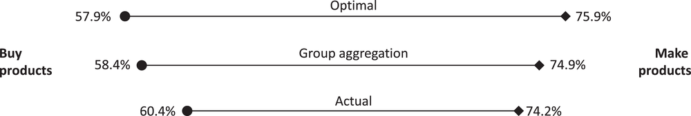
In the optimal solution, the manufacturer considers demand uncertainties, unit revenues, and unit costs when making service‐level decisions (Theorem 2). Because the factors differ across products, the optimal service levels differ across products. The left graph in Figure 2 shows the average optimal service levels for all products and compares them with the average actual service levels.

FIGURE 2

Average actual versus optimal service levels in the product portfolio

We observe heterogeneity in the actual average service levels, which indicates that the manufacturer differentiates service levels by product. However, the correlation between the average actual and optimal service levels of 0.281 is significantly below 1 (

p < 0.001

) and only weakly significantly different from 0 (Kendall's tau,

p = 0.061

), which indicates that the manufacturer uses a different approach than the one suggested by the analytical model.

Determining the optimal service levels for 23 individual products is complex, and a simpler approach is to differentiate service levels by grouping products into categories. In discussions with the retailer and manufacturer, products were often categorized into Make and Buy products. Although customers cannot distinguish between the two categories, the retailer and manufacturer are aware of the differences in profitability. This is also reflected by Make products having a higher average critical ratio than Buy products (

C R_{M a k e}

= 38.7%,

C R_{B u y}

= 28.6%). Therefore, it is optimal to choose higher service levels for Make products than for Buy products. To analyze whether such a differentiation is used by the manufacturer, we analyze the service levels in each product category.

The middle and right graphs in Figure 2 show the results. We observe a higher average actual service level for Make than for Buy products. Within each product category, the average actual and optimal service levels are not significantly correlated (Kendall's tau,

p > 0.528

). This indicates that the manufacturer differentiates service levels by product category but does not differentiate service levels within product categories as suggested by the analytical model. However, we observe variations in the average actual service levels across products and next analyze potential drivers behind the variations.

Summarizing the analyses of this section, we find evidence that the manufacturer has made effective but inefficient decisions. The manufacturer is essentially achieving the target service level, but the differentiation of the products is not optimal and rather focused on the distinction between Make and Buy products. Therefore, we will apply the grouping model (Section 3.2.1) to this special case of two groups. We will extend the analysis to other groupings in Section 4.5. In the next section, we will discuss the data in more detail and test our behavioral models for the manufacturer's decisions.

Evaluation of behavioral models

Before estimating the behavioral parameters and comparing the behavioral models, we will discuss some specifications and general insights regarding the two subtasks forecasting and inventory management.

Behavioral forecasting

The manufacturer faces autocorrelated demand and has not observed sales of the previous day when deciding the order quantity for the current day. For instance, when determining the order quantity for Friday, the manufacturer has not yet seen Thursday's demand and must rely on information from Wednesday and earlier days and weeks.

Figure 3 shows the autocorrelation of demand. It suggests that the manufacturer's best choice is to use demand information from the same weekday in previous weeks because the autocorrelation of the demand is the highest for a time lag of six days. Note that stores are closed on Sundays so that six days correspond to one week. The figure also shows that weekly autocorrelation is higher than daily autocorrelation (dotted bar), which has commonly been observed in grocery retailing environments (van Donselaar et al., 2006, 2010). Therefore, we will use a time lag of one week in the forecasting model. For notational convenience, we denote the current day by

t

and the same weekday of the following week by

t + 1

. We estimated the optimal smoothing factor

η

for our data set by minimizing the mean squared forecast error. The optimal smoothing factor is

η^{*} = 0.25

. Given the optimal

η^{*}

, our setting corresponds to a “low‐adjustment” case in Kremer et al. (2011) and we expect an overadjustment (

b > 1

). We will estimate the parameter below.

FIGURE 3

Autocorrelation coefficients of demand for various time lags

Behavioral inventory management—Group aggregation

We compare the actual service levels with the service levels of the analytical solution. For our grouping model (Section 3.2.1), we assume a Make and Buy grouping as discussed in Section 4.3. We find that service‐level differentiation between products is not as strong as predicted by the analytical model. Figure 4 illustrates the service levels of the two product groups for the optimal solution, the Make‐Buy group aggregation model, and the actual orders. We observe that the group aggregation model results in service levels that are closer to the actual service levels than those of the optimal solution. We note that this effect does not need any estimated parameter, but is the result of optimizing target service levels only for the two product groups.

FIGURE 4

Average service levels for Make and Buy products for optimal differentiation, group optimization, and average actual service level

However, Figure 4 also shows that there remains a gap between the service levels of the group aggregation model and the actual average service levels. This difference might be explained by anchoring (on target service level) and inventory error minimization and we will analyze the behavioral models in detail next. We note that anchoring on mean demand cannot explain the ordering behavior that we observe. If the manufacturer anchored order quantities on mean demand and insufficiently adjusted them toward the target service level, we would observe service levels between 50% and 70%. However, the manufacturer essentially achieves the target service level of 70%, which indicates that the manufacturer does not use mean demand as an anchor. This supports our modeling in Section 3.2.2.

Model estimation and evaluation

Before estimating the different behavioral models from Table 1, we first analyze how well the optimal decision model fits the empirical data. The rational model will serve as a reference point.

Column Optimal of Table 3 reports the fit of the normative solution, that is, the solution with a behavioral forecasting factor of

b = 1

and with optimal product‐specific service levels. To take into account that we fitted coefficients in Models 1–6 and did not fit coefficients for the optimal model, we analyze the Bayesian information criteria (BICs) of the models to compare model fits. For convenience of interpretation, we report the difference in the BICs (

Δ

BIC) of the models relative to the smallest BIC of all models analyzed, that is, Model 6.

TABLE 3

Maximum‐likelihood estimation of behavioral model parameters and quality of fits

	Optimal	Model 1	Model 2	Model 3	Model 4	Model 5	Model 6
Behavioral forecasting factor ( $b$ )		1.750***	1.790***	1.810***	1.790***	1.750***	1.790***
		(0.045)	(0.038)	(0.031)	(0.038)	(0.031)	(0.039)
Group service levels^a
‐ Make products ( $α_{M}$ )			0.584		0.591		0.590
‐ Buy products ( $α_{B}$ )			0.749		0.746		0.747
Anchoring factor ( $a$ )				0.493***	0.057***
				(0.004)	(0.007)
Inventory error
‐ Psychological overage cost ( $δ_{o}$ )						4.219***	0.003
						(0.127)	(0.010)
‐ Psychological underage cost ( $δ_{u}$ )						3.045***	0.223***
						(0.135)	(0.043)
Log‐likelihood	−541,160	−537,851	−530,431	−531,356	−530,401	−531,036	−530,385
BIC	1,082,331	1,075,714	1,060,874	1,062,737	1,060,826	1,062,110	1,060,807
$Δ$ BIC^b	21,524	14,907	67	1,930	19	1,303	0
MCS^c	$<$ 0.0001	$<$ 0.0001	0.008	$<$ 0.0001	0.019	$<$ 0.0001	x

Abbreviations: BIC, Bayesian information criteria; MCS, model confidence set.

Values are the results of an optimization, not of a parameter estimation. Therefore, no significance can be reported.

Δ

BIC is the difference between the BIC of the model and the lowest BIC of all models.

Model with “x” is included in the MCS, for other models the p‐value for exclusion is reported.

***

< 0

.01,

^{* *}

<

0.05, and

^{*}

<

0.10; standard errors are in parentheses.

To estimate the behavioral forecasting factor

b

, we used the behavioral forecasting model in the analytical optimization models (3) and (4) and conducted a maximum‐likelihood estimation of the factor. For given values of

b

, we determined the order quantities for each store, product, and day and their likelihoods. We chose the parameter value of

b

that resulted in the highest likelihood. To obtain robust estimates for

b

and its standard error, we performed a bootstrap with 100 replications (Boone et al., 2008). Note that we tested the convergence of our estimates over the number of replications (Chernick, 2011) and find that the estimates are already robust for smaller numbers of replications.

Column Model 1 of Table 3 shows the results of the parameter estimation and the value of the likelihood. The behavioral forecasting factor with the highest likelihood is

b = 1.75

and is significantly different from 1 (

p < 0.001

). Thus, we find an indication for overreaction to recent demand observations. To understand the impact of behavioral forecasting, we analyze the forecasts and the resulting root mean squared error (RMSE). We find that the mean of the behavioral forecasts is similar but with slightly higher RMSE. On average, the mean is 0.34% smaller under the behavioral forecast compared to the optimal forecasting, while RMSE increases by 3.48% under the behavioral forecast compared to optimal forecasting. We conclude that behavioral forecasting decreases the forecasting performance. Detailed analyses on the monetary impact of this factor will be shown in Section 4.6.

Model 1 has a smaller BIC than the optimal model and we conclude that including behavioral forecasting explains the manufacturer's ordering behavior better than the optimal model without. The magnitude of the differences in the BICs is large and we will include behavioral forecasting in all other models. We cannot use the chi‐square test to compare our models because not all of them are nested. To compare all models analytically, we will use the model confidence set (MCS) at the end of this section (Hansen et al., 2011).

Column Model 2 of Table 3 shows the results of the group model optimization. The optimal group service levels are the results of the optimization. The behavioral forecasting factor was determined by maximum‐likelihood estimation using the same approach that we used for estimating

b

in Model 1. The likelihoods and BICs indicate that the group aggregation model has a significantly better fit than Model 1 and than the optimal model.

In Models 3 and 4, the anchoring factor

a

is significantly different from 0. To analyze whether anchoring provides a better explanation of the manufacturer's ordering behavior than does group aggregation, we compare the BICs of Models 2 and 3. The BIC of Model 3 is 1,863 above that of Model 2 and we conclude that the individual anchoring model is performing worse than the group aggregation model.

To analyze whether group anchoring, which uses anchoring in addition to group aggregation, improves the fit of the model, we compare the BICs of Models 2 and 4. The BIC of Model 4 is 48 below that of Model 2, indicating that anchoring in addition to group aggregation explains actual orders better than without anchoring.

Inventory errors: To estimate the psychological underage and overage cost, we use an approach similar to the one for the behavioral forecasting parameter

b

, and compute the order quantities for given psychological overage and underage costs. In Model 5, the psychological costs are positive and significantly different from 0 (

p < 0.01

) and the fit of Model 5 (BIC = 1,062,110) is significantly better than that of Model 1 (BIC = 1,075,714). In line with Ho et al. (2010), the psychological overage costs

δ_{o}

are greater than psychological underage costs

δ_{u}

Including group aggregation improves the fit further, which gives Model 6 the best fit of all the models that we analyzed. Incorporating the group aggregation bias, the value of the psychological costs decreases significantly and

δ_{o}

is no longer significant. Although the fit of Model 6 (BIC =1,060,807) is much better than that of Model 5 (BIC = 1,062,110), the difference between Models 6 and 2 (group aggregation only, BIC = 1,060,874) is fairly small.

We also analyzed whether Make and Buy products have different forecasting biases and estimated group‐specific

b

. We estimate

b_{M a k e} = 1.83

and

b_{B u y} = 1.15

for Model 1 (estimates are similar for Model 2). We find that both groups show significant forecasting biases with a stronger overreaction for Make products. We analyzed the potential impact of group‐specific forecasting factors on the estimates in Models 3–6 but found only small differences (e.g., for Model 5,

δ_{o} = 3.92

and

δ_{u} = 3.11

for using

b_{M a k e} = 1.83

and

b_{B u y} = 1.15

). Therefore, the findings and conclusions hold for both approaches.

In total, we analyzed six behavioral models, and the results indicate that including behavioral forecasting and group aggregation is important for understanding the manufacturer's ordering behavior. The results also indicate that including anchoring or inventory error minimization in the models further improves the fit. These two factors result in actual service levels being pulled‐to‐target (i.e., Buy products being pulled upward, and Make products being pulled downward). However, compared with the model including behavioral forecasting and group aggregation (Model 2), the additional improvements obtained by including anchoring (Model 4) or inventory error minimization (Model 6) are comparable, and it is not obvious which model provides the best fit.

Selecting the model based on the BIC does not reveal the uncertainty of this selection (Hansen et al., 2011). To determine whether the differences in the model fits are significant, we use the MCS introduced by Hansen et al. (2011). The MCS conducts a sequence of hypothesis tests based on bootstrap samples and eliminates the models that are significantly outperformed at a given

p

‐value. Like Eichler et al. (2014), we use

p = 0.05

and 1,000 bootstrap samples.

The results of the MCS are also shown in Table 3. For our data, the MCS consists of a single model, Model 6. This model performs weakly significantly better than Model 4 (

p = 0.019

), and highly significantly better than all other models (

p < 0.01

). We conclude that a model with behavioral forecasting, group aggregation, and inventory error minimization explains the manufacturer's ordering behavior best, but the latter has only a small effect compared to the first two decision biases.

Other grouping heuristics

In Section 3.2.1, we argued that the categorization into Make and Buy products is a natural differentiation of products for the manufacturer. Additionally, the analysis in the previous section indicated that this grouping heuristic fits actual decisions well. However, there are other potential groupings, and we analyze some of them that seem reasonable to follow.

Clustering the products by product type could be an appropriate categorization. Setting target service levels for breads (type 1), rolls (type 2), and pastries (type 3) would provide an alternative intuitive clustering. Although this requires three target service levels, the decision process is still significantly easier than determining 23 targets.

Management literature often uses ABC analysis to differentiate inventory policies for different products. Table 2 also shows the ABC classification for the 23 products in our assortment. Using this categorization, a grouping heuristic could optimize the target service levels for these categories.

A very basic alternative clustering would be to use only one group. This means that all products receive the same target service level. We refer to this as “naive” approach because it uses the target service level (of 70%) for each of the products.

We conducted comparable analyzes as in Section 4.4.3 for the three alternative grouping models. We used the classifications to determine the optimal target service level and the resulting order quantities for each day in our data set. We then conducted a maximum‐likelihood estimation for these predictions on our data set. Table 4 shows the change in BIC when using the alternative groupings compared to the Make–Buy classification. We find that the alternative groupings explain the manufacturer's decisions not as well as the Make–Buy grouping. Figure B.1 also compares the actual average product service levels with the predicted service levels achieved by the different grouping heuristics. The graphs show that predicted product service levels are closer to actual service levels for the Make–Buy clustering than for the other groupings analyzed.

TABLE 4

Comparing the fit of alternative grouping models

	Make–Buy	ABC	Product type	Naive
$Δ$ BIC	0	13,621	16,765	14,291

FIGURE 5

Determining the profit impact of the detected decision biases

FIGURE 6

How to improve performance: profit impact of different grouping heuristics compared with optimal differentiation (normalized to 100%)

Managerial implications—Impact on profit and potential recommendations

Our analyses indicate that the manufacturer's ordering decisions are affected by three biases: behavioral forecasting, group aggregation, and inventory error minimization. These biases are significant and explain actual ordering decisions better than the other biases or combinations of biases that we analyzed. However, from a managerial perspective, not only the significance of effects but also their monetary impact is important. Therefore, we evaluate the impact of the three different behavioral factors on the manufacturer's profitability.

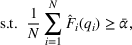
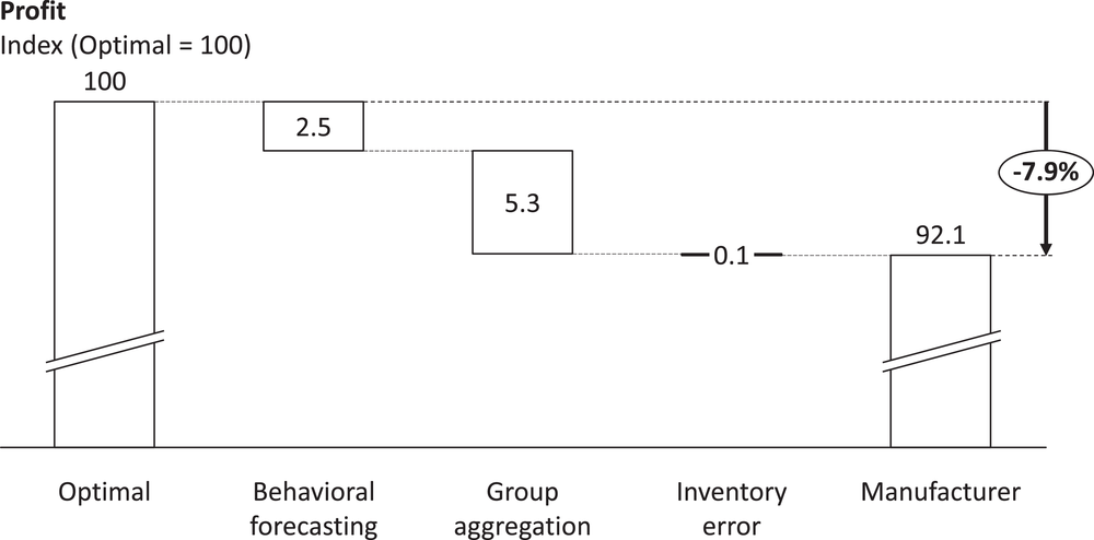
We simulate the use of different decision models and calculate the resulting profit for our data set. We forecast demand for each product in each store, determine the resulting order quantity, and calculate the resulting profit based on actual demand. To calculate profits for the different models for our data set, we must estimate demand (given the unobservable lost sales) based on sales data. We estimate demand based on the approach of Lau and Lau (1996), which uses stockout times and hourly demand information from previous periods to estimate unobservable lost sales. Note that this approach is different from the one used in the analytical model because stockout times are not available to the manufacturer and therefore cannot be used in demand forecasting. However, an approach considering stockout timing provides more accurate demand estimates (Jain et al., 2015) and enables an accurate profit comparison between different analytical models and the manufacturer's decisions. Figure 5 shows the reduction of profit allocated to the different behavioral aspects. As a benchmark, we indexed the profit of the optimal solution at 100. This means with the data available by the manufacturer (historical number of units sold) and using nonbiased forecasting and optimal product differentiation the manufacturer would achieve a profit of 100.

To estimate the impact of the different behavioral factors, we calculate the profits of partial models, including the different factors sequentially. We calculate the predicted order quantities for using the behavioral models (with the estimated parameters in Table 3) and simulate the performance for our data set. Applying behavioral forecasting, but keeping the optimal differentiation, results in a profit decrease of 2.5% compared to the optimal model. When further including group aggregation on these biased forecasts, profits decrease by another 5.3%. The effect of inventory error minimization is small compared to the other two effects (only 0.1% profit loss). The results suggest that substantial profit gains can be achieved by reducing decision biases.

The total profit that the manufacturer actually achieved is 92.2. As a robustness check, and as a fair comparison with our partial models, we calculated the profits using order quantities resulting from the model containing all three decision biases (Model 6 in Table 3). The resulting average profits are 92.1, which is close to the actual profits. The results indicate a profit loss of 7.9% that can be attributed to the decision biases.

Behavioral forecasting or including psychological inventory error costs does not help to reduce complexity. For instance, behavioral forecasting distorts demand forecasts without significantly reducing effort. In such cases, debiasing strategies might be applicable to improve performance. Decomposing forecasting and inventory decisions (Lee & Siemsen, 2017) or using multiple independent forecasters (Kremer et al., 2011) might reduce the forecasting bias and improve overall performance.

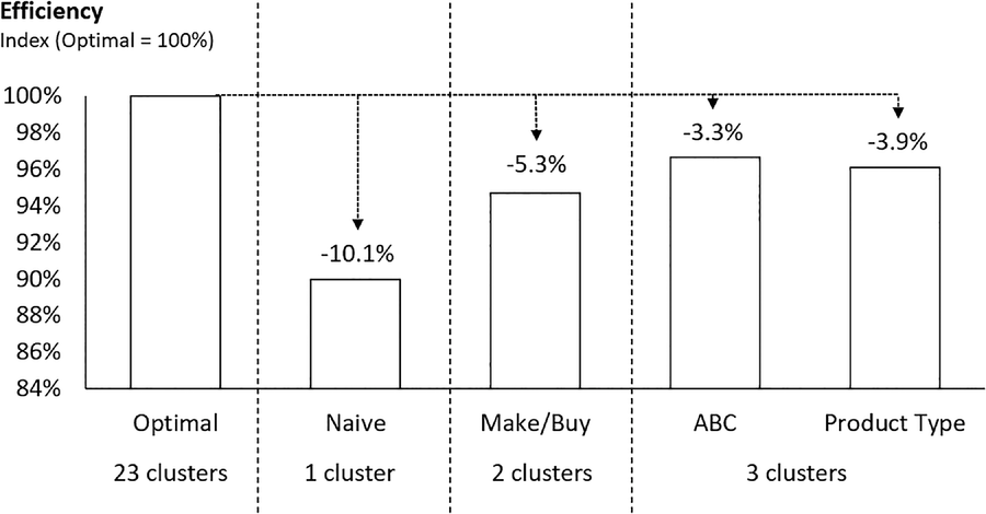
However, we have seen that group aggregation has a major profit impact. In general, using grouping heuristics might simplify the decision tasks of the manufacturer but results in efficiency losses. To analyze the impact of such heuristics on profits, we simulate the performance of different grouping heuristics. Figure 6 shows the profit losses for four grouping models compared to optimal differentiation. Using a naive no‐differentiation approach (i.e., targeting 70% for all products) reduces profits by 10.1%. Note that we used nonbiased forecasting for these analyses to isolate the impact of the grouping heuristics. Therefore, adding this simple differentiation (Make vs. Buy) already leads to a substantial improvement in profits over naive optimization with rather limited additional effort (only two different target service levels). Make–Buy grouping results in a profit loss of 5.3%. Increasing the number of clusters, for example, to three, decreases the efficiency loss further. But we see that the marginal improvement decreases. Using the ABC analysis based clustering and the clustering by product type (bread, rolls, pastries) that were introduced in Section 4.5, results in profits losses of 3.3% and 3.9%. This means that the manufacturer could increase his profits by adding a third group. However, marginal gains of adding another group decrease and using the Make–Buy grouping captures the majority of the potential differentiation gains. This implies that given the increasing complexity and the decreasing marginal benefits of adding groups, grouping heuristics might be considered ecologically rational (Gigerenzer & Todd, 2012), which is related to Simon's (1986) idea of satisficing. Adding more groups would increase profitability of the manufacturer, but (perceived) additional required effort might prevent the manufacturer from doing so. Additionally, Chen and Li (2018) compare the performance of human decision makers when making a single decision versus multiple simultaneous decisions. They find that performance decreases when making multiple decisions. This indicates that increasing the number of groups from two to three might not result in the additional profit indicated in Figure 6 due to the increased complexity of the decision task.

DISCUSSION

The ordering behavior of newsvendor decisions in laboratory environments has been analyzed extensively over the past two decades (Donohue et al., 2020). The experiments were usually conducted with students who entered orders in a computer over a short period of time to earn a moderate amount of money. In practice, experienced managers place orders for real products on a daily basis and their performance affects their incomes and their careers. Previous experiments therefore left unclear whether the decision biases observed in the laboratory were also present in practice.

In this paper, we address this issue by analyzing the ordering behavior of an actual manufacturer. The results of our analyses indicate that the decision biases that have been observed in laboratory experiments are also present at the manufacturer (e.g., behavioral forecasting and ex‐post inventory error minimization). We identified an additional bias: group aggregation. Although the manufacturer is prone to these biases, his decisions resulted in effective solutions with service levels that were close to the target service level of 70%. This result is of some interest in its own right. One of the most robust findings of the behavioral operations management literature is that decision makers choose order quantities that are pulled toward the expected demand (e.g., Bolton & Katok, 2008; Bostian et al., 2008; Schweitzer & Cachon, 2000). Translated to the manufacturer's situation, it suggests that the service levels are below the target service level and are pulled toward 50%. This, however, is not what we observed.

The main reason for this is the specific setting that the manufacturer faces. The manufacturer operates under a service level contract, whereas most laboratory experiments (showing the pull‐to‐center bias) use profit‐based contracts such as wholesale price or buyback contracts. As Bolton et al. (2016) show in lab experiments, decision makers achieve target service levels more effectively and more efficiently under a service‐level contract than using a wholesale price contract. Potential reasons are that the service‐level contract provides an anchor that the wholesale price contract does not provide and that the expected profit curve is steeper. Related to this, Lee and Siemsen (2017) find a strong performance increase when providing the optimal target service level in profit‐based environments such as the wholesale price contract setting. Although our setting does not include service‐level penalties (that are used in Bolton et al., 2016), the manufacturer still has an explicit service‐level constraint of 70% that he is not allowed to fall below. This results in overall average service levels that are not pulled‐to‐center, but rather pulled‐to‐target, which means that differentiation between products is not strong enough.

Looking at the efficiency loss of the decision maker, we find that the manufacturer incurs a profit loss of 5.3% compared to our analytical model. One might argue that the performance is actually not too bad compared to subjects in newsvendor lab experiments. However, we want to highlight three important aspects here. First, previous lab studies using single product newsvendor settings report a range of efficiencies between 80% (Bolton & Katok, 2008) and 89% (Bolton et al., 2012, for trained subjects) depending on experience and prior knowledge. We acknowledge that our empirical setting is more complex, but the decision maker is also much more experienced than subjects in the lab. Therefore, seeing higher efficiencies is not very surprising. Using a single‐product service‐level contract, Bolton et al. (2016) report efficiencies between 89% and 97.2%. This shows that service‐level contracts lead to higher performance also in the lab environment.

The second important aspect that needs to be considered when comparing our empirical results with previous lab data is that we have provided a model for optimizing order quantities for the multiproduct problem that the manufacturer faces. Like all analytical models, our model relies on a number of assumptions. We expect that more comprehensive models would improve profits further, but they are also much more complex. This would increase the efficiency loss of the decision maker compared to the optimal model. Lab studies compare actual decision making against the normative benchmark.

Third, the manufacturer is subject to self‐selection and market selection, whereas subjects in laboratory studies are typically selected on a first‐come‐first‐serve basis out of a pool of students looking for some short‐term financial benefit. Thus, the consequences of ordering suboptimally are quite different for students and for the manufacturer. If the manufacturer does not achieve the target service level, he loses business with the retailer and is replaced by another manufacturer. Therefore, it is not surprising that we observe a manufacturer who is achieving the target service level with a rather moderate efficiency loss. If efficiency had been far below optimum, other companies would probably have taken over the business already.

Highlighting the differences between our empirical setting, existing lab studies, and the impact of different grouping heuristics, we acknowledge that it might be insightful to analyze decision making in this context in more detail in future lab studies. Using multiproduct cases with differentiation between products has not been studied extensively. Such lab experiments could complement our findings, and improve the understanding of behavioral decision making in operations management even further. This might also allow to analyze behavioral factors such as cognitive limitations, sacrificing, or time pressure in more detail.

Footnotes

PROOFS

ADDITIONAL GRAPHS—PREDICTIVE FIT OF PRODUCT SERVICE LEVEL

ACKNOWLEDGMENTS

We thank the department editor Elena Katok, the senior editor, and two anonymous referees for their constructive comments to improve the paper. We also thank the German Research Foundation for financial support through the research unit “Design & Behavior” (FOR 1371) and Germany's Excellence Strategy—EXC 2126/1.

ORCID

Anna‐Lena Sachs

Michael Becker‐Peth

Stefan Minner

Ulrich W. Thonemann

References

Becker‐Peth

Thonemann

(2018). Behavioral inventory decisions: The newsvendor and other inventory settings. In Donohue

Katok

Leider

(Eds.), The handbook of behavioral operations (pp. 393–432). John Wiley & Sons.

Bell

(1981). Adaptive sales forecasting with many stockouts. Journal of the Operational Research Society, 32(10), 865–873.

Benzion

Cohen

Peled

Shavit

(2008). Decision‐making and the newsvendor problem: An experimental study. Journal of the Operational Research Society, 59(9), 1281–1287.

Bolton

Katok

(2008). Learning by doing in the newsvendor problem: A laboratory investigation of the role of experience and feedback. Manufacturing & Service Operations Management, 10(3), 519–538.

Bolton

Ockenfels

Thonemann

(2012). Manager and students as newsvendors. Management Science, 54(12), 2225–2233.

Bolton

Stangl

Thonemann

U. W.

(2016). Decision making under service level contracts—An experimental analysis . https://ssrn.com/abstract=2838645

Boone

Ganeshan

Hicks

R. L.

(2008). Learning and knowledge depreciation in professional services. Management Science, 54(7), 1231–1236.

Bostian

Holt

Smith

(2008). Newsvendor pull‐to‐center effect: Adaptive learning in a laboratory experiment. Manufacturing & Service Operations Management, 10(4), 590–608.

Chatfield

(2001). Time‐series forecasting. Chapman & Hall.

10.

Chen

K.‐Y.

(2018). The behavioral traps in making multiple, simultaneous, newsvendor decisions . https://ssrn.com/abstract=2817126

11.

Chernick

M. R.

(2011). Bootstrap methods: A guide for practitioners and researchers (Vol. 619). John Wiley & Sons.

12.

Choi

T.‐M.

(2012). Handbook of newsvendor problems: Models, extensions and applications (Vol. 176). Springer.

13.

Donohue

Özer

Ö.

Zheng

(2020). Behavioral operations: Past, present, and future. Manufacturing & Service Operations Management, 22(1), 191–202.

14.

Edgeworth

F. Y.

(1888). The mathematical theory of banking. Journal of the Royal Statistical Society, 51(1), 113–127.

15.

Eichler

Grothe

Manner

Tuerk

(2014). Models for short‐term forecasting of spike occurrences in Australian electricity markets: A comparative study. Journal of Energy Markets, 7(1), 245–266.

16.

Feiler

D. C.

Tong

J. D.

Larrick

R. P.

(2013). Biased judgment in censored environments. Management Science, 59(3), 573–591.

17.

Gigerenzer

Todd

P. M.

(2012). Ecological rationality: The normative study of heuristics. In Ecological rationality: Intelligence in the world (pp. 487–497). Oxford University Press.

18.

Goodwin

Moritz

Siemsen

(2018). Forecast decisions. In Donohue

Katok

Leider

(Eds.), The handbook of behavioral operations (pp. 433–458). John Wiley & Sons.

19.

Hansen

Lunde

Nason

(2011). The model confidence set. Econometrica, 79(2), 453–497.

20.

Lim

Cui

(2010). Reference dependence in multilocation newsvendor models: A structural analysis. Management Science, 56(11), 1891–1910.

21.

Jain

Rudi

Wang

(2015). Demand estimation and ordering under censoring: Stock‐out timing is (almost) all you need. Operations Research, 63(1), 134–150.

22.

Katok

(2009). Contracting in supply chains: A laboratory investigation. Management Science, 55(12), 1953–1968.

23.

Kremer

Minner

Van Wassenhove

(2010). Do random errors explain newsvendor behavior? Manufacturing & Service Operations Management, 12(4), 673–681.

24.

Kremer

Minner

Van Wassenhove

(2014). On the preference to avoid ex‐post inventory errors. Production and Operations Management, 23(5), 773–787.

25.

Kremer

Moritz

Siemsen

(2011). Demand forecasting behavior: System neglect and change detection. Management Science, 57(10), 1827–1843.

26.

Lau

Bearden

J. N.

(2013). Newsvendor demand chasing revisited. Management Science, 59(5), 1245–1249.

27.

Lau

H.‐S.

Lau

A. H.‐L.

(1996). Estimating the demand distributions of single‐period items having frequent stockouts. European Journal of Operational Research, 92(2), 254–265.

28.

Lee

Y. S.

Seo

Y. W.

Siemsen

(2018). Running behavioral operations experiments using Amazon's Mechanical Turk. Production and Operations Management, 27(5), 973–989.

29.

Lee

Y. S.

Siemsen

(2017). Task decomposition and newsvendor decision making. Management Science, 63(10), 3226–3245.

30.

Lurie

N. H.

Swaminathan

(2009). Is timely information always better? The effect of feedback frequency on decision making. Organizational Behavior and Human Decision Processes, 108(2), 315–329.

31.

Lysons

Farrington

(2006). Purchasing and supply chain management. Pearson Education.

32.

Moritz

Hill

Donohue

(2013). Individual differences in the newsvendor problem: Behavior and cognitive reflection. Journal of Operations Management, 31(1), 72–85.

33.

Ockenfels

Selten

(2015). Impulse balance and multiple‐period feedback in the newsvendor game. Production and Operations Management, 24(12), 1901–1906.

34.

Schweitzer

Cachon

(2000). Decision bias in the newsvendor problem with a known demand distribution: Experimental evidence. Management Science, 46(3), 404–420.

35.

Simon

(1986). Rationality in psychology and economics. Journal of Business, 59(4), 209–224.

36.

Teunter

R. H.

Babai

M. Z.

Syntetos

A. A.

(2010). ABC classification: Service levels and inventory costs. Production and Operations Management, 19(3), 343–352.

37.

Tong

Feiler

(2017). A behavioral model of forecasting: Naive statistics on mental samples. Management Science, 63(11), 3609–3627.

38.

Tversky

Kahneman

(1974). Judgment under uncertainty: Heuristics and biases. Science, 185(4157), 1124–1131.

39.

vanDonselaar

Gaur

vanWoensel

Broekmeulen

Fransoo

(2010). Ordering behavior in retail stores and implications for automated replenishment. Management Science, 56(5), 766–784.

40.

vanDonselaar

vanWoensel

Broekmeulen

Fransoo

(2006). Inventory control of perishables in supermarkets. International Journal of Production Economics, 104(2), 462–472.

41.

Wecker

(1978). Predicting demand from sales data in the presence of stockouts. Management Science, 24(10), 1043–1054.

Empirical newsvendor biases: Are target service levels achieved effectively and efficiently?

Abstract

Keywords

INTRODUCTION

ANALYTICAL MODEL

Demand forecasting

Newsvendor system approach

BEHAVIORAL MODELS

Behavioral demand forecasting

Behavioral inventory optimization

Group aggregation

Anchoring

Inventory error minimization

EMPIRICAL DECISION ANALYSIS

Setting and data

Service levels by store

Service‐level differentiation by product

Evaluation of behavioral models

Behavioral forecasting

Behavioral inventory management—Group aggregation

Model estimation and evaluation

Other grouping heuristics

Managerial implications—Impact on profit and potential recommendations

DISCUSSION

Footnotes

PROOFS

ADDITIONAL GRAPHS—PREDICTIVE FIT OF PRODUCT SERVICE LEVEL

ACKNOWLEDGMENTS

ORCID

References