
Abstract
In this paper, we reflect on the supply chain issues and operational challenges that we experienced through the various stages of the Covid‐19 pandemic. We identify some phenomena that were attributable in some way to the pandemic, and apply core principles of operations management, and a simple numerical model, to explain and understand their occurrence. We highlight some key lessons and discuss implications for supply chain design and planning, to prepare for the next global disruption.
Keywords
INTRODUCTION
A supply chain connects supply to demand. Over the course of the Covid‐19 pandemic, we witnessed countless events that disrupted or distorted supply chains in some way for some duration. Some of the events mainly affected the demand served by a supply chain, while others mainly affected the supply side. We will first discuss demand events, and use a simple model to examine the challenges of managing through a demand event. We will then look at supply events and do the same. We will conclude with some lessons and implications for operations management
We limit the scope primarily to abnormal impacts on our common supply chains that were attributable in some way to the pandemic. We exclude other disruptions that we recently experienced, for example, due to blockage in the Suez Canal, or due to extreme weather events. Our main sources for our observations are from the media coverage of supply chain events. We do not try to formally or carefully cite these sources; rather, we provide in the Appendix a list of newspaper articles that are representative of what we learned and experienced over the course of the pandemic.
Our intent is to reflect on recent supply chain phenomena from the pandemic and to extract lessons that, for instance, could be shared in the future with our students. We do not develop any new theory or models to do so. Rather, we rely on established ideas and mental models from operations management to explain what happened to our supply chains and why. We then use these findings to identify guidelines and research opportunities for the planning and management of supply chains in the future.
Before reviewing the supply chain disruptions from the pandemic, we use the 30th anniversary of
Kleindorfer and Saad (2005) establish the specify–assess–mitigate (SAM) framework precisely for disruptions outside a company's normal supply–demand process. It is rigorous and comprehensive in its scope, with demonstrated applicability to the chemical industry. Sodhi et al. (2011) conduct a broad field research study including practitioners and academics that identifies three gaps in supply chain management research. The pandemic highlights that those gaps are still present today. Namely, supply chain disruption does not have a consistent definition, the recovery process from disruptions is poorly studied, and an empirical study of disruptions is lacking.
While not focused on the supply chain dynamics underlying a disruption, Hendricks and Singhal (2005) quantify the significant impact disruption announcements have on a firm's stock price. Their work documents disruptions as transient events that are not quickly recovered from.
In the category of “what is old is new,” Clark (1996) and Hayes and Pisano (1996) demonstrate that the “advanced manufacturing system (AMS),” comprised of now‐standard improvement methodologies including just‐in‐time (JIT) and statistical process control (SPC), is insufficient to improve the company's cost–variety performance frontier. Of particular relevance to the pandemic is the recognition that strategic decisions consciously make structural choices between alternatives in order to define and shape a company's performance frontier. The corollary to this recognition is that a company that is not making strategic decisions, and only relying on AMS, leaves itself vulnerable to disruption.
In the next section, we describe some of the demand events that disrupted supply chains during the pandemic. We then pose a stylized model of a retailer and a supplier, as a mechanism for exploring the supply chain dynamics induced by a demand event. We illustrate these dynamics with deterministic simulations. We then use the stylized model to illustrate the supply chain dynamics that result from a supply disruption. We provide next some observations and lessons from these numerical exercises; we conclude with a discussion of some implications for operations management, particularly in terms of future research opportunities.
SUPPLY CHAIN PHENOMENA: DEMAND EVENTS
At the start of the pandemic, with the lockdowns and restrictions, our world was turned upside down. The GDP for the United States dropped dramatically in the first half of 2020, with most of that happening in the second quarter; real and current‐dollar GDP both declined by more than 30% in the second quarter of 2020. 1 With stimulus from federal payouts, the economy recovered very quickly in the second half of 2020, with the recovery continuing strongly through 2021. Over these 2 years, there was a full range of demand impacts affecting nearly all products and their supply chains. We cite next some examples, with a simple categorization.
One‐time surge
At the onset of the pandemic, with the lockdowns, demand for home supplies like toilet paper spiked, as consumers hoarded essential items; presumably this was driven by fear that supplies would become unavailable. There was also a spike in consumer demand (and hoarding) of home supplies needed to respond to the pandemic, for example, masks and hand cleansers. There was a similar spike for medical equipment, like ventilators, that would be needed for Covid patients. More recently, we saw a spike in demand for test kits as the pandemic became endemic.
Sustained increase in demand
With families at home, demand increased in several categories such as home furnishings, home improvement supplies, equipment and supplies needed for remote work and at‐home schooling, and exercise equipment. There was also a spike in clinical demand (and hoarding) of medical supplies needed to respond to the pandemic, for example, masks, personal protective equipment (PPEs), and disinfectants; after the initial spike, there has been sustained demand that has followed the waves of the pandemic.
Drop in demand
At the onset of the pandemic, with the lockdowns and overall uncertainty about the course of the pandemic, demand for automobiles, and other durables and luxury items, dropped dramatically. For a month or two, the economy contracted. At the same time, with families at home, demand for travel‐related products and services dropped dramatically.
Change in channel
There were many instances for which there was a change in the supply channel through which demand was served. This resulted at times in a dramatic increase in demand for one channel, while demand for the alternate channel dropped. The most prominent example has been the increase in online retailing throughout the pandemic. Many brick and mortar stores were initially closed, some never reopened, and as others did open, some customers were reluctant to shop in person; furthermore, online retailing benefited from its virtuous cycle—as more customers experienced online shopping, they become more dependent on it.
Similarly, with restaurants and cafeterias closed or restricted, the demand for institutional food (i.e., food served in restaurants and cafeterias) dropped, while food destined for home consumption increased (i.e., food sold in supermarkets). The aggregate demand for some food categories was also affected; for instance, the demand for fresh fish dropped as the preponderance of fresh fish is consumed in restaurants and cafeterias. There were similar demand impacts for office supplies, as offices closed and people worked remotely from home.
It is noteworthy that each of these demand phenomena could not have been predicted for any particular product at the start of 2020 prior to the pandemic. Even in the early weeks and months of the pandemic, one would have been hard pressed to have foreseen what was to come. Whereas these phenomena were each “obvious” in hind sight, at the time, with the uncertainty about the virus and its course, as well as with the ever‐evolving response strategies, one would have needed a crystal ball to see many of these changes. Similarly, the persistence or trajectory of any demand change was also highly uncertain. As just one example, as we write this paper at the start of 2022, we have a spike in demand for rapid test kits; it is very hard to know whether this demand increase will persist for the remainder of 2022 or go quickly away. 2
SIMPLE MODEL ON SUPPLY CHAIN DYNAMICS: DEMAND EVENTS
These demand events created unprecedented challenges for many supply chains. To appreciate these challenges, we have developed a simple numerical model of a simple, stylized supply chain. The intent is to provide some explanation for why our supply chains have struggled in response to these demand events, and from this, to extract some lessons that might guide future supply chains in their preparation, planning, and response.
For our model, we consider a store that sells toilet paper (or exercise bikes, hand cleanser, masks, disinfectant, pet food). Historically, demand is quite stable, at around 100 units per week. The store replenishes weekly from a supplier with reliable lead‐time of 4 weeks.
Suppose, however, in a given week, there is a demand spike to 300. The store has sufficient inventory to handle the spike, but at end the week, it has depleted much of its safety stock.
What should the store do? In particular, what should the store order from the supplier? Should the store share any other information with its supplier?
Based on inventory theory and practice, the store should order at least enough to bring its inventory position to a level to cover the forecast of demand over the lead‐time. In addition, the store might order more to start to rebuild its safety stock. However, in light of the demand spike, what should be the forecast for the demand over the lead‐time? The weekly demand forecast has been 100; should the store adjust this forecast? The lead‐time has been 4 weeks; should the store expect the lead‐time to remain at 4 weeks or not? At a minimum, the store should order at least 300 units to replace what it just supplied. Beyond this, the store might order more, depending on what it assumes or anticipates.
Model assumptions
To explore this dilemma, we develop a simple numerical model. Our intent is to provide some intuition for the complexity of inventory control in this seemingly simple setting, as well as some understanding of what factors and assumptions drive this complexity. We then discuss how this intuition might guide the choice of tactics to achieve better control. More formally, we assume the following process for setting an order in each period: In week The store makes its forecast of the future weekly demand rate, call it The store determines its order‐up‐to point given by The store then orders With this ordering rule, we can express the inventory position as
We note three implicit assumptions in specifying this ordering rule.


First, we assume that the order placed in week 
Second, we assume in each week that the store updates its forecast of demand, but does not attempt to forecast or anticipate any future changes in the lead‐time; rather, we assume the store uses the current lead‐time as shared by the supplier. One might contemplate how a store would make such a forecast, and add this to the model. We expect that this would add additional dynamics to the model, depending on the assumptions. However, it might also obfuscate any lessons from this exercise. So for now, we have chosen just to include a forecast of the demand rate.
Third, we assume that the store does not adjust its safety stock as conditions change; for the purposes of our analysis, this is a conservative (and simplifying) assumption. Safety stock adjustment is a well‐known driver of the bullwhip effect (Lee et al., 1997); hence, if we were to relax this assumption, we expect our results would show even greater dynamics.
We suppose that the supplier has a capacity of
The supplier's queue at the end of week 


We can also assume that the store shares its demand information, forecast, and ordering logic with the supplier. However, this information does not affect the supplier's decisions, provided we assume that neither the store nor the supplier can cancel any placed orders.
As noted earlier, we assume the store has just observed a demand spike. We pose two possible ‘ground truths’ to consider and evaluate. These are: In the following week, demand returns to normal, 100 per week; the spike represents a In the following week, demand drops to 150, and stabilizes for (say) 3 weeks, and then returns to 100. This represents a
We do not explicitly explore here the two other phenomenon,
The store does not know the ground truth. Nevertheless, to plan its orders, the store has to make a guess about the future. We capture this with the forecast model. If the store thinks the spike is just a one‐time aberration or transient event, then this could correspond to using a very small smoothing parameter (closer to zero) in the forecast model. On the other hand, if the store thinks the spike signals a change in demand, then the smoothing parameter might be set much larger (closer to one), so as to make the forecast model more responsive. If the store is not sure what the spike forebodes, then its forecast might be a compromise with a midlevel smoothing parameter.
Exploration of supply chain dynamics
In the following, we examine the response to each of these two ground truths. We start with an inventory of
One‐time surge
Demand spikes to 300 in week
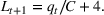
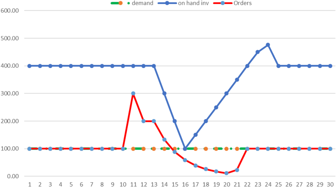
We show in Figure 1 the system behavior with a smoothing parameter α = 0.20 for the forecast model; this corresponds to the store thinking that most of the spike is likely a one‐time aberration. 6
One‐time surge α = 0.20
We see here that even with a reasonable guess that the spike is temporary, the system experiences significant volatility.
The store places a very large order of 460 units in week 10 in response to the spike.
7
This greatly exceeds the capacity at the supplier, and the supplier quotes a longer lead‐time of over 6 weeks. In the following week, week 11, even though the store sees demand return to 100, it still places a substantial order (340) due to the lead‐time increase. This order again exceeds supplier capacity, which results in an even longer lead‐time. As the store continues to see “normal” demand of 100, it brings its forecast back to this level, and starts to reduce its orders. However, the initial large orders, based on a presumption that some of the demand spike might continue, were too much, and the store stops ordering in week 15. The demand spike that raised demand by 200 units from 100 to 300 results in the
The demand spike drops the inventory in week 10 from 400 to 200. There is no further drop in inventory since this is a one‐time demand surge and the demand returns to the normal level thereafter. It then takes the lead‐time of 4 weeks before the supplier starts to fill the large orders and the inventory can start to recover. Starting in week 14, the inventory rebuilds at a rate of 50 units per week, equal to the supplier capacity net of the demand rate (150 – 100). By week 17, the inventory has recovered to its starting level of 400 units, so the
However, we see an extended overshoot as the inventory continues to grow, peaking at 585 in week 21 (4 weeks after the inventory has recovered). This overshoot is due to the overordering immediately after the demand spike. This overordering is due to a “misinterpretation” of the demand spike. The store does not know whether the demand increase from the spike will continue or not, or for how long; in this instance, we assume that the store thinks a small portion (20%) of the demand increase will continue and thus, the store needs to order more. The initial large order increases the lead‐time at the supplier, which induces the store to order even more to cover the longer lead‐time. The supplier's lead‐time of 4 weeks delays the response to the large orders; and then the supplier's capacity of 150 per week gates the rate at which these large orders can be filled. The result is the extended overshoot, which peaks 11 weeks after the spike, with an
The system reverts to stability after the inventory peak. In week 24, the orders reach 98, within 2% of the steady‐state value of 100 units; thus, the
From this example, we see that the single one‐period spike triggers an order wave that crests much higher at 460 versus 300, that has a greater amplitude of 460, and that has an extended wavelength of 14 weeks. The spike also induces an inventory wave with similar amplitude and length: The inventory initially dips, rebuilds, and then overshoots. The specific levels of this behavior do depend on the parameterization of the forecast model, namely, on how the store interprets the spike. However, the general structure of the behavior is the same over the full range of store responses: The spike creates an order wave that is amplified and that extends for many weeks, and creates an inventory wave with overshoot and an extended time to stabilize. In Table 1, we report the response over the range of smoothing parameters.
Response over different smoothing parameters for one‐time surge, with
Each row in Table 1 is the response for a different setting of the smoothing parameter α, with greater values signifying a more responsive forecast. We note that α = 0 corresponds to ignoring the spike, and keeping the forecast at 100; in effect, the store bets correctly that the spike is transitory. At the other extreme, α = 1 corresponds to the store setting next week's forecast equal to this week's demand; in this case, the store regards the spike as a demand step that will continue. We see from the table that in all cases there is amplification of the orders, with a more responsive forecast leading to more amplification. The inventory amplification is fairly insensitive to the forecast model, with each instance leading to overshoot. The time to rebuild, as discussed above, is also insensitive to the forecast model and depends just on the size of the spike and the recovery rate. The TTS orders, except for the extreme cases, is also insensitive to the forecast model ranging between 2.5 and 3.5 months. The TTS inventory is 2 to 3 weeks longer than for orders, with the exception of α = 0.1; with this parameter, the exponential smoothing model, which drives the demand forecast and orders, takes a very long time to dampen the initial response to the demand spike.
The key drivers in this system are the lead‐time and the supplier capacity. The lead‐time of 4 weeks affects all aspects of the observed behavior. If the store changes its demand forecast by 


Response from varying lead‐time for one‐time surge, with α = 0.20
In response to a demand spike, the supplier capacity determines how rapidly the system can recover. In particular, the recovery rate is the difference between the capacity and the average demand rate; the smaller is the recovery rate, the longer the time to rebuild and the time to reach stability. In Table 3, we record the system behavior as we vary the capacity. We see from Table 3 that the main effect from varying the capacity is on the time to rebuild and TTS: A tighter capacity (namely, a slower recovery rate) can greatly extend these times. 8
Response from varying capacity for one‐time surge, with α = 0.20,
In this example, when the supplier has a queue, any order placed by the store just joins the queue, and then waits until it gets to the head of the queue and can be started. A natural question is whether it would be better for the store to defer its order whenever the supplier has a backlog or queue. There would seem to be no benefit to place an order to sit in queue if the order could be deferred until the supplier had unused start capacity. Indeed, this would permit the store a postponement option (e.g., Eppen & Schrage, 1981), by which it could set its order based on more current information on customer demand and supplier lead‐time. An equivalent assumption would be if the supplier allows the store to revise any order in queue, including cancelling the order. In effect, the order only becomes “frozen” at the time it leaves the queue and becomes part of a start quantity for delivery in 4 weeks.
In a more realistic setting, such flexibility may not be feasible. For instance, suppose the supplier serves more than one store. Then, when there's an order backlog, the supplier may fill orders from the queue in an FIFO (first‐in first out) fashion. Each store is then incentivized to join the queue in order to keep its place. From the pandemic, the queue of ships waiting to be unloaded at Long Beach was an example; each ship departed early to get its place in queue, even though it could have been better to delay its departure, if it could have reserved in advance a time to unload. In other contexts, a supplier might not allow costless cancellation of orders, as the supplier may incur costs for orders in queue, such as the procurement of raw materials.
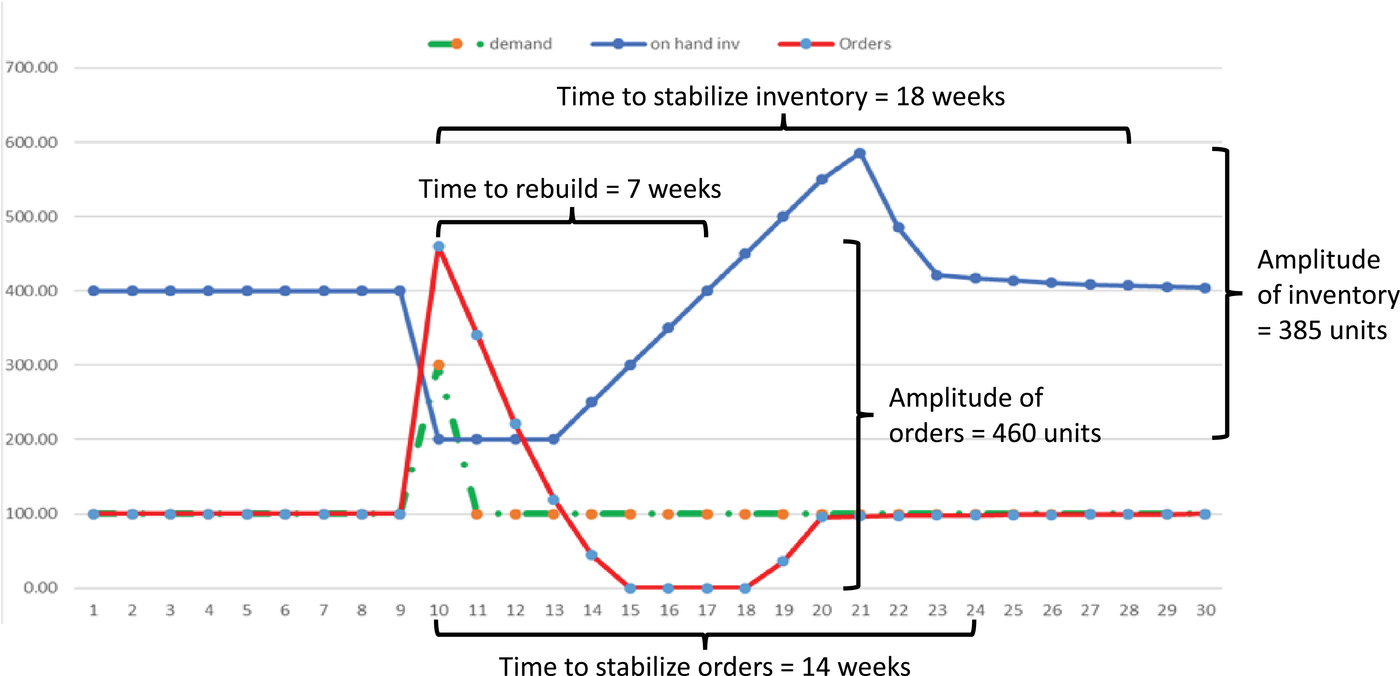
Nevertheless, we can examine the value from being able to defer orders in our simple example. 9 We show in Figure 2 that this helps to mitigate the order amplification. The order amplitude now is only 128 units, as the orders are capped at the start capacity. The time to stabilize the orders, however, is still long, taking 14 weeks. There is less improvement to the inventory dynamics. The time to rebuild is still 7 weeks, the inventory again overshoots, peaking at 550 units after 10 weeks, and the time to stabilize the inventory is again 18 weeks. The inventory amplitude is now 350 units.
One‐time surge: α = 0.20, deferred ordering
Sustained increase in demand
For the second ground truth, we suppose that demand spikes to 300 in week
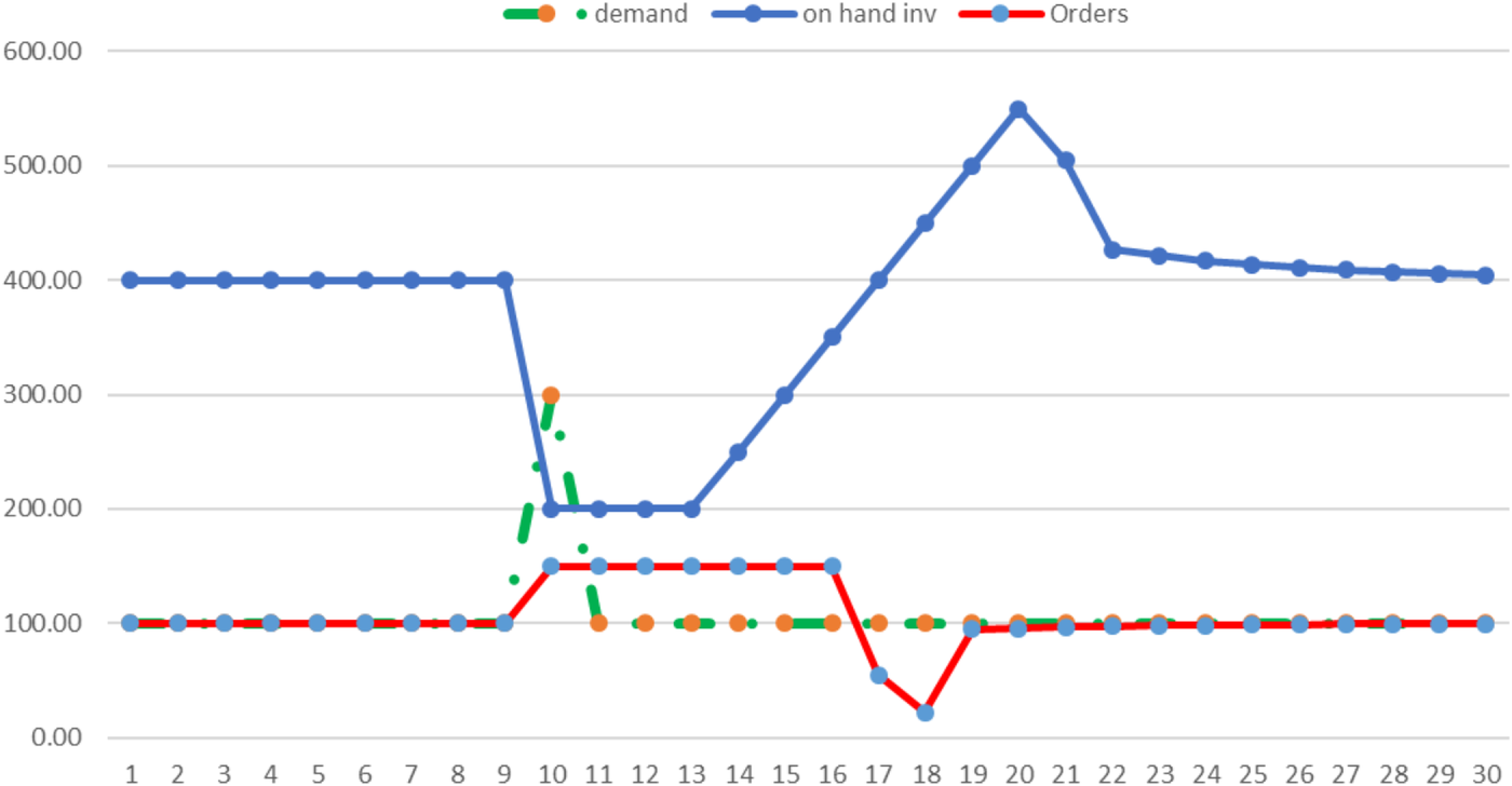
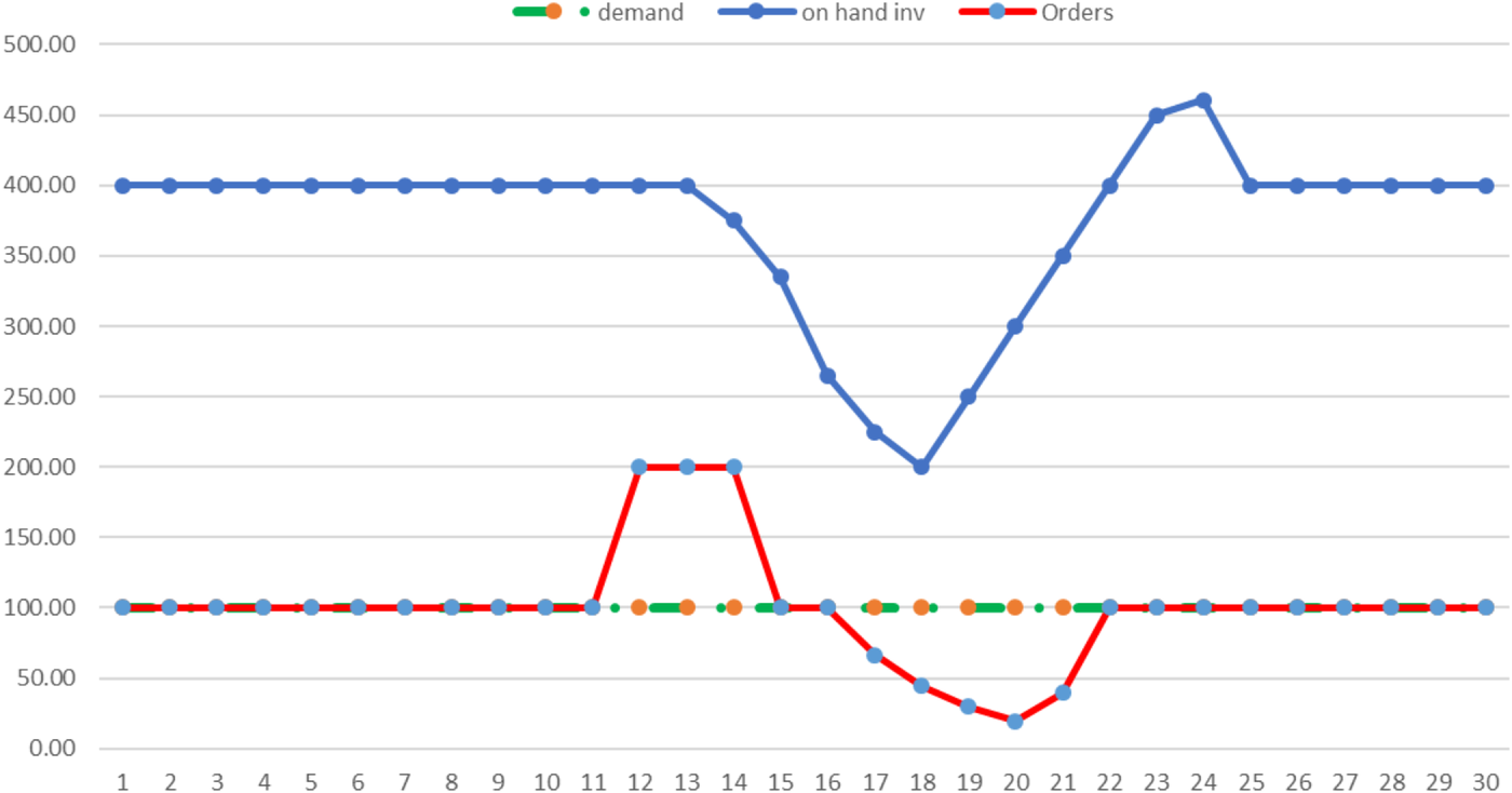
We show in Figure 3 the system behavior with a smoothing parameter of α = 0.20 for the forecast model, for comparison to the prior cases; this parameterization corresponds to the store thinking that most of the spike is likely a one‐time aberration.
Sustained increase in demand: α = 0.20
The dynamics for this case have a similar structure to that in Figure 1: The demand disruption generates an order and inventory wave that are amplified; but the lengths of the waves are much longer. The order amplitude is the same at 460 units: The spike triggers a large order in week 10, and orders eventually drop to zero. However, for this case, the orders remain around 450 for 4 weeks as the store recalibrates its demand forecast, recognizing the increase in demand, and as the supplier lead‐time grows due to the large orders. When demand returns to 100 in week 14, the store cuts its forecast and orders. These cuts continue as demand remains at 100, and by week 17, the store stops ordering as it projects a surplus of inventory on order. Indeed,
The demand over the weeks 10 to 13 totals 750 units, which reduces the inventory down to 50 in week 13. Demand then drops back to 100, and the store starts to rebuild its inventory at a rate to 50 units per week; it then takes an additional 7 weeks to return to 400, and the time to rebuild is 10 weeks.
However, the inventory overshoot in this case is now enormous. In response to the demand of 750 units over weeks 10 to 13, the store orders nearly 2000 units. The inventory then increases to a peak of 769 units in week 28,
These dynamics from this demand event are quite revealing. The increase in demand over a 1‐month period disrupts the supply chain for over 5 months. If the store had used a more responsive forecast model (larger smoothing parameter), it would have overordered even more and the time to stabilize would increase to 6 months. For this case, surprisingly, the best response comes when the store assumes the demand increase is transitory, and uses a smoothing parameter α = 0. In this case, the inventory amplitude is 400, with inventory peaking at 450 after 11 weeks; the time for orders to stabilize is only 10 weeks or 2.5 months. Yet, it is hard imagine that the store could keep its forecast at 100 units per week after seeing a month of substantially higher demand.
SUPPLY CHAIN PHENOMENA: SUPPLY EVENTS
In addition to distorting the demand in many supply chains, the pandemic disrupted the supply side. There were many reasons for these supply disruptions, which resulted in reduced capacity, reduced product availability, and longer lead‐times.
In many manufacturing and logistics operations, supply was constrained by labor availability and/or inflexibility. In effect, labor became the bottleneck in these operations, and this bottleneck tightened for a couple of reasons: due to safety protocols that required social distancing in the workplace, and hence reduced line speed or throughput; due to absences because of illness, quarantine provisions, fear of illness, closed day care, and/or closed schools.
In addition, the labor supply contracted due to the Great Resignation. Many workers left the labor force for various reasons, such as extended unemployment benefits as well as Covid fear. It remains unclear at this time how much of this labor force reduction is transitory and how much is permanent. Nevertheless, this has affected manufacturing and transportation operations, with uncertainty as to how long it will persist. Inevitably, the tightening of supply increased the lead‐times for manufacturing and transportation links in supply chains, and resulted in shortages.
Furthermore, the pandemic made apparent the fragility of our supply chains. A common proverb (which predates by centuries any notion of a supply chain) is that “a chain is only as strong as its weakest link.” A supply chain is a network of links, and often several supply chains will share a single link. As a consequence, a single link failure can have an impact on a huge number of disparate supply chains. For instance, the short supply of semiconductors has created a shortage for new vehicle production as well as delays in the launch of new electronic devices. The West Coast port constraints have extended the lead‐times for all imports from Asia, from Christmas toys to auto parts.
The pandemic highlighted an inflexibility in many supply chains to reallocate supply to different channels as demand changed. One of the most visible examples was the food supply chain, when institutional demand dropped and the supply chain struggled to divert its supply to the consumer channel. Another example was when offices closed and staff worked at home, and the supply chain for office supplies needed to make a similar reallocation.
SIMPLE MODEL ON SUPPLY CHAIN DYNAMICS: SUPPLY EVENTS
Similar to demand events, we use a simple numerical model to examine the impact of these supply events and to characterize the system dynamics. The model setup is the same as for the demand events. We consider a store that sells a staple like toilet paper with stable demand at 100 units per week. The store replenishes weekly from a supplier with a reliable lead‐time of 4 weeks.
We assume the store operates with an order‐up‐to policy, exactly as described above for the demand event cases. The store experiences constant demand of 100 per week, and its forecast remains at this level throughout the supply event.
We assume that when a supply event commences, the supplier knows exactly the duration and extent of the supply event. The supplier then can project what its lead‐time will be for orders placed in the following week. 10 The supplier shares this information with the store. The store then adjusts its future order quantities accordingly, reflecting the current lead‐time. This is a conservative assumption, as typically there would be uncertainty in the extent of a supply event, and unlikely that the supplier could or would provide accurate lead‐time updates. In effect, we assume here that the ground truth is known by the supplier, and the supplier shares its consequences with the store.
We consider two stylized supply events. In the first case, the supplier shuts down and has no capacity for 3 weeks. In the second case, the supplier has a capacity reduction and has reduced capacity over a 5‐week period. All other model assumptions are the same as for demand event examples.
Supplier shutdown
The supplier loses its start capacity in weeks
We show in Figure 4 the system behavior. We note that the smoothing parameter for the store's forecast is not relevant here, as demand is a constant at 100 per week.
Supplier shut down for 3 weeks
The supply event, as witnessed for the demand events, triggers an order wave and an inventory wave. The shutdown increases the supplier lead‐time from 4 to 6 weeks, which prompts the store to order 300 in week 11. This increases the lead‐time even more, which results in continued overordering by the store in the next 2 weeks. Once the shutdown ends, the lead‐time returns to 4 weeks, the store recognizes the overordering and cuts its orders. The order amplitude is 288 units, and the time to stabilize the orders is 12 weeks.
The 3‐week shutdown drops the inventory from 400 units to 100; after the shutdown the inventory recovers at the rate of 50 units per week, with the time to rebuild also being 12 weeks. However, the inventory then overshoots the target, reaching a peak of 478 units in week 24, for an inventory amplitude of 378 units. The time to stabilize the inventory is 15 weeks.
Supplier slowdown
The supplier has reduced start capacity of 75 units in week 10, 60 units in week 11, 30 units in week 12, 60 units in week 13, and 75 units in week 14. This slowdown might be the result of labor shortages, or Covid‐related restrictions, or raw material shortages from the supplier's supplier. We show the system behavior in Figure 5.
Supplier slowdown over 5 weeks
The dynamics are quite similar to those for the
SOME OBSERVATIONS AND LESSONS
The pandemic has brought innumerable demand and supply events upon supply chains that are much, much more complex than our numerical examples. In this section, we provide some observations on some of these real‐world supply chain phenomena and where applicable, relate to the findings from the numerical examples. Admittedly, in our examples, we have ignored many complicating factors like uncertainty, human behavior, limited information, and political considerations, let alone the overall network complexity of real‐world supply chains. Nevertheless, we think there are some useful lessons that emerge from the experiences over the past 2 years, and our examples might shed some light on a few of these.
The beer game is alive and well
At the onset of the pandemic, with the lockdowns, we experienced hoarding of essential items like masks, hand cleansers, and toilet paper. This demand spike resulted in shortages, which led to panic ordering, exacerbating the shortfall. The supply chain responded as quickly as it could but with delays due to its transit and manufacturing lead‐times. In many cases, the supply chain overestimated the extent and duration of the demand spike, and overproduced, creating an inventory surplus. These supply chain dynamics were no different from what we witness in the beer game (Sterman, 1989), and illustrate with the
The semiconductor shortfall is another example of the beer game at work. At the start of the pandemic, the industry seemingly observed a short‐term drop in demand. With the lockdown, there was an even greater slowdown in production, which depleted the inventories. In addition, the industry seems to have reduced its demand forecast, expecting the lockdowns to slow economic growth and consumer spending. This then prompted a delay in capacity expansion, in an industry that tries to keep its capacity slightly ahead of the total market demand (due to the enormous capital cost for capacity). When demand recovered, there was neither enough inventory nor capacity; and with the long lead‐times to increase capacity, it may be some time before capacity again reaches the market demand. Until then, there will be shortages and delays. This seems to be a combination of a delayed demand event (
Vulnerability of long supply chains
The length of a supply chain can be expressed in terms of its lead‐times as well as the number of stages or links. Both dimensions can contribute to the vulnerability of a supply chain. The more links, the more exposure there is to something breaking or being disrupted, particularly if the links are geographically dispersed. Furthermore, the more links, the harder it can be to find or uncover the critical link(s) or bottleneck(s) that constrains a system that is under stress. As apparent from our examples, longer lead‐times result in greater dynamics when there is a demand or supply event. The length and amplitude of the waves depend directly on the lead‐times. We also saw amplification from one supply stage to another; from research on the bullwhip, we know this amplification typically continues up a supply chain. Hence, a disruption triggers longer lasting instability across a supply chain with more stages and longer lead‐times.
Cost of long lead‐times
Product companies have created long supply chains in the pursuit of low cost, where the low cost is largely attributable to lower manufacturing costs. Yet, in making these decisions, we contend that these companies have underestimated the “true” or total costs associated with the length of the supply chain. Most companies recognize that longer lead‐times require that they hold greater safety stock. It is commonly assumed that the amount of safety stock only grows with the square root of the lead‐time; however, this is only true when demand is stationary. The actual required safety stock can typically be much greater when demand is nonstationary, which has become a more valid assumption, especially with longer lead‐times. Furthermore, the pipeline inventory grows linearly with the lead‐times; some product companies understand this, some do not, often depending on who “formally” owns the inventory. In addition, we find that most companies do not fully account for the risk exposure, and more importantly, the cost of inflexibility associated with the longer lead‐times. As noted above, a longer supply chain is more vulnerable to disruption and takes longer to respond or recover from demand or supply events. Our examples provide some insight into how this time to respond depends critically on the length of the supply chain.
Forecasting was challenging
The pandemic itself brought tremendous amounts of uncertainty in terms of how it spread, to what population, and with what impact. There was also tremendous uncertainty in the response, in terms of government regulations and guidelines, as well as government efforts to stimulate the economy. One consequence of all this uncertainty was uncertainty about the impact on the economy. Would the initial dip in economic activity be short term or lead to an extended recession? In light of this macroeconomic uncertainty, it was very hard to predict demand and plan supply.
Furthermore, there were dramatic shifts in consumer demand, mainly due to lockdowns. With families at home, demand for home furnishings and home improvement supplies surged. Yet, with families not traveling, demand for vacation‐related products and services dropped dramatically.
During normal times, inventory and production planning are often based on a demand (or supply) forecast that is captured by a point estimate (e.g., average demand) and a measure of uncertainty (e.g., standard deviation or confidence interval). Such a forecast suggests a high degree of continuity or smoothness to the possible demand outcomes. As discussed above, during the pandemic, the possible demand outcomes were oftentimes dramatically different depending on which scenario materialized. In a world with such dramatic uncertainties, scenario‐based forecasting and operational planning are required.
Lean was not the culprit
Many pundits asserted that the supply chain shortages were due to lean practices, and that the fix is just to hold more inventory. Possibly, in a few instances, this might have helped; for instance, a strategic buffer of toilet paper might have handled the temporary demand spike in the first week or two of the pandemic. Nevertheless, we cannot imagine that this could be justified on a cost–benefit trade‐off. In other instances, where there was a more enduring mismatch between supply and capacity, an inventory buffer would have, at best, just provided temporary relief. And such an inventory buffer is not costless. First, there is the traditional cost of holding inventory. In addition, an inventory buffer can hide system events, such as an increase in demand or a drop in capacity; in this case, the inventory might delay the recognition of such events, which then delays any responses.
A characteristic of a lean system is that it is responsive. This means that inherently it has a short lead‐time (or response time), and has some limited capability (i.e., some slack) to handle variation in supply and in demand. These features suggest that a lean system with short lead‐times and some slack is better suited to managing through unsettled times, like the pandemic.
IMPLICATIONS FOR OPERATIONS MANAGEMENT
We conclude with some suggestions of important topics and opportunities for our community. Our general theme is that we need to pay more attention in our research and teaching on the design and planning of supply chains for “non stationary” times. Traditionally we make assumptions in our supply chain models of a steady state and/or deterministic future. Yet, we anticipate that such assumptions will become increasingly less relevant in the future. Indeed, in the past 2 years, it has been impossible to forecast demand and/or supply in many supply chains. Whereas we expect and hope that the future brings back more normalcy, we expect to continue to see nonstationarity in both demand and supply. On the demand side, this nonstationarity equates to an inability to forecast demand. This difficulty may be due to economic cycles, product life cycles, marketing tactics, availability, and consumer behavior. On the supply side, this nonstationarity arises from the complexity of our current supply chains. Many interdependencies arise from this complexity, which results in supply chains being fragile and readily broken or disrupted.
Better understanding of supply chain resilience
Supply chain resilience has been a vibrant research topic for some time (Simchi‐Levi et al., 2015; Tomlin, 2006), yet this topic remains of great interest and critical importance. There are opportunities to improve how we define and measure resilience, how we assess the resilience of a supply chain (including stress testing), and how we build resiliency into a supply chain (e.g., dual sourcing, flexible resources and processes, strategic inventory, surge capacity, contracting). We also need better ways to assess the total costs and benefits from these tactics, including the value of having a shorter supply chain.
Better response to shocks and disruptions
As evidenced throughout the pandemic, a demand spike or supply interruption can create havoc in a supply chain. We conjecture that one reason for this is due to ineffective responses to these shocks, as seen with our numerical examples. It is clear that following a textbook model does not work, and we need to develop better ways to “play the beer game” in real life. One might develop models that are better attuned to these nonstationary conditions and that have a better toolbox from which to provide robust tactics and solutions.
Role of government
Over the course of the pandemic, the government intervened on occasion to protect national interests. For instance, for some scarce critical products, like medical supplies and equipment, each country took steps to prioritize its domestic needs first. In light of these recent experiences, one might examine the role of government in assuring the functioning of critical supply chains (e.g., medical equipment, health supplies, food, energy). Should the government hold stockpiles of critical products? What is the role of government in developing and overseeing any stress testing of an industry supply chain? Can the government create and administer an information infrastructure necessary to facilitate allocations of critical supplies at times of shortages?
The U.S. government played an absolutely essential role in the vaccine development by placing advanced purchase orders; this effectively was a risk‐sharing contract that transferred much of the drug‐development risk from the drug companies to the government. Under what circumstances should the government make similar interventions into the workings of the private sector? Where else would it be socially economic for the government to off‐load some of the risk borne by industry, and how?
Online commerce
The pandemic has accelerated the transition to online commerce, raising its importance and criticality. Research directed at improving and optimizing the supply chains for online retailers remains a rich opportunity for our community.
Better understanding of supply chain capacity
Over the pandemic, we witnessed many supply chains that could not keep up with demand, resulting in long lead‐times and shortages. Yet, it was not always clear what the capacity was for a supply chain, or how to measure it. One can often associate a capacity with a node or link in a supply chain (e.g., a transportation arc or manufacturing step). Yet, these nodes and links are typically shared across several supply chains. An open question is how to think about and evaluate the capacity in a supply chain, given the inherent complexity and interdependencies. This would seem essential in order to understand how a supply chain responds to a disruption, or how quickly it can scale to meet increased demand. Furthermore, many of the tactics for increasing the resiliency of a supply chain equate to adding reserve capacity and/or making capacity more flexible at a node or link. The cost for such tactics can be enormous; in most contexts, it is very expensive to have idle capacity. To justify such costs, it will be necessary to evaluate the benefits, which requires understanding how slack capacity at a supply chain node or link augments the capacity of the relevant supply chain. In theory, the cost of reserve capacity might be more tolerable if excess capacity can be shared across multiple firms; however, in practice, the benefit of sharing is questionable if the firms all want to call on it at the same time.
Footnotes
ACKNOWLEDGMENTS
The authors are honored to be included in this issue that celebrates the 30th anniversary of POM and wish to thank the editors Chris Tang and Subodha Kumar for their kind invitation to participate. The authors are also grateful for the helpful and constructive feedback provided by the editors on an earlier version of the paper.
1
2
For instance, the challenges faced by Abbott Laboratories are described in a
3
As this is a discrete time model, the actual lead‐time is integer. For the orders placed in week
4
In their noteworthy work on supply chain resiliency, Simchi‐Levi et al. (![]() ) introduced “time to recover” as a parameter that specifies how long it takes a supply chain node to recover after it has suffered a disruption. Our time‐related measures are inspired by this, but have been tailored for our simple model. Time to rebuild is the initial time to recover the inventory, while time to the inventory or orders is the time to fully recover.
) introduced “time to recover” as a parameter that specifies how long it takes a supply chain node to recover after it has suffered a disruption. Our time‐related measures are inspired by this, but have been tailored for our simple model. Time to rebuild is the initial time to recover the inventory, while time to the inventory or orders is the time to fully recover.
5
With the assumed exponential smoothing model, the orders will gradually approach the equilibrium order rate of 100 per week; we set the time to stabilize (TTS) the orders to be when the store orders get to within 2% of this value, that is, when orders remain within the interval (98, 102). Similarly, the inventory TTS is when the inventory remains within 2% of the starting value of 400.
6
We have implemented the model in a spreadsheet, which is posted as Supporting Information to the paper.
7
With smoothing parameter α = 0.20, the spike of 300 increases the weekly forecast by 40 from 100 to 140; the demand increase of 40 increases the order‐up‐to point by 160 (4 weeks × 40 units/week). Hence, the order is the demand (300) plus the change in the order‐up‐to (160).
8
![]() might suggest a simplistic prescription that firms should carry excess capacity (difference between capacity and regular demand) to minimize the time to rebuild and TTS metrics. However, idle capacity is expensive and it may not be economically viable to carry that capacity. An alternative interpretation of excess capacity is that it is used for other lower priority products until called upon by the primary product. Of course, that means the lower priority products will encounter a capacity loss in such circumstances and will then be subject to the negative transient dynamics studied in the supply event section of this paper. There is no free lunch and supply chain managers need to engage in advance planning to prioritize where the costs will be felt.
might suggest a simplistic prescription that firms should carry excess capacity (difference between capacity and regular demand) to minimize the time to rebuild and TTS metrics. However, idle capacity is expensive and it may not be economically viable to carry that capacity. An alternative interpretation of excess capacity is that it is used for other lower priority products until called upon by the primary product. Of course, that means the lower priority products will encounter a capacity loss in such circumstances and will then be subject to the negative transient dynamics studied in the supply event section of this paper. There is no free lunch and supply chain managers need to engage in advance planning to prioritize where the costs will be felt.
9
For this exercise we assume when the supplier has a backlog, the store places its “desired” orders in a virtual queue and that the supplier then quotes the current lead‐time based on this virtual queue; however, we now assume that the store can change or cancel any order in the virtual queue prior to its start.
10
More specifically, we assume that at the end of any week, the supplier knows its future start capacity, and knows its current order queue waiting to be started. Thus, it knows the first future week in which it has any unused start capacity; this determines the earliest time when next week's order can start. For example, suppose the supplier loses capacity in weeks 10, 11, 12, that is, it has zero start capacity in those weeks. The supplier learns this in week 10, and receives an order of 100 from the store. This order cannot be started until week 13, but there will still be unused start capacity of 50 units in week 13. Hence, the supplier knows that part of the order that is placed in week 11 can start in week 13; these starts are delivered 4 weeks later in week 17, so the supplier can inform the store that the lead‐time is 6 weeks for the order placed in week 11.