
Abstract
Service‐level requirements play a crucial role in eliminating stock‐outs in a production pipeline. However, delivering a specific service level can become an unattainable goal given the various uncertainties influencing both the production pipeline and customer demand and causing the manufacturer to adapt the initial strategy in response to disruptions. Such deviations from optimality frequently result in unexpected (and potentially very high) costs and are complex to manage. On the one hand, the manufacturer can use a robust or distributionally robust approach to prepare for the worst‐case disruption, ensuring that the realized cost will be lower than the estimated cost with high probability. On the other hand, this solution may lead to overly conservative production schedules. In this article, we take a different approach and develop a bilevel stochastic optimization model with chance constraints, which allows us to make the production more predictable in the event of disruptions by driving costs and optimal schedules closer to the benchmark for each scenario considered. We introduce doubly probabilistic service‐level requirements to account for two interdependent layers of uncertainty, that is, production disruptions and distributional uncertainties in customer demand. This allows us to make high‐quality production decisions with only a limited understanding of the demand pattern. Approximating the problem for a numerical solution, we guarantee tight optimality gaps for high service levels and propose an efficient solution scheme, combining robust scenario reduction with a customized Benders decomposition procedure. In the managerial section, we use the Omega× Swatch MoonSwatches example to demonstrate that a desirable doubly probabilistic service level can be attained for disruptions with a drop in demand. In the case of disruptions followed by a peak in demand, one can tighten the optimality gaps if the service level is reduced.
INTRODUCTION AND LITERATURE REVIEW
Analytical models that incorporate internal uncertainty in the form of a random supply variable into the production optimization process were first studied by Arrow et al. (1958). Manufacturing decisions resilient to production disruptions lead to mitigation strategies with optimized safety stock, risk mitigation inventory, or alternatives for dual sourcing (Chopra & Sodhi, 2004; Lücker et al., 2020; Snyder et al., 2016; Tomlin, 2006). However, one of the main complexities in determining optimal quantities stems from the fact that production disruptions can affect demand (Hendricks et al., 2019; Timonina‐Farkas et al., 2020), driving it either down (e.g., in the case of damage to a manufacturer's reputation) or up (e.g., in the case of unprecedented events such as COVID‐19 or natural disasters). Thus, the production uncertainties and demand perturbations cannot be studied in isolation of each other, particularly in the presence of service‐level constraints (Craig et al., 2016; Katok et al., 2008). Considered as extremes, internal production disruptions cause manufacturers to reduce production capacity (Dong & Tomlin, 2012; Snyder et al., 2016), which, in turn, may influence demand (Craig et al., 2016).
The work of Ciarallo et al. (1994) took an important step forward by combining demand and capacity uncertainties into a single model, in which the demand follows a given probability distribution. However, during a disruption scenario, both demand and its distribution may remain unknown. Manufacturers are frequently unaware of the exact reason for a disruption before it occurs, which causes the results of scenario‐specific customer research to be biased and dependent on distributional assumptions. Nourelfath (2011) extended the literature to the case of robust service‐level requirements, where the probability of meeting a service level was evaluated using Wiener processes and a first passage time theory. From the retailer's perspective, the interdependence between demand and the optimal product assortment was studied in the work of Timonina‐Farkas et al. (2020). In our article, we develop a stochastic cost‐minimization problem with uncertain service‐level requirements extending the literature to the case where demand distributions depend on the realized disruption scenarios. Furthermore, via the notion of a regret function in our model, we control the cost difference between the manufacturer's strategy at the beginning of the planning horizon and its optimal adjustment in the event of a disruption. This also allows to bound the opportunity cost of knowing the disruption scenario a priori. To the best of our knowledge, our model is the first in the literature to combine these aspects and to account for underlying interdependencies, including those implied by random changes in demand distributions.
We propose a bilevel optimization model for determining the production schedule over a planning horizon and introduce doubly probabilistic service‐level constraints that account for two layers of uncertainty. From the manufacturer's perspective, the first layer of uncertainty is caused by the variability in demand and, moreover, the variability in demand distribution. The second layer of uncertainty arises from production disruptions, implying that there is a probability that the service level cannot be maintained. The two types of uncertainty cannot be viewed as independent of one another because production disruptions can originate outside of the firm (i.e., externally) for reasons that are directly linked to demand distribution perturbations (e.g., as during COVID‐19). We account for both types of uncertainty by utilizing chance constraints.
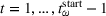
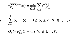
In our bilevel optimization model, the manufacturer addresses the upper‐level cost‐minimization problem and must evaluate the loss incurred under different disruption scenarios. The evaluation of this loss builds on the lower‐level optimization problem, which is dependent on an actual disruption. We introduce the loss incurred under a disruption scenario by means of a regret function that measures the cost difference between a reactive and an anticipative stochastic optimization problem. The anticipative problem optimizes the production strategy of a manufacturer who prepares for a specific production disruption at the beginning of the planning horizon and differentiates between full and partial anticipation. In particular, the manufacturer does not necessarily have the option of conducting customer research to assess the potential demand consequences of the disruption scenario because there could be multiple reasons for the same breakdown. In contrast, the reactive plan assumes that the decision maker only adapts production when the disruption starts. Because the cause of the breakdown is known at the time of the disruption, the manufacturer can estimate possible changes in the demand distribution. Importantly, our regret function contributes to the opportunity cost of knowing about the disruption beforehand. Thus, the benefit of the regret function is its ability to measure the cost impact of different decisions made by the manufacturer, for example, the decision to wait for the disruption before adapting the service level, or preparing for a specific disruption with or without additional customer research.
The resulting bilevel problem is a convex nonsmooth minimum cost network flow (MCF) problem (e.g., Prékopa & Boros, 1991; Zheng et al., 2015). Taking the regret and double probabilistic service‐level requirements into account, we propose an efficient numerical solution scheme that combines a robust scenario reduction approach with a customized Benders decomposition procedure. The solution approach is motivated by the work of Khang and Fujiwara (1993), which is devoted to dynamic minimum cost flow problems without disruptions, while the scenario reduction scheme is inspired by the works of Timonina et al. (2015) and Hochrainer‐Stigler et al. (2019), in which a complex network structure of European river basins is reduced to an ordered list of nodes. Introducing a severity measure and ranking our production scenarios from most to least distant ones according to the robustness principle, we propose an ordered solution scheme with a warm start, which speeds up the Benders decomposition procedure. By approximating the bilevel problem for a numerical solution, we guarantee tight optimality gaps between the initial and approximate problems for high service levels even when the true scenario‐specific demand distribution remains unknown. The guarantees for optimal solution proximity are derived from the results developed by Granot and Veinott Jr (1985), who provide a bound on the distance between optimal solutions of two convex MCF problems. In the managerial section of this article, we demonstrate that the best approximation quality with a desirable doubly probabilistic service level can be attained for disruptions with a drop in demand. In the case of disruptions with a peak in demand, tighter optimality gaps can be guaranteed if the service level is reduced. Our model encompasses a variety of practical applications due to the fact that our solution method is gradient‐free and, thus, a zero‐order method.
This article is organized as follows: The theoretical framework is developed in Section 2. First, the initial model and its approximation are presented for the case without disruptions, followed by a description of the extension to production disruptions with uncertain demand distributions. In Section 3, we develop the robust scenario reduction scheme and present a customized Benders decomposition with novel feasibility cuts and warm‐start techniques. In Section 4, we demonstrate the managerial implications of doubly probabilistic service‐level requirements in the optimization problem with production disruptions.
MATHEMATICAL MODEL
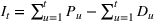
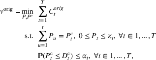
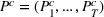
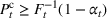
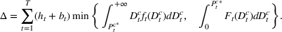
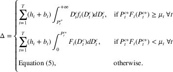
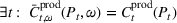
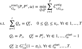
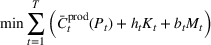
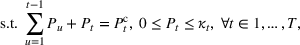
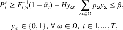
Consider a manufacturer deciding on the production quantity


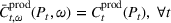
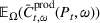
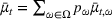
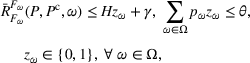
Next, we let Let


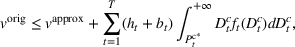
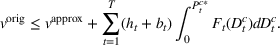
To prove this theorem, we note that the feasible regions of problems (1) and (2) coincide. Therefore, the first statement of the theorem is a direct consequence of Jensen's inequality for convex functions, and it also results from two lower bounds stated in Appendix A.1 in the Supporting Information. To derive the upper bounds, we consider an optimal flow


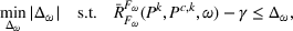
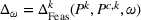
The upper bound (3) is tighter than the upper bound (4) if


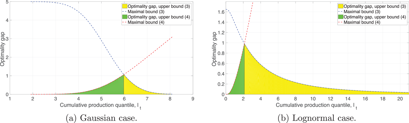
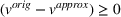
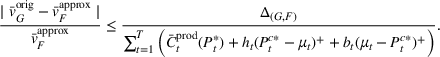
Bounds for the optimality gap
As expected, the optimality gap is bounded tightly for cases with high or low service‐level requirements. The bound is least tight at point

Production disruptions
In this section, we extend the initial model (1) and its approximation (2) to the case of production disruptions and distributional perturbations in demand. The discrete set of all production disruptions is denoted by Ω, while each particular scenario is denoted by


When faced with the risk of disruptions in the production pipeline, the manufacturer wishes to keep the production economically resilient. On the one hand, one can rely solely on a single‐level minimization of the expected total cost, taking disruption scenarios into account. In this case, if a disruption occurs, the manufacturer must adapt its strategy and react to the disruption in order to meet demand. By doing so, the manufacturer deviates from the expected optimum and observes the realized (and possibly very high) cost dependent on the disruption scenario. On the other hand, the manufacturer can use a robust or distributionally robust approach to prepare for the worst‐case disruption, ensuring that the realized cost is lower than estimated with a high probability (Ben‐Tal & Nemirovski, 1988, Nourelfath, 2011). Nevertheless, this solution may be overly conservative. In addition to these methods, there is another option that has not yet been well represented in the literature. In particular, the manufacturer can constrain the difference in optimal costs between (i) the strategy that can be implemented immediately in response to a disruption and (ii) a benchmark, which is an idealistic, but not realistically implementable, optimal production schedule. Under conditions of Lipschitz‐continuity of the cost functions, this approach bounds the difference in optimal production schedules between the above‐mentioned strategies, making the production more predictable by driving the schedule closer to the benchmark for each disruption scenario. Moreover, as we demonstrate further in this article, the cost difference between the production schedule implemented in normal times and the reactive strategy is also bounded in this case.
Overall, we control pair‐wise differences in costs between the following strategies:


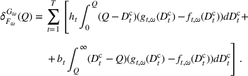
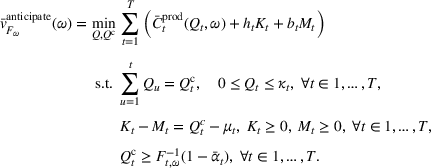
Given the reactive and anticipative setups (8), (9), and (10), we state the bilevel cost‐minimization problem (11) with the stage‐wise objective

We note that the objective function of problem (11) is equivalent to the function


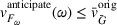

Overall, the scenario‐specific differences in costs between anticipative and reactive strategies can, therefore, be bounded as schematically shown in Figure 2, where we introduce the notion of regret functions


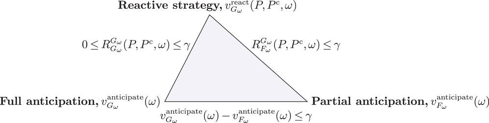
Bounded regrets
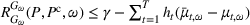
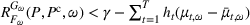
Importantly, the regret


High service‐level requirements and the regret reduction
Next, we demonstrate that high service levels play a crucial role in reducing regrets beyond the threshold γ. For this, we introduce the cost misfit implied by the difference in holding and backlogging amounts due to distributions


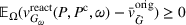
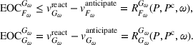
Expected opportunity costs (EOCs) and the regret reduction
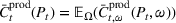
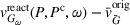
Further, before we proceed with the approximation of problem (11), we analyze the potential loss incurred by a decision maker whenever a disruption scenario ω occurs. For this, we account for expected opportunity costs (EOCs) (i.e., forgone benefits) of anticipative strategies (9) and (10) with respect to the reactive strategy (8). In particular, the EOC of knowing about the production disruption is defined as the difference in the manufacturer's profits between the anticipative (i.e., foregone) and reactive strategies. Though problem (11) is a cost‐minimization problem, its optimal solution coincides with the decision in the corresponding profit‐maximization problem if the total revenue from sales depends on the uncertain demand rather than production quantity (see Appendix A.2 in the Supporting Information). As a result, the EOCs of fully and partly anticipative strategies (denoted by


It should be noted that, similar to the opportunity cost, the regret function


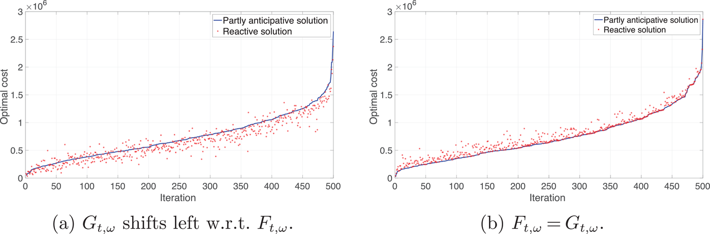
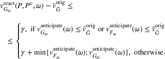
Possible optimal values of the anticipative and reactive problems
It is also worth noting that the probability of negative regrets should not be constrained because they reduce EOCs and appreciate the ability to respond to an upcoming disruption at a lower cost than preparation in advance would allow. This is also why the mirror constraint
Approximation for numerical solution
The optimal solution of (11) is called a resilient plan for problem (1). Our goal is to accurately and efficiently develop such a plan in the absence of complete knowledge about distributions


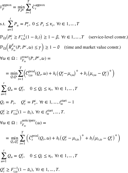


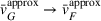
Optimization problem (15) constitutes a bilevel decision‐making program because the regret function form is dependent on the reactive solution. In contrast, the anticipative problem is a single‐level optimization problem that can be solved efficiently for all scenarios. To constitute a fine approximation of problem (11), the optimal solution of (15) must (1) be feasible in problem (11) (see Proposition 1) and (2) provide a tight optimality gap on the optimal value of problem (11) (see Theorem 2). Under the condition of Lipschitz‐continuity, the latter also implies a small difference in optimal solutions of problems (11) and (15). With a small abuse of notations, let


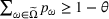

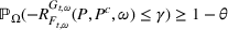
See Appendix A.3 in the Supporting Information for the complete proof and note that by increasing the set of scenarios Ω, the manufacturer increases the probability of finding its subset


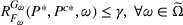


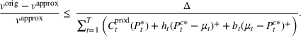
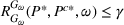
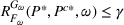
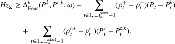
Let the conditions of Proposition 1 be satisfied. Denote by (Lower Bound) The lower bound on the original problem (11) yields (Upper Bounds) The following upper bounds (denoted u1 and u2) hold: The optimality gap (Relative Error) The relative error of the approximation follows from statement 2, that is,


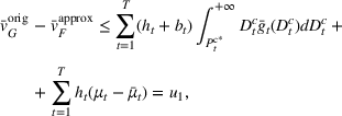
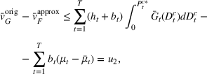


See Appendix A.4 in the Supporting Information for the complete proof, which is based on the results of Proposition 1 and proceeds from stating lower bounds for the problem's objective function to its upper bounds.

When Theorems 1 and 2 are compared, one can see that the upper bounds and optimality gap in the case of production disruptions have additional terms due to the difference in demand distributions. These terms describe the deviation of production quantiles in the perturbed distribution.
Further in the article, we consider the following two cases:


Case 1 is described in Theorem 2 and guarantees the existence of the upper bound for the optimality gap given the set of scenarios


SOLUTION METHOD
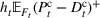
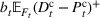
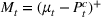
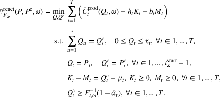
We introduce the inventory level


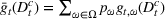
Here, demand distributions


Next, the lower‐level optimization problem (22) arises because the reactive setup in the regret function


Scenario generation
We consider the following three uncertainty types influencing the production pipeline:

We let


Probability of production disruptions with different disruption lengths (
The steady‐state probabilities of this Markov chain are unique due to the well‐known Perron–Frobenius Theorem for nonnegative irreducible transition matrices. We let ξ0 be the steady‐state probability of no disruption and


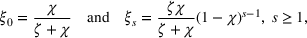


Given


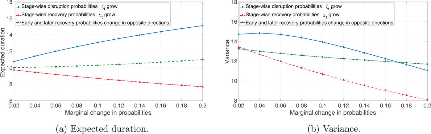
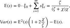
Expected duration and variance of finite horizon disruptions


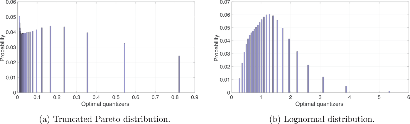
Optimal quantization in the sense of the minimal Kantorovich–Wasserstein distance


The total number of disruption scenarios generated is equal to


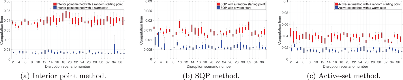
The anticipative solution with the warm‐start and a quadratic production cost function
Bilevel optimization using Benders decomposition
To solve the optimization problem (21a), we apply a generalized Benders decomposition introduced in Geoffrion (1972). A feasible point


Benders decomposition with customized feasibility cuts.
In the next section, we solve problem (21a) using Algorithm 1 and emphasize the following insights: Without knowledge of the true scenario‐specific demand distributions Underestimating the demand and, consequently, requiring a lower service level increases the optimality gap (see Case 2 and the case study on Omega× Swatch MoonSwatches in Section 4). In the setup with production disruptions, service‐level requirements can be kept high by utilizing safety stock. Nevertheless, the difficulty associated with this is that the safety stock grows exponentially for service levels above about 95% (Simchi‐Levi, 2010). The solution to this issue is to produce more during the periods with lower disruption probabilities, or during the periods with disruption scenarios included in the risk budget (i.e., neglected).


MANAGERIAL IMPLICATIONS
In this section, we emphasize the managerial importance of maintaining high service‐level requirements, the fulfillment of which results in accurate production decisions even when estimated demand distributions 


Considering a quadratic production function 
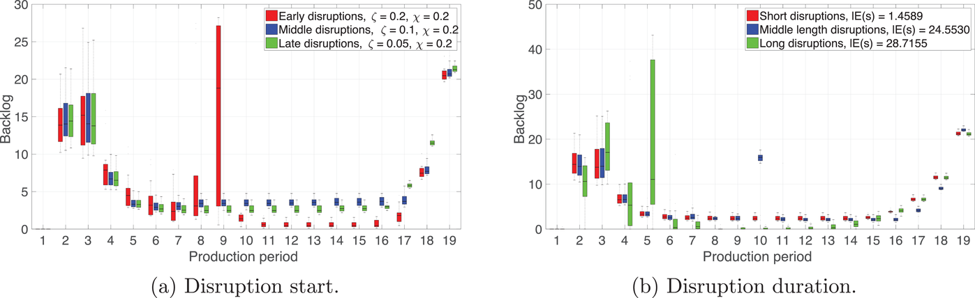
We start by analyzing different types of disruption scenarios and their effects on the optimal production plan. The occurrence and duration of a disruption at time Early disruptions ( Middle‐start disruptions ( Late disruptions (


Furthermore, we distinguish disruptions by their expected duration 


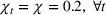

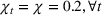


Figure 8 demonstrates the influence of the starting period and the disruption's expected duration on the optimal value of the optimization problem (21a). Figure 8a shows that disruptions with higher probability to start earlier tend to be more costly. This is also consistent with the fact that multiple disruptions are possible over the planning horizon. Furthermore, as demonstrated in Figure 8b, longer disruptions result in higher production costs. Naturally, longer disruptions provide shorter periods of production recovery, putting the manufacturer at a disadvantage.
Optimal values dependent on the expected start and duration of disruptions
Further, Figures 9 and 10 show that the optimal mitigation strategy for scenarios with a high periodic disruption probability 

Mitigation inventories dependent on the expected start and duration of disruptions
Optimal backlog dependent on the expected start and duration of disruptions
As a result, mitigating for such scenarios creates a significant peak in inventory level and necessitates the keeping of a safety stock. Due to the availability of such inventory, the backlog tends to be lower for early and longer disruptions in the second half of Figure 10's planning horizon.
Next, we assess the impact of service‐level requirements on the level of inventory, backlog, and safety stock amounts (Figures 11 and 12). The manufacturer holds more inventory earlier in the planning horizon in order to maintain the same service level as in the absence of disruptions (Figure 11). This matches the behavior of the inventory policy early in the planning horizon in Figure 9. Note that the inventory is at the limit of available capacity (60 units in Figure 11) for service levels approaching perfect customer satisfaction (i.e., beyond 96%). Also, because the safety stock is designed to prevent the majority of stock‐outs early in the planning horizon, its level is increasing in service level given the high probability for early disruptions (Figure 12a). When the service level reaches approximately 95%, the safety stock starts growing exponentially (Simchi‐Levi, 2010).
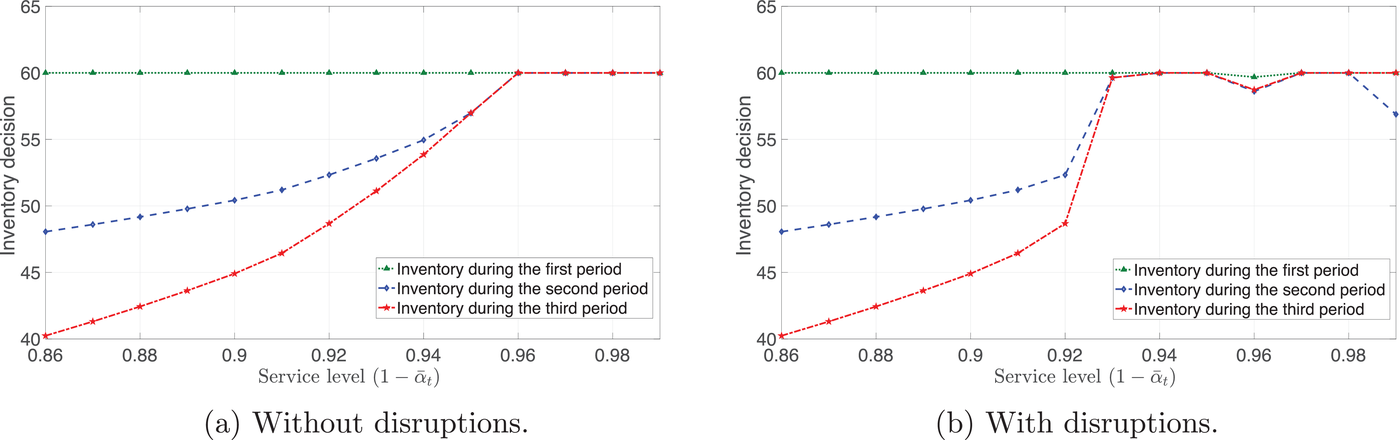
Comparison of optimal inventories with and without disruptions
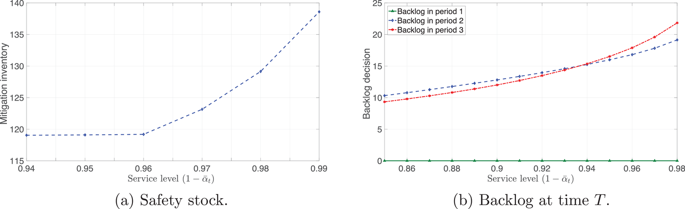
Influence of service‐level requirements on optimal safety stock and backlog amounts
Case study on the Omega × Swatch MoonSwatches
Importantly, we assess the impact of doubly probabilistic service‐level requirements on the optimal cost in problem (21a) using Omega× Swatch MoonSwatches as an example. Eleven new watches devoted to bodies in our solar system (Moon, Earth, Sun, Mars, Mercury, Neptune, Pluto, Uranus, Venus, Jupiter, and Saturn) were released on March 26, 2022, in selected Swatch stores and were followed by a massive and unexpected demand, to the point where Swatch needed to provide clarifications on social media. There could be a variety of reasons for such demand, including the Omega branding on the watches, as well as a price of only US$260 per piece instead of about US$6,600 for the original Omega Speedmaster. Considering the time horizon of 
We specifically consider two layers of uncertainty in the problem: (1) demand variability and (2) production disruptions (e.g., due to a lack of specific color pigments used to produce some of the MoonSwatches), implying that the service level cannot be maintained for some scenarios with probability β. The second layer of uncertainty impacts the service‐level constraint and takes the variability in the unperturbed demand distributions 

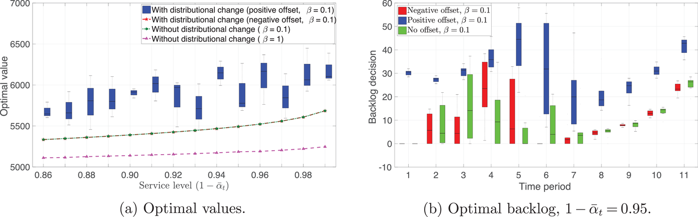
Comparison of optimal values for optimization problems with and without a perturbation in demand
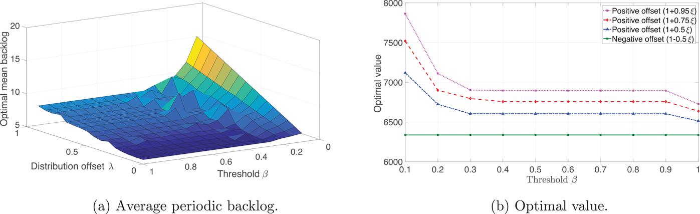
Optimal value and average backlog in the optimization problem (21a) given different demand offsets and risk thresholds
As shown in Figure 13a, a negative multiplier λ, implying that a lower production should suffice for the demand, results in a tight optimality gap for the problem (21a) with a fixed probability threshold β. This is in line with Case 1 described in Section 2. Conversely, a positive multiplier λ results in a larger optimality gap and, thus, an underestimation of total costs for a given service level. This is the case for Omega× Swatch MoonSwatches, for which the demand was initially underestimated and described by Swatch as “phenomenal” when observed. Note that the size of the optimality gap and, thus, the cost increase is dependent on the quantile offset and increases on average for higher service levels (see Case 2 and Figure 14a, where the optimal cost reaches about US$24,500 for the average demand of 60 pieces per store and a service level of 99%). Moreover, as demonstrated in Figures 13b and 14, larger‐than‐expected backlogs resulting from demand underestimation and a lack of safety stock may remain unresolved until the end of the planning horizon if no additional actions, such as changing the pricing strategy or expanding the production, are taken.
In conclusion, we numerically test the sensitivity of the results to changes in the demand distribution mean. We observe that the growing mean demand naturally increases the necessary level of safety stock (Figure 15a), backlog in later time periods (Figure 15b), and, thus, the lost sales at time T. In the Omega× Swatch case and in the absence of sufficient safety stock, optimal backlog plays an important role due to the fact that a large portion of customers are willing to return and purchase the watch for US$260. Nevertheless, Swatch will have to reevaluate their long‐term decision, which could include limiting the edition or increasing the price to control demand.
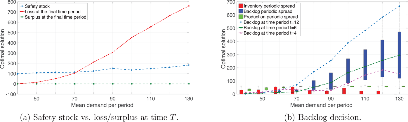
Influence of mean demand on the optimal strategy
CONCLUSION AND OUTLOOK
Optimization models accounting for production uncertainties and capable of determining resilient strategies are crucial for the mitigation of supply chain disruptions. In this article, we account for two layers of uncertainty that affect the production pipeline. The first layer results from the variability in demand and demand distribution. The second layer is triggered by production disruptions, when the service level cannot be maintained with some probability. We develop a bilevel optimization model that takes both demand uncertainty and production disruptions into account by using chance constraints and doubly probabilistic service‐level requirements that incorporate the dependence of demand distribution and production disruptions. Our approach is particularly advantageous for manufacturers who wish to build resilient production strategies that do not require significant adjustments in the event of a disruption. Even though the manufacturer has the option of focusing solely on lowering the expected total cost, the corresponding optimal strategy would need to be adjusted in the event of a disruption. By doing so, one deviates from the expected optimum and observes the realized (and, potentially, extremely high) cost dependent on the disruption scenario. Clearly, the manufacturer can use a robust framework and prepare for the worst‐case disruption guaranteeing that the realized cost is lower than estimated with a high probability. Nevertheless, this solution may be overly conservative. Aside from these options, there is one more possibility that we address in this article. Naturally, the manufacturer can constrain the difference in optimal costs between a strategy that can be implemented quickly in the event of a disruption (i.e., reactive setup) and a benchmark, which is an idealistic, but unattainable production schedule (i.e., anticipative setup). Under conditions of Lipschitz‐continuity, our approach bounds the difference in production schedules between the above‐mentioned strategies, making the production more predictable. The cost difference between the production schedule implemented at the start of the planning horizon and the reactive strategy is also bounded in this case.
Approximating our problem for numerical purposes, we demonstrate theoretically that the optimality gap is tight for high service‐level requirements when disruptions reduce demand. In order to solve the resulting problem numerically, we customize the Benders decomposition procedure by introducing novel feasibility cuts and using warm‐start techniques for computational speed‐ups. In the article's managerial section and by using Omega× Swatch MoonSwatches as an example, we demonstrate that the best approximation quality with a desirable doubly probabilistic service level can be achieved for disruptions with a drop in demand.