
Abstract
We present a new crossing number problem, which we refer to as the edge‐constrained weighted two‐layer crossing number problem (ECW2CN). The ECW2CN arises in layout planning of hose coupling stations at BASF, where the challenge is to find a crossing minimal assignment of tube‐connected units to given positions on two opposing layers. This allows the use of robots in an effort to reduce the probability of operational disruptions and to increase human safety. Physical limitations imply maximal length and maximal curvature conditions on the tubes as well as spatial constraints imposed by the surrounding walls. This is the major difference of ECW2CN to all known variants of the crossing number problem. Such as many variants of the crossing number problem, ECW2CN is

Keywords
Introduction
BASF is the world's leading chemical company (Tullo 2018). It has customers in over 170 countries and supplies about 8.000 products to almost all industries. BASF operates more than 350 sites worldwide, six of them being major, so called “Verbund” sites. The largest site is in Ludwigshafen, Germany, where BASF has its headquarters. The Verbund system is one of the core competencies of BASF; it creates efficient value chains that extend from basic chemicals to high‐value‐added products such as coatings and crop protection agents. In addition, the by‐products of one plant can be used as the starting materials of another.
As part of its Verbund system, BASF operates more than 2.800 kilometers of pipelines in Ludwigshafen. While most of the pipes are dedicated to a certain product or utility, some of them are used for different products alternatingly. To maximize flexibility, BASF operates switching hubs, where dozens of pipes end in the same location, and any two of them might be connected on demand by flexible tubes. The work of connecting and disconnecting pipes was a manual and very unpopular task, due to the weight of the steel pipes and the need for full body safety equipment in the switching hub. However, necessary sub‐tasks, such as leaking test, flushing, and drying made it difficult to obtain an automated solution. Currently, the engineering department of BASF is designing a dual‐arm robotic system to accomplish that task. As the robot is mounted on the ceiling, with its two hands, it cannot remove a pipe crossed by another one. For that, the robot must either remove and rebuild all blocking connections, or release the blocked pipe to the ground, where it has to be removed manually later. Both possibilities impede the efficiency of the system. Thus, the Advanced Business Analytics department within BASF was asked for a mathematical solution of this problem, which translates into a crossing minimal design where the number of blocking connections (so‐called FIFO crossings) is to be reduced to a minimum.
To that end, we are given a two‐layer hose coupling station where units are positioned on two opposing sides surrounded by walls. These units are to be connected by tubes. Figure 1 depicts such a hose coupling station. The connecting tubes (edges) have to obey three physical restrictions (constraints). First, tubes must lie inside the box drawn by the units because the units abut walls. A close distance to the surrounding walls is needed since the fluid flows through units and the tubes emerge from taps integrated in the walls. Due to security reasons, these taps have to be close to the units without any disturbing elements in between, that is, moving the units away from the wall to gain more freedom for tube placement is not an option. Second, the tubes’ length has an upper bound which is imposed by the size of the tube storage. Third, the tubes can only be bent up to a maximal curvature; otherwise, they break. Moreover, the connections between the units change over time, that is, the tubes have to be reconfigured. Possible failure during the disconnection process may cause severe health risks due to leaking chemicals. Therefore, BASF is taking very high safety precautions, like full body protection. In the future, this is supposed to be executed by a dual‐arm robot. As mentioned above, for the robot, crossing tubes pose a challenge and may lead to additional efforts, as all tubes stacked above need to be disconnected first. Therefore, a layout plan for the units, which is crossing minimal with respect to the connecting tubes, is highly valuable.
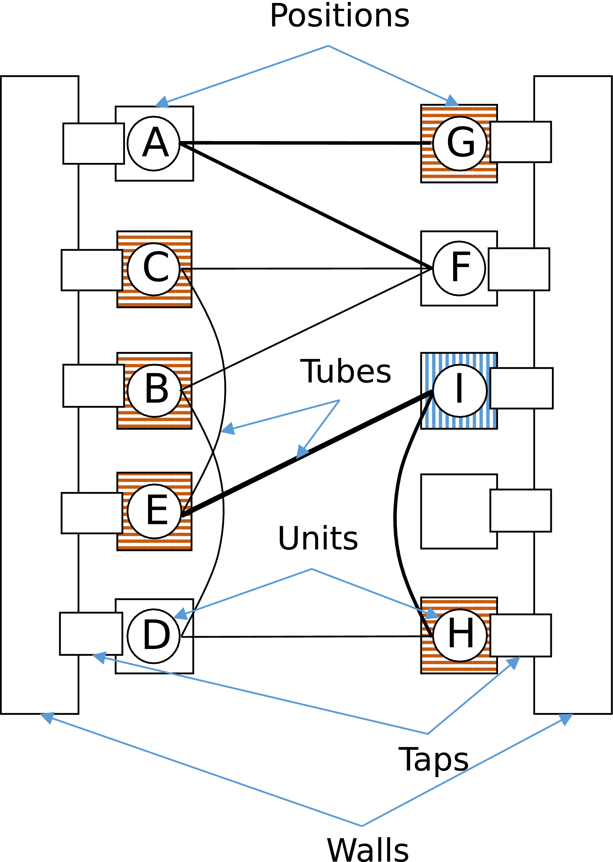
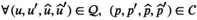
An Illustration of a Possible Assignment of 9 Tube‐connected Units to 10 Positions. Due to the Maximal Curvature Condition, no Direct Neighbors may be Connected and a Maximal Tube Length has to be Respected. This is Illustrated for the Vertically Hatched Position (I) where all Reachable Positions are Horizontally Hatched (B, C, E, G, H). The Thickness of the Edges is Proportional to its Historical Connection Frequency [Color figure can be viewed at
In the real‐world problem at BASF, the locations of 75 units have to be determined. The connections between the units change over time, and we recorded historical connection data over a time span of more than 3 years. Next, we performed a thorough data cleansing in close cooperation with the operating engineering department at BASF and dropped all historical connections which did not generalize well for future considerations. Eventually, we agreed on 375 representative connections whose weights were determined by their historical connection frequency. This leads to a graph with 75 nodes and 375 weighted edges, having an edge‐to‐node ratio of 5.
The available data do not allow a meaningful probabilistic evaluation of possible future connections, because the number of observations is very low compared to the huge number of possible pairings. Consequently, the data are too sparse to extract distributional information, let alone the fact that some sets of pairings exclude each other, while other sets are likely to co‐exist. Therefore, we do not set up a stochastic optimization model. Instead, we separate the problem into a deterministic design optimization problem, which serves as surrogate model, and a simulation problem, that is used for quality evaluation.
The deterministic design optimization problem leads to what we call the edge‐constrained weighted two‐layer crossing number problem (ECW2CN). We formulate this problem as a mixed integer linear program (MILP). The MILP finds an optimal assignment using aggregated data, that is, time independent data, considering both the number of connections between each pair of units and the aggregated connection frequencies. A natural objective function is the minimization of the number of reconfigurations over time which require the removal of FIFO connections. Because our proposed MILP is static, such an objective function cannot be modeled directly. To overcome this challenge, we set up multiple MILPs that differ in their treatments of the weighted edges by employing four different objective functions. Using these four different objective functions, we generate a series of feasible points for the MILP models. These points are then evaluated in a simulation model. This simulation model captures the complexity of the design problem by taking time dynamics and historical connections into account. In a second simulation model, only so‐called FIFO crossings are counted, that is, reconfigurations which require the removal of blocking connections which cause operational disruptions. The best performing point in the second simulation model is then chosen as the optimal design. Computing the FIFO crossings for all feasible points is not possible since the second simulation model is very time consuming.
The ECW2CN is a non‐standard edge‐weighted crossing minimization problem (Schaefer 2020). Because this problem has not been discussed in the literature before, we develop an optimization model and tailor solution techniques to solve this real‐world problem.
Our unique contributions are:
We introduce the edge‐constrained weighted two‐layer crossing number problem (ECW2CN). This is a new variant of the crossing number problem, motivated by a real‐world problem at BASF. We analyze the computational complexity of ECW2CN and present MILP formulations, as well as two tailored decomposition algorithms: a Benders decomposition with direct cut calculation (BDC) and a Dynamic Fix‐and‐Relax Pump (DFRP). The master problem of BDC is strengthened by incorporating some information from relevant parts of the Benders subproblems. These additional cuts are provably stronger than the Benders optimality cuts. All cuts are computed analytically yielding a very efficient algorithm. The DFRP employs the BDC algorithm in a fix‐and‐relax fashion where the problem sizes are dynamically adjusted. This way, DFRP computes high quality solutions while being able to theoretically provide an optimality certificate. We provide a case study using real data of BASF. The real‐world problem is solved by state‐of‐the‐art implementations of all algorithms. Furthermore, final solutions of the real‐world problem for different choices of the objective function are evaluated and compared in a time‐dependent simulation model.
The remainder is organized as follows. We place the ECW2CN problem in the literature in section 2. In section 3, we present a mathematical programming model for the ECW2CN problem and show that ECW2CN is

Crossing Number Literature
The crossing number problem for a given graph G consists of finding a drawing of G, such that this drawing possesses the lowest number of edge crossings (Schaefer et al. 2008, Székely 2004). Many variants of graph crossing number problems have been studied during the last decades. The review paper by Schaefer (2020) lists about 86 different variants. Therefore, we focus our review on important aspects of crossing number problems that are relevant in our context.
The crossing number problem appeared in the 1940s in the context of railway crossing minimization (Turán 1977) and in the 1960s in circuit design (Sinden 1966). However, it took until 2005 for the first exact integer linear programming (ILP) formulations to appear (Buchheim et al. 2005), although, for the related maximum planar subgraph problem, ILP formulations were published a decade before (Jünger and Mutzel 1996a,b. For a general graph G(V, E), the ILP formulation by Buchheim et al. (2005, 2008) models edge crossing via binary decision variables x
e,f
for all edges e ∈ E and f ∈ E. The difficulty lies then in ensuring that a graph exists for given values x
e,f
. This is known as the realizability problem, which is itself an


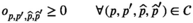
In the literature, a variety of multi‐layer and two‐layer crossing problems are presented. Carpano (1980) discusses two types of hierarchical drawings (also called level drawings): horizontal drawings (nodes are placed on parallel lines) and radial drawings (nodes are placed on concentric circles) in a multi‐layer context. All edges have to be drawn as straight lines, in contrast to general drawing problems where edges can contain bends. The level specification of each node has to be respected. A semidefinite programming approach for hierarchical drawing is presented by Chimani et al. (2012). Hierarchical drawings are extended to allow for intra‐layer connections by Bachmaier et al. (2010); the intra‐layer edges are allowed to bend. With that, Bachmaier et al. (2010) comes close to the ECW2CN problem, when restricting to two layers, which is illustrated in Figure 2. In the ECW2CN problem, we have also a two‐layer set‐up with inter‐layer connections, but the units can be placed freely among the two sides in contrast to Bachmaier et al. (2010). Another similarity of the ECW2CN problem to Bachmaier et al. (2010) is that all edges need to stay inside the rectangle spanned by the location positions. Different to Bachmaier et al. (2010), the ECW2CN problem has restrictions on the inter‐ and intra‐layer connections.
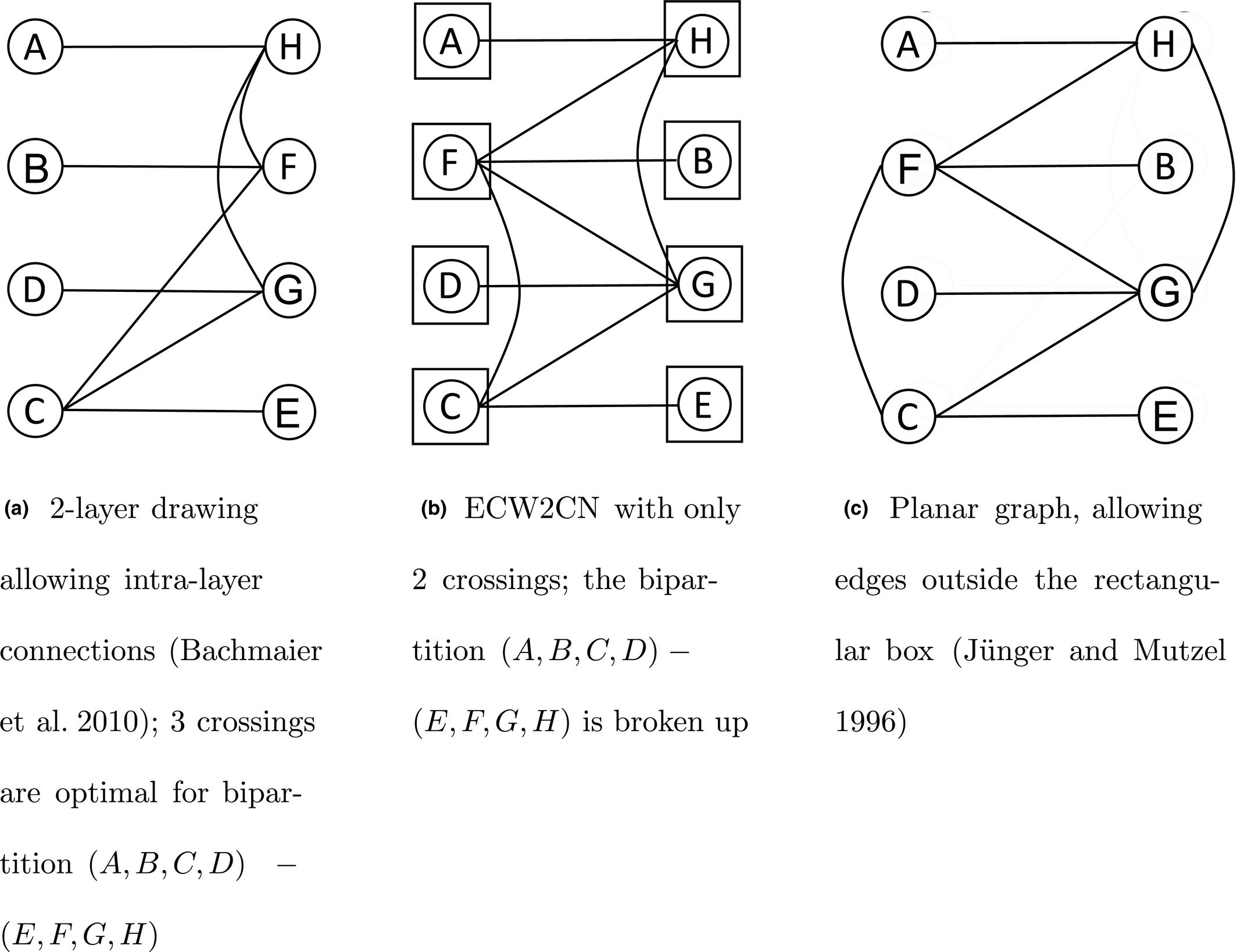
A Comparison of ECW2CN with Related Settings in the Literature, Yielding to Different Number of Minimal Crossings
A special case of two‐layer hierarchical drawings is obtained for bipartite graphs; in the context of multigraphs, Garey and Johnson (1983) call this problem the bipartite crossing number problem. Because only straight lines are allowed for the edges, Jünger and Mutzel (1996a, b) refer to this problem as the two‐layer straight line crossing problem. This is also the usual setting for the k‐layer case where only straight lines are allowed. In the two‐layer straight line crossing problem, the bipartition of the node set has to be respected (hence, there are no intra‐layer edges). An ordering of the nodes, for each of the two layers, determines the graph and its crossings. This allows for efficient permutation approaches (Kobayashi et al. 2014, Laguna and Marti 1999, Palubeckis et al. 2019). As such, the bipartite crossing number problem is highly related to the (quadratic) linear ordering problem (Buchheim et al. 2010, Shahrokhi et al. 2001). Edge‐weighted variants of the bipartite crossing number problem are presented by Çakiro

In sum, ECW2CN has the following key specifications:
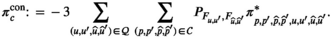
Maximal length and maximal curvature conditions for the tube (that is, edges) have to be met. Though we have a two‐layer set‐up, intra‐layer connections are allowed; like the formulation in Bachmaier et al. (2010). All connections have to stay inside a rectangle spanned by the position locations; similar to the bipartite crossing number problem (Garey and Johnson 1983). Each node (that is, unit u ∈ U) can be placed freely among the two layers; thus, this problem differs from bipartite or two‐layer crossing minimization problems and yields some additional overlapping types, see Figure 3. The edges are weighted due to the historical connection frequencies. However, in contrast to the set up of Kobayashi et al. (2014), weights can be handled in a very flexible framework. In this work, we examine four different manners. The corresponding graph does not have to be connected. Connectivity is a standard assumption as the crossing number problems decompose with their connected components. This is not true for ECW2CN because of the maximal length and maximal curvature conditions. The number of units and places do not have to be the same, that is, there might exist isolated nodes in the corresponding graph. This is a special case of a disconnected graph (see previous point). The “placement” of the isolated nodes is non‐trivial due to the maximal length and maximal curvature conditions. We are facing an edge‐to‐node ratio of 5. Most instances found in the literature have a ratio between 1 and 2.
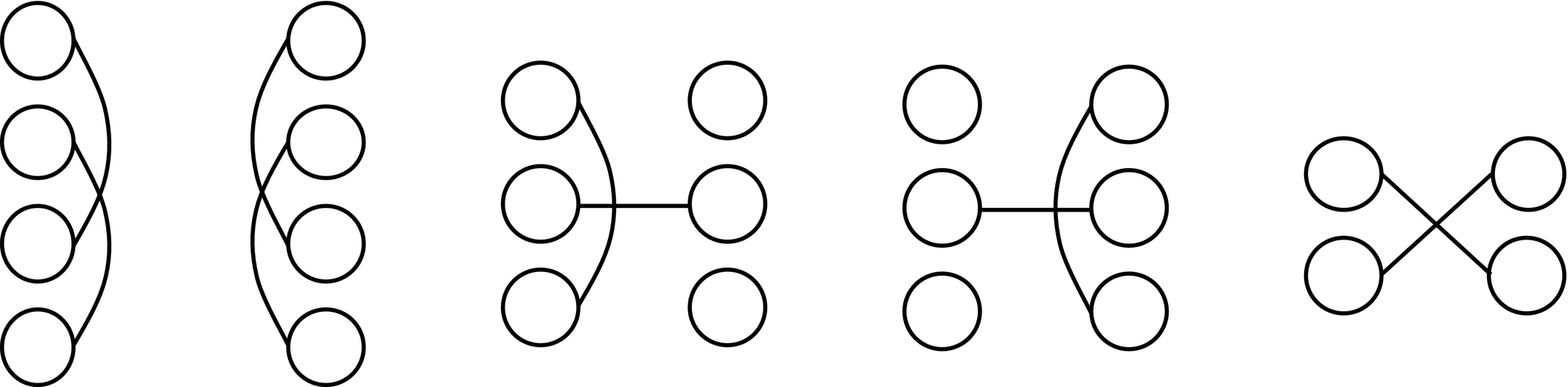
An Overview Over all Different Crossing Types in the ECW2CN
ECW2CN, its Complexity and MILP Formulations
Based on the definition of the ECW2CN in section 3.1, we prove its

The Edge‐Constrained Weighted two‐Layer Crossing Number Problem (ECW2CN)
We begin by defining the notation used in the definition of the ECW2CN as well as in the MILP.
D > 0: Maximal Euclidean distance between two units due to a maximal tube length
E > 0: Minimal distance between two units on the same layer due to maximal curvature


We are now ready to formally define the ECW2CN.
Given is a set of units


ECW2CN is
‐Hard

To show that ECW2CN is

ECW2CN decision version


In our reduction, we use the decision version of the bipartite crossing number (BCN) problem, denoted by BCN‐D.
BCN decision version, (BCN decision version, Garey and Johnson (1983)
We need the following complexity result.
The BCN‐D is Garey and Johnson (1983)

For their reduction, Garey and Johnson (1983) utilize the Optimal Linear Arrangement problem which has itself been reduced from the MAX‐Cut problem in (Garey et al. 1974). Therefore, BCN‐D is

This allows us to state and prove our main result.
The decision version ECW2CN is

Observe that ECW2CN‐D is in

Given an instance of the BCN‐D, that is, a connected bipartite multigraph G(V 1,V 2,E), we construct an instance of the ECW2CN‐D as follows:
D = E = 2


The idea is to use the restriction on the minimal distance between two units on the same layer to ensure that only nodes from V 1 (and V 2) are assigned to the same layer. This can be achieved by assigning any number E > 1 (see below). The transformation is shown in Figure 4.
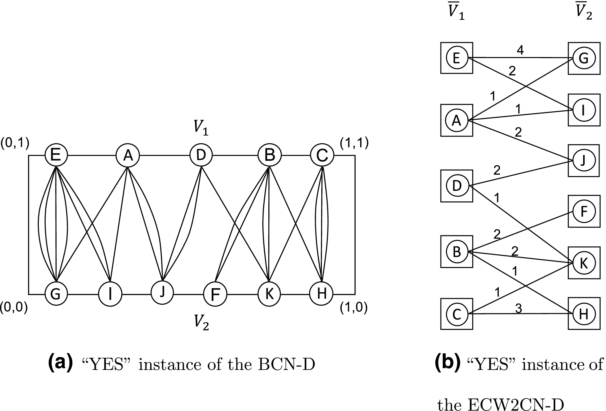
A Transformation of a “YES” Instance for K ≥ 5 of the BCN‐D to a “YES” Instance for C ≥ 5 of the ECW2CN‐D Using the Technique Described in the Proof of Theorem 1
The maximal distance is no restriction as long as

Next, we show that an instance for BCN‐D with bound K is a “YES” instance, if and only if the transformed graph is a “YES” instance for ECW2CN‐D with bound C = K. For that, we observe that both problems count the number of crossings. Thus, if the solution of one problem maps to a solution of the other, then the bounds are the same. It remains to show the existence of such a mapping.
“⇒” Any feasible point for ECW2CN‐D yields a partition of


“⇐” Any feasible point for BCN‐D respects D and E. With that, it is a feasible point for ECW2CN‐D.
The Mixed Integer Linear Programming Models
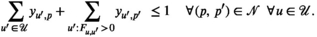
We use the indices, sets, and parameters as introduced in section 3.1. Furthermore, we require the following decision variables


The ECW2CN can be modeled as the following MILP formulation, which we call the monolithic model.
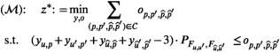

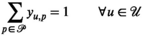
The objective function (1) minimizes the weighted number of crossings. This weighted crossing is modeled through decision variables


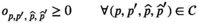
Constraints (5) can be more naturally written as


Nevertheless, constraints (5) are not facet defining for polytope (3)‐(5) as they are dominated by
From the above discussions, we summarize
Formulation

We close this section with a few remarks.
The subsequent theoretical developments do not the depend on a particular choice of the crossing weights, that is, they hold true for all
For illustrative purposes, suppose we have a crossing induced by the positions of (u, u
′) and


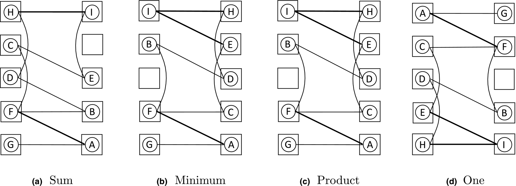
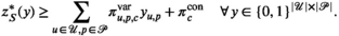
Optimal Configurations of the Graph in Figure 1 with Respect to Four Different Objective Functions
The graph depicted in Figure 1 possesses nine nodes and nine edges whose weights are given by: (A, F): 10, (A, G): 8, (B, D): 6, (B, F): 2, (C, E): 3, (C, F): 5, (D, H): 1, (E, I): 15, (H, I): 12. Depending on the choice of the objective function, we obtain the following optimal assignments as illustrated in Figure 5.
In order to break some symmetry, we extend formulation

Observe that it is possible to reformulate the monolithic model

For our real‐world application, we have


Solution Methods
The monolithic formulation


A Tailored Benders Decomposition with Direct Cut Calculation (BDC)
Benders Decomposition
The idea of Benders (1962) was to separate a, what he called, mixed variables problem into a master problem and a subproblem. The mixed variables in our case are the y
u,p
and the

These constraints are passed onto the subproblem which computes, for a given solution of the master problem (in our case, trial values of variables y u,p ), the objective function value associated with an optimal “response” to y u,p . Exploiting dual information, a feasibility or optimality cut is generated and passed on to the master problem. This way, the master problem is extended by information from the subproblem, in terms of dual extreme directions or extreme points. For a minimization problem, the master problem yields a lower bound and the trial solution together with the subproblem yields an upper bound. By iteratively solving master and subproblems until the upper and lower bounds are sufficiently close to each other, the original problem is solved. This so‐called Benders algorithm always terminates after finitely many iterations because the dual subproblem contains only a finite number of extreme directions and extreme points. For further details, we refer to the literature (Rahmaniani et al. 2017, Rebennack 2016).
For a given trial solution


Notice that


Observe that for given


Let


For some (cut) index c, we define the (variable) cut coefficient

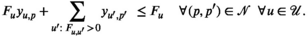
The master problem


For a given cut set


Direct Cut Calculation
The idea of Benders decomposition is to exploit the special structure of the original problem


For subproblem


The dual subproblem is a continuous knapsack problem of special form. For trial


Assume that


In case


Benders Based Branch‐and‐Cut
Next to the efficient calculation of the cut coefficients, the particular implementation of the Benders decomposition can have a significant effect on the algorithm's computational performance. We chose a state‐of‐the‐art implementation based on lazy constraints using callback functions. For that, observe that a valid Benders optimality cut is associated with each trial

We follow a strategy similar to Adulyasak et al. (2015) and add Benders cuts in two cases: (1) at the root node of the branch‐and‐bound tree, these are global cuts, and (2) for feasible (incumbent) solutions, these are local cuts. This strategy avoids computing an excessively large number of Benders cuts. Specifically, we add Benders optimality cuts in the root node until


Strengthening the Master Problem
Inspired by Rahmaniani et al. (2017), we strengthen the master problem (


This allows us to define the strengthened master problem (


Note that the cuts in (22) are valid cuts and, at the same time, stronger than the related Benders cuts. To see that, observe that a Benders cut is constituted by the sum over all tuples of units and positions that cause crossings. Cuts in (22) separate these sums onto multiple cuts chosen by the tuple of overlapping positions, implying that these cuts are valid and stronger. This comes at the cost that we have to introduce an additional variable for each cut of type (22) whereas Benders cuts are not enlarging the space of decision variables.
While (


Starting from a feasible solution


Compute the tuples If If


The Tailored Benders Based Branch‐and‐Cut Algorithm
The resulting algorithm is summarized in pseudo‐code in Algorithm 1. The algorithm is initialized in step 1. Because the master problem


In the first “repeat” loop (steps 2–6), the LP relaxation of the monolith


In the second “repeat” loop (steps 9–20), the master problem is solved to optimality by adding Benders cuts until all integral trial solutions are evaluated with the correct objective function value. Therefore, the master problem is solved (step 10) either until optimality (then the algorithm terminates in step 11) or until an integral trial solution 

The Dynamic Fix‐and‐Relax Pump (DFRP)
To improve the best feasible point found by BDC, we introduce the so‐called Dynamic Fix‐and‐Relax Pump (DFRP). DFRP is inspired by other numerical methods in large‐scale optimization such as block coordinate descent (Hildreth 1957, Wright 2015) and stochastic gradient descent (Bottou 2010, Robbins and Monro 1951) where, due to the model size, not all the information available is used in each iteration. We also borrow ideas from the fix‐and‐relax heuristic, which successively improves a feasible solution by fixing parts of the variables and optimizing the resulting problem only in the free remaining variables (Toledo et al. 2015). Because ECW2CN does not exhibit a sequential decision‐making process which can be exploited algorithmically, the proposed method differs from rolling horizon approaches in that any decision variables can be freed or fixed throughout the algorithm (Thevenin et al. 2021).
Based on a feasible solution 


Stopping Criteria and Deterministic Variations of DFRP
We want to discuss some stopping criteria and alternative versions of DFRP:
A maximal number of iterations, a time limit or a maximal number of iterations without changes in the objective value are classical stopping criteria which, of course, may also be used for DFRP. Note that DFRP computes a global optimal point of One deterministic variation of the DFRP is to drop step 5 if Algorithm 2 and to increase the batch sizes until


Solution of the Real‐World Problem at BASF
Problem Specifications
In this use case, we have 75 units with 375 connections that have to be located on 76 positions. The maximal tube length permits connecting two units on the same side with a distance of 20 positions and two units on opposing sides whose distance does not exceed 18 positions. The maximal curvature condition translates into the constraint that connected units may not be located on neighbored positions.
Implementation Details
All computations are run on an Intel Xeon Processor with 4 cores at 3.7 GHz and 128 GB RAM. The code was implemented using Python 3.7 and GuRoBi 9.1 using the following GuRoBi methods/attributes:
The attribute
For Algorithm 2, we set b init = 6, b + = 1, ɛ = 10−8 and s max = 5 for all computations. The time limit for each problem within DFRP is set to 2 hours and we set the tolerable relative MIP gap to 1%.
DFRP Statistics
To strengthen the master problem as described in section 4.1.4, we collect 47,265 fractional cuts while solving the root node, that is, we have

Numerical Results for Objective Function “minimum”
Numerical Results for Objective Function “product”
Numerical Results for Objective Function “one”
Numerical Results for Objective Function “sum”
In Tables 1–4 we observe that the sample sizes vary between 6 and 13 for most objective functions and we see that in general the number of optimality cuts increases with the sample size. The optimality gaps reported by GuRoBi are close to zero and exceed the given threshold of 1% only if the model cannot be solved within the time limit of 2 hours. As expected, the average computing time as well as the number of searched branch‐and‐bound nodes increases for larger sample sizes.
The “one” objective function seems to generate rather hard problem instances since we always faced a problem instance of sample size 11 that could not be solved within the time limit of 2 hours before increasing the sample size (cf. Table 3).
Results
Each objective functions leads between 60 and 83 feasible points. These points are then evaluated by a simulation model that counts the total number of crossings in a time dependent framework, based on the historic connections. The result is depicted in Figure 6.
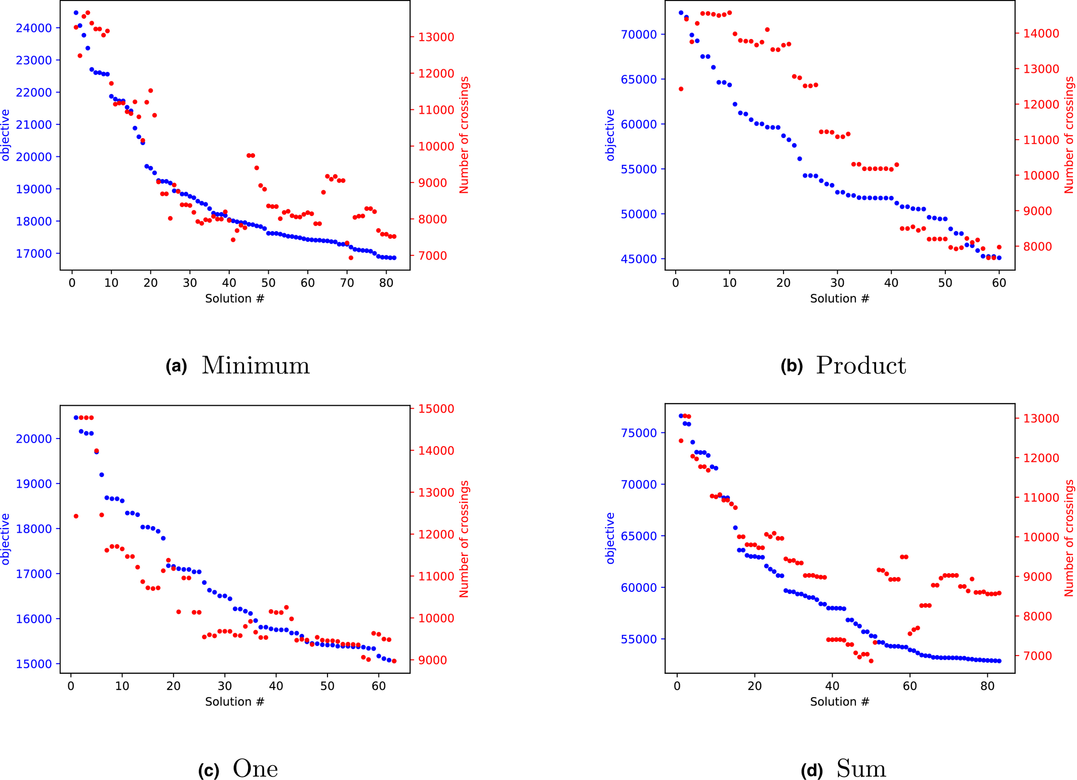
For Each Feasible Point, the Objective Function Value on the Left Axis and the Number of Crossings as Output of the Simulation Model are Shown. Each Graph Corresponds to a Different Objective Function and a Different Run of Algorithm Dynamic Fix‐and‐Relax Pump [Color figure can be viewed at
Each of the four graphs in Figure 6 is generated as follows. For a specific objective function, all computed feasible points by DRFP are sorted according to decreasing objective function value. This is shown by the blue dots. For each feasible point, the resulting crossings, as evaluated by the simulation model, are shown by the red dots. Therefore, in a perfect (that is, dynamic) model, the red dots would lie on the blue line. We observe that the two y‐axis values live on different scales.
Next, we want to evaluate how good the obtained solutions (“blue dots”) mimic the simulation results (“red dots”); therefore, consider Table 5. This table lists both the Pearson correlation and the Spearman's rank correlation of the objective function value to the simulation result. Such as the correlation, the rank correlation lies between −1 and +1 and a value close to +1 indicates strong dependence. While the correlation measures linear dependence, the rank correlation captures monotonic relationships, that is, only the ranks of the data points are compared and not their values. Therefore, the rank correlation is a more relevant measure for our data than the correlation because we are just interested which solutions perform best.
Comparison of Relationship between Objective Function Value and Simulation Result
For the results in Figure 6, the “product” objective function value performs very strong for both the correlation and the rank correlation. The “sum” and “minimum” objectives perform well with respect to the correlation of objective values and simulation results but show weaknesses with respect to rank correlation. That can also be seen in Figure 6 since for both objectives there exist points with very good objective values but poor simulation performance. It is striking to see that also the “one” objective performs very well for both performance measures. However, while the results for “sum,” “minimum,” and “product” have been very similar in previous versions of the numerical results, “one” did behave much worse in these runs. So, the good performance of “one” might be a ”lucky shot” caused by the stochastic nature of DFRP.
Finally, for each objective function, the best feasible points with respect to their objective value and the simulation result are evaluated with the second, much more detailed simulation model. Because for the “one” objective these points coincide, we computed the number of FIFO crossings for seven feasible points and ended up with the results in Table 6.
Computation of Critical FIFO Crossings for the Best Seven Solutions Found by Dynamic Fix‐and‐Relax Pump (DFRP) Evaluated on a Time Period of Three Years
The best solution found without any FIFO crossings is illustrated in Figure 7.
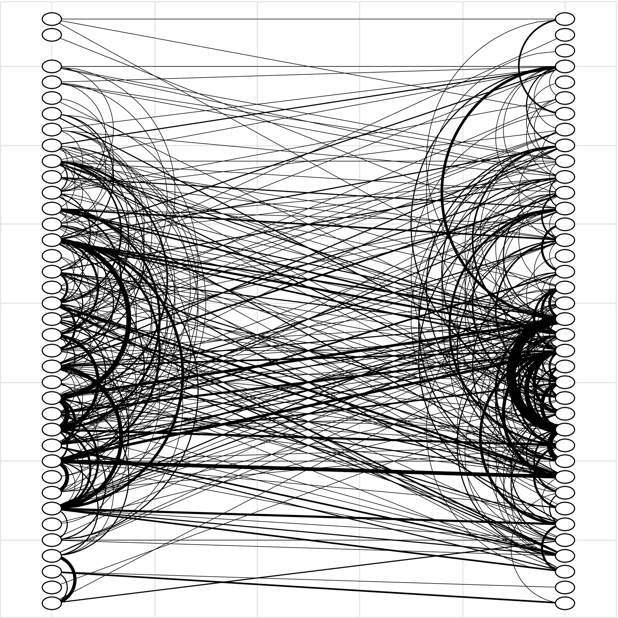
Best Solution with Regard to the Number of Critical FIFO Crossings Computed by Dynamic Fix‐and‐Relax Pump
The final solution was presented to the engineering department. Although we computed a fully feasible layout in the sense that no FIFO crossings occurred on historical connection data, we were aware of the fact that that might not hold true for futures connections. However, the best layout generated by our algorithm reduces the expected number of such events to a few per year, which was deemed to be acceptable by the engineers.
As a side effect, our models provided valuable insights for the engineers. In particular, the question of how many pipes of the different lengths will be needed was an important parameters for the dimensioning of the tube handling system. Also, more general questions, such as the effect of the width of the switching hub (the distance between the two lines of connectors) on other parameters, could be answered easily.
Our results removed the last concerns toward the applicability of the robotic invention, and a decision was made to build it. The robotic system will automatically prevent connections between wrong units, decrease the risk of spillage and increase the safety and satisfaction of the workforce.
Conclusions
In an effort to increase human safety, BASF is developing a dual‐arm robotic system to reconnect pipes in a switching hub. The robot can undertake almost all reconnections, except such reconnections which require the removal of multiple pipes at ones, which is left to the humans. This raised the question on how to design the layout of a new switching hub in order to minimize the number of reconnections involving humans. We have modeled this real‐world problem as a special minimal crossing number problem in conjunction with two simulation models. The resulting edge‐constrained weighted two‐layer crossing number problem (ECW2CN) leads to instances of gigantic size (approximately 70 billion constraints), when tackled via MILP approaches. Therefore, we have developed a tailored Benders decomposition which is employed in a dynamic fix‐and‐relax pump. For different objective functions, we have identified a total of 454 feasible layouts. These layouts are then evaluated by two different simulation models. The obtained solution not only increases human safety but also provides valuable feedback to engineers regarding the design of the switching hub.
We see three possible directions for future academic research. The first direction is to increase the computational efficiency of the tailored solution algorithms or to propose better performing models and methods. For Benders decomposition, there might be possibilities to further strengthen the master problem through tailored cuts. Another possibility might arise when combining column generation (on the τ‐variables) with Benders decomposition. A second direction is to enhance the model by dynamic and stochastic aspects, capturing the entire complexity of the real‐world problem. This comes at the cost that: (1) no real‐world data are available, and (2) the model becomes even more challenging to solve. A third direction is to obtain better theoretic lower bounds through specific crossing number lemmas, taking the special structure of ECW2CN into account.
Footnotes
Acknowledgment
We thank Alfred Krause and his team for the interesting and fruitful collaboration which gave rise to the subject of this article. Furthermore, we thank Debora Morgenstern for handling the project during its first steps. Also, many thanks to Marcel S. Schmidt for assisting with early versions of the numerical computations and creating the visualizations. Finally, we thank Silke Horn, Sonja Mars and Kostja Siefen from GuRoBi for answering our questions about implementation details and Carsten Linz for supporting the project in an outstanding way.