COVID‐19: A multiwave SIR‐based model for learning waves

Abstract

One of the greatest challenges of the COVID‐19 pandemic has been the way evolving regulation, information, and sentiment have driven waves of the disease. Traditional epidemiology models, such as the SIR model, are not equipped to handle these behavioral‐based changes. We propose a novel multiwave susceptible–infected–recovered (SIR) model, which can detect and model the waves of the disease. We bring together the SIR model's compartmental structure with a change‐point detection martingale process to identify new waves. We create a dynamic process where new waves can be flagged and learned in real time. We use this approach to extend the traditional susceptible–exposed–infected–recovered–dead (SEIRD) model into a multiwave SEIRD model and test it on forecasting COVID‐19 cases from the John Hopkins University data set for states in the United States. We find that compared to the traditional SEIRD model, the multiwave SEIRD model improves mean absolute percentage error (MAPE) by 15%–25% for the United States. We benchmark the multiwave SEIRD model against top performing Center for Disease Control (CDC) models for COVID‐19 and find that the multiwave SERID model is able to outperform the majority of CDC models in long‐term predictions.

INTRODUCTION

COVID‐19 is an infectious disease caused by acute respiratory syndrome (SARS‐CoV‐2) (World Health Organization, 2020a). Although the disease was first identified in 2019 in Wuhan, Central China, since then, it has quickly spread globally, resulting in an international health crisis, also often referred to as the 2019–2020 coronavirus pandemic (Hui et al., 2020; World Health Organization, 2020c). A major contributor to the rapid spread of the disease in 2020 was the combination of limited testing resources, an unquantified proportion of asymptomatic cases (World Health Organization, 2020b), and the lack of a vaccine or specific antiviral treatment. On January 21, 2020, the United States identified its first confirmed case of COVID‐19 (Haynes et al., 2020) and since then, the disease has spread rapidly through the country resulting in major economic and social change. This has included but is not limited to, nearly 442,000 dead in just the United States as of February 1, 2021, massive unemployment, reaching as high as

$14.7\%$

in April 2020 (U.S. Bureau of Labor Statistics, 2020), a decrease in gross domestic product (GDP) of

$31.7\%$

for the second quarter of 2020 (U.S. Bureau of Economic Analysis, 2020), and massive societal change as nearly

$42\%$

of U.S. labor shifted to work from home (Stanford Institute for Economic Policy Research, 2020).

A significant driver of this economic and social change has been the lack of widespread pharmaceutical interventions that would slow the spread of the disease. Even as vaccines are being administered across the country, most states have prioritized healthcare professionals, high‐risk civilians, and essential workers. As such, government, companies, and leaders have had to turn to other prevention measures to slow the disease among the larger population. Methods for intervention have included social distancing, work from home mandates, limits on the size of public gatherings, and mask requirements. These interventions proved effective at first, curbing the first wave of COVID‐19 cases in April 2020. However, when many of these measures were rolled back and people grew tired of quarantine practices in late spring and early summer of 2020, cases surged in a second, significantly larger wave. This pattern was repeated again in the fall and winter of 2020, as the return of students to school combined with the many end‐of‐year holidays created a massive spike in cases at the end of the year. This spike continued to drive higher with each successive winter holiday, Thanksgiving, Christmas, and New Year, until January 8, when the wave reached its height (Johns Hopkins University, 2020). This has been particularly challenging because the traditional epidemiology SIR model, upon which most of the modeling efforts have been based, only captures single waves.

For COVID‐19 and for many other epidemics, modeling a single wave will not be able to capture the nature of the disease. The problem is further complicated by the many different possible drivers of waves (e.g., behavioral changes, medical practices, disease evolution). In practice, it will often be impractical to try and capture all the different drivers that could affect changes on the epidemic through data. For example, if it seems like a new wave is starting, is this wave driven by behavior changes, such as people becoming more social? Have people's willingness to comply with mask mandates or social distancing changed? Is it due to changes in temperature or environment that is making the disease more infectious? Is it due to a new variant of the disease emerging? Some of these features can be incorporated in the model (e.g., mobility, temperature) but others are hard to quantify on a timely basis (e.g., new variants, compliance with restrictions). Furthermore, to incorporate all features that could possibly affect the disease will create a model that is first, difficult to learn parameters for, and second, hard to generalize as the model will only be applicable to the epidemic it is built for.

In this paper, we propose a highly generalizable extension on the susceptible–infected–recovered or SIR‐based model (SIR and its many additional compartment extensions, such as the SIRD (susceptible–infected–recovered‐deceased), SEIR (susceptible–exposed‐infected–recovered), and SIRS (susceptible–infected–recovered‐susceptible)), which allows the traditional epidemiology models to accurately identify and capture multiple waves. The model's ability to detect new waves is not dependent on expert advice to know key drivers of infections or data availability of these drivers. We show that in cases where changes in the nature of the epidemic have resulted in multiple waves, our model is able to appropriately identify and characterize these multiple waves. We then describe an algorithm that is able to learn the multiwave SIR model and prove that the algorithm will identify a change in infection rate and characterize how quickly the identification will occur. Finally, we show experimentally how the multiwave model allows for higher predictive accuracy and conclude with how this work can improve operations and supply chain management during a pandemic.

CONTRIBUTIONS

Our main contribution through this work is introducing a multiwave SIR model and establishing guarantees on the rate of learning. Furthermore, we demonstrate significant improvements in forecasting of the COVID‐19 pandemic for the different states in the United States. We summarize our contributions as follows:

We introduce the multiwave SIR‐based models: We develop an SIR‐based model that is able to account for multiple waves regardless of the waves' drivers. The model is driven by the reality of multiple waves in cases experienced by many states across the United States and the world and investigates an area of SIR epidemiological modeling that has been largely underexplored.

We propose an algorithm to learn the model from data: We introduce a dynamic method for learning the waves of an epidemic that requires no priors on the number of waves in the data or the infection/recovery rate of each wave, which would have been hard to know in advance. The algorithm combines traditional probabilistic methods for learning SIR models with a martingale framework for detecting change points in data streams. The proposed algorithm is fast, scalable, and works with live data streams.

We give theoretical guarantees on how fast we can detect new waves: We leverage the martingale framework to create bounds on how fast we expect to detect a new wave of an epidemic. The bound is dependent on the parameters of the model, the population size, and difference in infection rates between subsequent waves. Specifically for the parameters we use when modeling COVID‐19, we show that we expect to flag a new wave within half of a week.

We show strong computational results on COVID‐19 data: We show how the multiwave model is able to create significant improvement in terms of forecasted infection accuracy. We describe how this multiwave SIR model can be adapted into a multiwave SEIRD (susceptible–exposed–infected–recovered–dead) model and outperform the original SEIRD in in‐sample fit and out‐of‐sample accuracy. We demonstrate that this performance is comparable with top COVID‐19 forecasting models used by the Center for Disease Control (CDC). The SEIRD model is used because of its wider popularity. Furthermore, it is more expressive because of larger number of compartments in the model.

LITERATURE REVIEW

Since the onset of COVID‐19 pandemic, there has been a renewed interest in the modeling and analysis of epidemiological models in the operations community. Since in the current paper we consider both predictive and prescriptive problems based on epidemiological models, we briefly discuss relevant studies from both aspects in what follows.

The SIR epidemic model forms the basis of the multiwave modeling used in the current paper. It is a compartmental epidemiological model that was first used by Kermack and McKendrick (1927). Compartmental models consider mathematical modeling of infectious diseases in which the overall population is divided into different compartments, for example, susceptible, infectious, and recovered (SIR). Differential equations are then used to model the transition of the population from one compartment to another. Since its introduction, the SIR compartmental model has been extended and analyzed in various forms. One such extension known as the SEIRD model considers further compartmentalization of the population into two extra compartments of the exposed (E) and the deceased (D) population. Various other extensions have been considered and we refer the interested readers to Brauer (2008) for a detailed discussion.

Compartmental epidemiological models crucially rely on important model parameters such as infection rate and transmission rate. Very few studies focus on the problem of estimating these parameters from data. Cantó et al. (2017) consider the problem of identification and estimation of the SIR model parameters and develop algorithms to estimate model parameters using a least‐squares methodology. Similarly, Marcondes (2020) proposes a robust parameter estimation technique that uses goodness of fit on out‐of‐sample data to estimate the SIR model parameters. Others like Li et al. (2018) use media coverage to augment the SIR model and then show how to estimate different model parameters. More recently Baek et al. (2020) analyze the limits of SIR model parameter estimation and in‐turn prove that no unbiased estimator can provide accurate estimates of the model parameter until observing enough of the pandemic. The current work is complimentary to these studies since it focuses on understanding how to model and detect multiple waves of a pandemic.

The paper is also related to change‐point detection in the context of epidemiological models. Change‐point detection is a widely studied topic in varied fields including statistics, finance, and most recently in operations and demand forecasting. For a brief overview of the various applications and techniques used for change‐point detection, we refer the interested readers to the survey paper by Aminikhanghahi and Cook (2017). Our approach most closely resembles that of probabilistic methods where the central assumption is that the sequence of observations may be divided into nonoverlapping state partitions, and the data from each partition is sampled i.i.d from an underlying distribution (Adams & MacKay, 2007). Veeravalli and Banerjee (2014) consider a general time series process with a change point that needs to be detected and recover mini‐max and Bayesian formulations and guarantees for how fast the wave can be detected. While similar in spirit, the authors' model differs from the model of the current paper in multiple ways. First, they consider a Bayesian framework where the change point itself has a prior distribution. Second, and more importantly, the authors assume that the observations are i.i.d. and the distribution parameters shifts after the change point. Contrasting this to the current paper, the observations in our case are cases (deaths), which are not i.i.d. because of the underlying compartmental model that governs the dynamics of the system. As such the analysis depends on carefully modeling a martingale process from the observed cases (deaths) that is then analyzed using large deviations theory. Since the current paper focuses on an epidemiological application, we discuss the relevant papers in this application domain in more detail. Texier et al. (2016) consider the problem of estimating not just the start, but also the end of a pandemic using change‐point detection methods. Since they still focus on a single wave, our work differs considerably from theirs. More recently, Jiang et al. (2021) focus on detecting multiple waves of a pandemic using a Bayesian Poisson segmented regression model. While our work and theirs both focus on being able to flag change points in the pandemic and then training SIR parameters that only vary at the change point, the method of detection differs greatly. Specifically, Jiang et al. (2021) detect waves all at once, resulting in a process that requires knowledge of subsequent waves in order to characterize and model a specific wave. Our method models waves in a sequential fashion that allows for wave detection in real time. Similarly, Juodakis and Marsland (2020) show how to estimate change points in a pandemic in the presence of noisy observations. The paper uses a log‐likelihood method along with modeling of a background parameter to estimate change points in the epidemic. We set ourselves apart from these works, first by proposing a real‐time method of detecting when a wave is occurring by tracking when the predictive power of the SIR model suddenly deteriorates and proving theoretically we will be able to detect a new wave within approximately half of a week.

There has been a considerable effort from the research community to analyze the disease evolution of the COVID‐19 pandemic. See, for example, Anastassopoulou et al. (2020), Calafiore et al. (2020), Gaeta (2020), Giordano et al. (2020), Kucharski et al. (2020), Li et al. (2020a), Wu et al. (2020), among various others. These studies aim at developing both analytical as well as data‐driven tools to understand the pandemic. Pham et al. (2020) provide a brief overview of machine learning–based studies for prediction. Nevertheless, none of these studies focus on developing analytical tools for analyzing multiple waves of the pandemic, the focus of the current work. Recent works have also focused on modeling multiple waves of the pandemic using compartmental models. Kaxiras and Neofotistos (2020) consider a multiwave SIR model that extends the SIR model proposed by the same authors. The model captures the effect of lockdowns by incorporating a time‐changing parameter in the underlying model that causes the number of infections to go down once a lockdown is imposed. More generally, Flaxman et al. (2020) consider a Bayesian hierarchical model to infer the effect of different interventions on the number of infections over time. Similarly, Tang et al. (2021) also focus on known changes in model parameters related to known interventions that drive changes in the pandemic case counts. Finally, Tat Dat et al. (2020) use wavelet theory and machine learning to directly fit wavelet models to estimate cases. All the aforementioned studies assume that the time of the change in parameters is known and is not learnt from the data. We focus on the case when the parameters of the underlying model shift, but not necessarily due to known interventions. Hence, our estimation problem becomes considerably harder. Furthermore, we also provide analytical guarantees on the learning rate of the change point, providing analytical justification to the modeling framework.

Researchers have also focused on empirically quantifying the effect of different interventions on the spread of the pandemic. For example, Fang et al. (2020) quantify the impact of mobility restriction in Wuhan on the containment and delay in the spread of the virus, Friedson et al. (2020) focus on the effect of the shelter in place order in California, and Chiou and Tucker (2020) discuss the role of diffusion on an individual's ability to self‐isolate and find that income and Internet access are correlated with an individual's ability to self‐isolate. Similarly, Allcott et al. (2020) provide evidence on the drivers of the early U.S. pandemic using a compartmental model and find that the main drivers are population density and static characteristics of the state. Others, such as Flaxman et al. (2020) consider a renewal process to model the number of infected individuals and consider six different levels of intervention, which directly impact the reproduction number in the SIR models. While the studies cited above focus on measuring the effect of specific interventions on the spread of the pandemic, the current work focuses on the estimation of general shifts that are agnostic to what could be driving that change, regardless of whether it is changes in government intervention, mobility, or new variant.

Finally, there has also been a considerable upsurge in operations management related prescriptive studies related to the COVID‐19 pandemic. For example, Chen et al. (2020) focus on optimal allocation of vaccines with limited supply. In contrast, Birge et al. (2020) focus on developing optimal targeted lockdown policies to control the spread of disease in a population. Bertsimas et al. (2021) create a decision support tool for both governments and individuals to aid in various decision‐making problems during the pandemic. Finally, Agca et al. (2020) study the impact of COVID‐19 on supply chain credit risk. Similarly, Cao et al. (2020) study the impact of the pandemic of gig economy and find substantial differential impact of the pandemic across different groups. Furthermore, Li et al. (2020b) focus on finding the impact of government interventions on the spread of the pandemic.

A MULTIWAVE SIR‐BASED MODEL

Intuition and model preliminaries

We first describe the original SIR model upon which we are building the proposed multiwave model. We then describe the two‐wave SIR model and finally, discuss the multiwave SIR model. Compartmental epidemiology models, such as the original SIR model, are based on the idea that a given population experiencing an epidemic can be grouped into subgroups or compartments that can be then used to characterize the spread of the disease. The original SIR model (Kermack & McKendrick, 1927) has three such compartments: susceptible, infected, and recovered. People move from being susceptible (S) to the epidemic, to becoming infected (I) and finally recovering (R), hence the name SIR. The order of the letters in the name often indicates the flow of the population through the compartments. Because the entire population is split into these compartments the size of the total population can be found by summing the size of each individual compartment. The SIR is considered the simplest of the compartmental epidemiology models, but most of the extensions are based on this foundation. A few examples of popular extensions include accounting for populations that deceased rather than recovered (SIRD), instances where people lose immunity and move from recovered to susceptible again (SIRS) and a compartment for people exposed to the disease but not yet infectious (SEIR). Movement between compartments in the SIR model is determined by the size of each compartment and two parameters, the infection rate

$\beta$

and recovery rate

$\gamma$

. The SIR model is governed by three equations, where at time

$t$

,

$S_t$

is the size of the susceptible population,

$I_t$

is the size of the infected population,

$R_t$

is the size of the recovered population, and

$N$

is the total population (

$N=S_t+I_t+R_t$

):

1

By the nature of these equations, the original SIR model assumes that once the infected population has started to decline, it will not increase again.

$N$

,

$\beta$

, and

$\gamma$

are constants and because the differential of the susceptible population is nonpositive the susceptible population will never get bigger. Therefore, if the infected population has started to decline, indicating that

$\frac{\beta \mathrm{SI}}{N}-\gamma I<0$

, then as the size of the susceptible population continues to fall,

$\frac{\beta S}{N}$

will only continue to get smaller ensuring that the differential of the infected population remains negative. This suggests that the traditional SIR model will always predict that once a single wave has occurred, the disease will die out. Unfortunately, a single wave has not been the case in most regions around the United States and in many other countries.

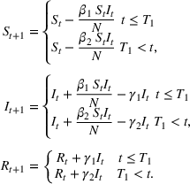
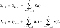
In the two‐wave SIR model, we start with the original SIR model. However, in this new model, there is a time

$T_1$

, when wave 1 ends and wave 2 starts, where the infection and recovery rates change from

${\beta }_1$

and

${\gamma }_1$

to

${\beta }_2$

and

${\gamma }_2$

. As we discuss in Section 3, our algorithm learns when this time

$T_1$

occurs. The number of individuals in each compartment remains the same, but at time

$T_1+1$

the system is characterized by new parameters,

${\beta }_2$

and

${\gamma }_2$

. Thus the two‐wave model can be characterized by the following three equations:

2

Intuitively,

$T_1$

can be thought of as the time of the onset of the second wave. At time

$T_1$

, some behavior about the population has changed resulting in a different rate of infection or recovery and we recalibrate the model accordingly. For example, in states where government restrictions were lifted resulting in a second wave,

${\beta }_1$

would represent the infection rate when government measures were in place,

$T_1$

would correspond with the lifting of restriction, and

${\beta }_2$

would be the unconstrained rate of disease spread.

While we showed previously that the original SIR model is unable to model multiple waves, this model will be flexible enough to capture two waves. If time

$T_1$

falls after the first peak, then even when

$\frac{{\beta }_1\mathrm{SI}}{N}-{\gamma }_{1}I<0$

as it would be after the first peak, as long as neither the susceptible nor infected populations are zero, either

${\beta }_2$

or

${\gamma }_2$

can make the differential positive again. In this case, the model will predict two waves for the infection.

When we consider a single change point

$T_1$

then the model will consider, at most, two waves. However, we can extend the model to multiple waves by considering multiple change points. If we wish to model

$\overline{n}$

waves, we can consider change points,

$T_1,T_2,\cdots ,T_{\overline{n}-1}$

, and corresponding parameters

${\beta }_1,{\gamma }_1,{\beta }_2,{\gamma }_2,\cdots ,{\beta }_{\overline{n}},{\gamma }_{\overline{n}}$

. We will discuss in Section 4.3 how to determine the number of waves dynamically as the disease evolves.

There are two parts to learning the parameters of the multiwave SIR model. One, we need to detect the change points,

$T_1,T_2,\cdots$

in order to segment the epidemic into waves. Two, for each wave, we need to learn the parameters for the SIR model. We propose a dynamic approach to learning both the change points and the infection/recovery rates. We assume in our training data we have for daily information on,

$i(t)$

, the number of new cases, and

$r(t)$

, the number of recovered cases on each day

$t$

. Given these data, we calculate the starting condition of the wave, either from the initial conditions of the epidemic or the end conditions of the previously modeled wave. Using the initial conditions and the data up to day

$t$

, we learn the “best” parameters for the wave happening. Then, based on these parameters, we evaluate whether a change point has occurred, indicating a new wave has started. If a new wave has not happened, then we move on to the next day, updating our assessment of the parameters. If a new wave has started we record the population compartments on day

$t$

as the initial conditions of the new wave.

SIR parameters

For a given wave

$n$

, the parameters are only dependent on the initial conditions of the wave (number of susceptible, infected, and recovered at the start of the wave) and data recorded during the wave. We do not need to know any information about the subsequent waves to learn these parameters. At the start of an epidemic, we can learn the first wave parameters directly from the data on new infection/recoveries. For each wave thereafter, training occurs sequentially. We use the learned parameters to help detect new waves and if a new wave is flagged, we then use end conditions of the wave we are in as the initial conditions of the new wave so that we can learn the new wave's parameters.

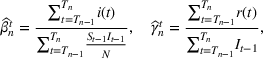
For the single‐wave model, it has been shown that learning the infection rate and recovery rate can occur quickly. The number of new infections/recovered can be modeled as a Poisson distribution and can be solved for directly using initial conditions and data (Li et al., 2018). Consider wave

$n$

that starts at time

$T_{n-1}$

and ends at time

$T_n$

and assume the

$n-1$

previous waves have been modeled. Then we would have already modeled the initial conditions,

$S_{T_{n-1}}$

and

$I_{T_{n-1}}$

and previous literature (Li et al., 2018, Hong & Li, 2020) show that we can estimate the paramters of wave

$n$

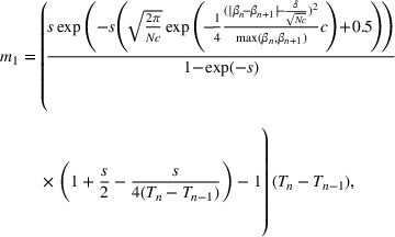
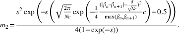
as:

$$\begin{array}{c}\hfill {\widehat{\beta }}_n^t=\frac{{\sum }_{t=T_{n-1}}^{T_n}i(t)}{{\sum }_{t=T_{n-1}}^{T_n}\frac{S_{t-1}{I}_{t-1}}{N}},{\widehat{\gamma }}_n^t=\frac{{\sum }_{t=T_{n-1}}^{T_n}r(t)}{{\sum }_{t=T_{n-1}}^{T_n}{I}_{t-1}},\end{array}$$

3

where

4

Nevertheless, the estimation process does not always produce the most accurate results in practice, so the estimates for

${\widehat{\beta }}_n^t$

and

${\widehat{\gamma }}_n^t$

need to be further optimized. As a result, we use the above as a warm start in a maximum likelihood estimation procedure. Note that we do not need any information on future waves to estimate the parameters of the current wave.

Change points

Before discussing change points, it is worth first explicitly defining what a “wave” is. For the sake of our model, we will define a wave as a section of time when the dynamics of the epidemic are relatively stable such that constant parameters in the SIR model are able to describe the spread of the disease. This means that the errors of a well‐tuned SIR model should just be noise, without a trend to them. A new wave is said to have happened when the dynamics of the underlying epidemic have changed such that the trained parameters are no longer able to describe the epidemic. The key to wave detection then becomes identifying when the errors of the model are no longer just noise but rather represent a shift in the underlying infection rate. To accomplish this, we apply a martingale framework in time‐varying data streams (Ho, 2005) to the infection/recovery rate of the SIR model. In particular, the approach follows three key steps:

• 1.

First, we define an error score per time period (

$Z_t$

) based on weighted error in predictions to estimate how strange or unusual a data point is.

2.

Using these error scores over a time scale, we define a p‐value (

$p_t$

) that undergoes a distributional shift, whenever there is a change point in the underlying time series.

3.

Finally, using the p‐values, we define a martingale sequence and use a threshold test to check if the martingale has shifted away significantly. This threshold test is used to flag a new wave in the time series.

We note that while similar in spirit, the approach differs considerably from existing change‐point detection methods. Whereas most change‐point papers assume access to a stream of observations that are sampled i.i.d (see, e.g., Adams & MacKay, 2007; Harchaoui et al., 2009; Haynes et al., 2017; Veeravalli & Banerjee, 2014), the observations in the current paper are COVID‐19 cases (deaths) that are not i.i.d. because of the underlying compartmental model that governs the dynamics of the system. As such the analysis depends on carefully modeling a martingale process from the observed cases (deaths) that is then analyzed using large deviations theory.

Error scores

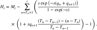
First, we consider how the model looks when a new wave has not started. Let us assume again that waves

$1\cdots n-1$

have been modeled, and we are considering wave

$n$

, which begins on day

$T_{n-1}$

and ends on day

$T_n$

. On each day

$t\in [T_{n-1},T_n]$

, we calculate our best estimate of wave

$n$

's infection rate,

${\widehat{\beta }}_n^t$

and predict our estimate of the number of new infections,

$\widehat{i_t}=\frac{{\widehat{\beta }}_n^t{S}_t{I}_t}{N}$

. We can use the weighted error on this prediction,

$Z_t=\frac{|\widehat{i_t}-i_t|}{\sqrt{S_t{I}_t}}$

, to understand how strange or unusual a new data point is. During the same wave, these errors should be identically distributed. Intuitively, this is because as long as we have a good estimate of the infection rate, the data points are all part of the same wave and after we weight to account for changing susceptible/infection levels, we have no prior on any days being more or less prone to error. We make the following technical assumption on the estimation error of the individual wave parameters, to quantify the effect of estimation error on time to detect waves. Assumption 1

Let

${\widehat{\beta }}_n^t$

denote the estimate of the infection rate of the underlying wave

$n$

at time step t. Then,

$\exists \delta \ge 0$

such that

$$|{\widehat{\beta }}_n^t-{\beta }_n|=\frac{\delta }{\sqrt{S_t{I}_t}},$$

5

where

$S_t$

and

$I_t$

denote the susceptible and infected population at time t.

The assumption above ensures that the error in the estimation of the wave parameters is bounded as a function of the compartmental model parameters,

$S_t$

and

$I_t$

.

$\delta$

is the estimation error parameter that is large when the estimation of the underlying infection rate is not accurate and small otherwise. Note that we only assume the existence of such

$\delta$

but not its knowledge for the proposed change‐point detection method to work.

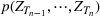
We show next that the error scores constructed above follow an important property: They are exchangeable within a wave. That is, they are i.i.d. Note that the same does not hold for the observed sequence of cases (deaths). Proposition 1

The weighted sequence of errors within the same wave,

$$\left\{Z_t=\frac{|\widehat{i_t}-i_t|}{\sqrt{S_t{I}_t}}:T_{n-1}\le t\le T_n\right\}$$

6

$\forall n$

is exchangeable, that is, the joint distribution

$p(Z_{T_{n-1}},\cdots ,Z_{T_n})$

does not change under any permutation of the indexes.

Proof 1

See Supporting Information Appendix S1.

$\square$

We call this sequence of errors the strangeness scores of the data points.

Exchangeability of the strangeness scores no longer holds true when a new wave has begun. Let us consider the days

$T_{n-1}$

to

$T_{n+1}$

where a new wave begins at time

$T_n$

. Then the error between

$T_{n-1}$

and

$T_n$

will be exchangeable, but this will not be true after

$T_n$

. We expect the error to go up because the infection rate has changed and we will be using the infection rate from wave

$n$

to model what is happening in wave

$n+1$

. Thus, we can test whether a new wave has started by checking exchangeability, which consists largely of two steps (Vovk et al., 2003). First, we calculate a p‐value measuring the proportion of previous instances that had errors equal to or bigger than the current data point.

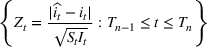
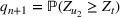
Calculating p‐values and defining a martingale sequence

Let

$p_t$

be defined as the following:

$$p_t=\frac{{\sum }_{u=T_{n-1}}^t{\mathbb{1}}_{Z_u\ge Z_t}}{t-T_{n-1}}.$$

7

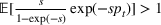
As long as the underlying error remains exchangeable, then

$p_t$

is distributed uniformly in [0,1] (Vovk et al., 2003). However, when the next wave hits, we expect

$p_t$

to drop closer to 0 for a while, on account of larger estimation error.

The key then becomes determining when

$p_t$

is no longer uniformly distributed. We do this by creating a martingale

$M_t$

, using a sensitivity parameter

$s$

$$M_t=\prod _{u=T_{n-1}}^t\frac{s}{1-\exp (-s)}\exp (-s{p}_u),$$

8

where the martingale is initialized at some value,

$M_0$

. It is worth noting that

$M_t=M_{t-1}\frac{s}{1-\exp (-s)}\exp (-s{p}_t)$

. First, this shows that it is not necessary to store the entire history of

$p_t$

. Second, it helps demonstrate that as long as

$p_t$

is uniformly distributed,

$M_t$

is a martingale because,

$$\begin{array}{c}\hfill \mathbb{E}[M_t|M_{t-1}]=M_{t-1}\mathbb{E}\left[\frac{s}{1-\exp (-s)}\exp (-s{p}_t)\right]=M_{t-1}.\end{array}$$

9

As long as

$p_t$

is uniformly distributed, we expect

$M_t$

to remain around

$M_0$

. However, when

$p_t$

drops,

$M_t$

will rapidly grow signaling a wave has occurred. In general, the only selection requirement for

$s$

is that it must be positive, but the larger

$s$

is, the more sensitive

$M_t$

is to changes in infection rate. In our experiments we have found

$s=2.1$

is a reasonable value for this parameter allowing the model to be sensitive to wave changes without overflagging.

We use a threshold test in order to determine when

$M_t$

has deviated significantly far away from

$M_0$

(Ho, 2005; Vovk et al., 2003). Note that to ensure that the martingale is not too sensitive with respect to initial estimates of the parameters, whenever

$M_t$

drops below 1, we reset the strangeness scores and martingale. We set a threshold,

$\lambda >M_0$

, and next define the concept of

$\lambda$

‐detectable waves. Definition 1

$\mathit{\lambda }$

‐Detectable Waves

Let

$M_t$

be the martingale sequence defined as before. Then, a wave is

$\lambda$

‐detectable if there exists some time

$t$

within the length of the wave, such that

$M_t>\lambda$

.

Notice that if

$M_t>\lambda$

, then we have detected a new wave and we reset the martingale and strangeness scores, and begin learning the parameters of the new wave. The challenge is to determine values for

$\lambda$

that are large enough that we are not overly sensitive to white noise but small enough so that we can quickly identify new waves, without missing anything. In the following sections, we will characterize the expected time that it takes for this approach of using martingales to identify new waves based on the relationship between

$s$

,

$\lambda$

,

$M_0$

, and the other attributes of the epidemic.

FINITE SAMPLE GUARANTEES: HOW FAST DO WE DETECT A NEW WAVE?

In this section, we discuss the expected time it takes to flag a

$\lambda$

‐detectable wave in the model. We start by first demonstrating that when a new wave hits, the martingale,

$M_t$

, becomes a submartingale and characterize the rate of growth of the submartingale. We then use the growth rate along with optional stopping theorem to prove bounds on the expected detection time. For the rest of this section, we will focus on the case when a new wave results in increasing daily new cases. This assumption is only made for analytical tractability and we note that the multiwave model works for all new waves. Furthermore, it is in this situation when the number of cases are going up that rapid wave detection is most relevant.

Let us say that wave

$n+1$

has just kicked off but the model has not flagged it yet. This means that the martingale would be still considering all the data from wave

$n$

, which went from time

$T_{n-1}$

to

$T_n$

, along with all the data from the new wave.

When the

$n+1$

wave hits at

$T_n$

,

$M_t$

becomes a submartingale. This is because when a new wave occurs,

$p_t$

is no longer uniform. The model will still be making predictions based on wave

$n$

, but the new infections will be driven by the parameters of wave

$n+1$

. This will result in higher strangeness scores,

$Z_t$

, which are the weighted difference between the predicted and actual new infections, causing

$p_t$

to skew closer to 0. When this happens,

$\mathbb{E}[\frac{s}{1-\exp (-s)}\exp (-s{p}_t)]>1$

, causing

$M_t$

to become a submartingale.

$M_t$

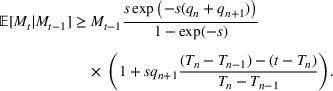
will be expected to grow until it hits

$\lambda$

, flagging a new wave. Theorem 1 introduces a lower bound on the growth rate of the submartingale, which we use to estimate how long it will take

$M_t$

to hit the threshold. Theorem 1

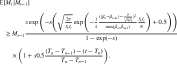
Consider a

$\lambda$

‐detectable wave that starts at

$T_n$

, and assume submartingale,

$M_t<\lambda$

for

$t>T_n$

, so that a wave

$n+1$

has occurred but a new wave has not been flagged yet. Let

$s$

be the martingale's sensitivity parameter,

${\beta }_n$

represent the infection parameter of wave

$n$

, and

$S_t$

,

$I_t$

, and

$N$

be the susceptible, infected, and total populations, respectively. Then the submartingale's expected growth on day t can be bounded as:

10

Proof 2

See Supporting Information Appendix S1.

$\square$

Theorem 1 shows that the growth rate is largest for days right after a change point has happened. It is here, when

$t$

is small and the martingale is growing the fastest, that we are most likely to detect the new wave. The farther

$t$

gets, the smaller the growth rate of the martingale becomes.

Given that the wave is just starting, Theorem 1 shows us that beyond the model parameters, the speed at which

$M_t$

grows is largely dependent on (1) the proportional difference between the infection rates of wave

$n$

and

$n+1$

, and (2) the size of susceptible/infected populations. This makes sense intuitively. We would expect that if the infection rates between waves change dramatically, the model should quickly identify a new wave has occurred. Furthermore, if there is a large susceptible/infected population relative to the total population, changes in infection rate will be amplified making new waves easier to flag.

To prove Theorem 1 we first use the martingale formulation to analyze the structure of the growth rate of the martingale in terms of other problem parameters in Proposition 2. Then we characterize the relationship of the strangeness scores in the new wave (Lemma 1) and between the new wave and old wave (Lemma 2) to prove Theorem 1.

First, we recall that if we let

$t$

be sometime after the wave

$n+1$

has started and recall that

$Z_u=\frac{|\widehat{i_u}-i_u|}{\sqrt{S_u{I}_u}}$

. Let

$u_1$

be a time in wave

$n$

, then the

$\mathbb{P}(Z_{u_1}>Z_t)$

is the probability that the weighted error in the wave

$n$

is greater than the weighted error in wave

$n+1$

. Similarly, if

$u_2$

is a time in wave

$n+1$

such that

$u_2<t$

,

$\mathbb{P}(Z_{u_2}>Z_t)$

is the probability that the weighted error earlier in wave

$n+1$

is greater than the weighted error later in the wave at time

$t$

. Proposition 2

Let

$t$

be a day in wave

$n+1$

so that

$t>T_n$

. Let

$q_n$

represent the probability that the strangeness score,

$Z$

, on a day in wave

$n$

is higher than the strangeness score on day

$t$

and let

$q_{n+1}$

be the probability that the strangeness score on a day before

$t$

in wave

$n+1$

is higher than the strangeness score on day

$t$

, we have:

11

Proof 3

See Supporting Information Appendix S1.

$\square$

Notice that to analyze the growth rate of the martingale, we now need to upper bound probabilities

$q_n$

and

$q_{n+1}$

. We focus on upper bounding these two quantities next. We start by stating Lemma 1 that upper bounds

$q_{n+1}$

. Lemma 1

Let

$q_{n+1}=\mathbb{P}(Z_{u_2}\ge Z_t)$

, for

$T_n<u_2<t$

or the probability that the strangeness score on a day before

$t$

in wave

$n+1$

is higher than the strangeness score on day

$t$

. Then

$q_{n+1}\le 0.5$

Proof 4

See Supporting Information Appendix S1.

$\square$

Lemma 1 provides a coarse upper bound on

$q_{n+1}$

. In Lemma 2 we provide a stronger bound on

$q_n$

by leveraging the fact that the errors will increase when the new wave hits because we will be using an infection rate from wave

$n$

to predict for wave

$n+1$

. Lemma 2

Let

$q_n=\mathbb{P}(Z_{u_1}\ge Z_t)$

, for

$u_1\in [T_{n-1},T_n]$

and

$t>T_n$

or the probability that the strangeness score on a day in wave

$n$

is higher than the strangeness score on day

$t$

, which is in wave

$n+1$

. Then

$$q_n\le \sqrt{\frac{2\pi }{S_t{I}_t}}\exp \left(-\frac{1}{4}\frac{(|{\beta }_n-{\beta }_{n+1}{|-\frac{\delta }{\sqrt{S_t{I}_t}})}^2}{\max ({\beta }_n,{\beta }_{n+1})}\frac{S_t{I}_t}{N}\right).$$

12

Proof 5

See Supporting Information Appendix S1.

$\square$

The proof of Lemma 2 follows by integrating over all possible weighted error scores in predicting cases on day

$t$

and using Chernoff bound to upper bound the probability estimates.

Notice that the upper bound on

$q_n$

in Lemma 2, and by extension the lower bound on the martinagale growth rate, grows with both the proportional difference in infection rate between the waves and the size of the population. It is worth noting, as demonstrated by this bound, that it will be hard to identify changes in infection rate when either the susceptible population,

$S_t$

, is low, meaning everyone has either had COVID‐19 or been vaccinated, or when the infected population,

$I_t$

, is low, which usually happens when an epidemic is just starting or about to end.

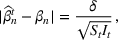
In Theorem 2, we use this growth rate from Theorem 1 to create an upper bound on the expected time it will take the submartingale to hit the threshold. Theorem 2

For any wave

$n$

, let c be a constant such that

$\frac{S_t{I}_t}{N}\ge c>0$

for all

$T_n\le t\le T_{n+1}$

. Then, if the length of the wave is such that,

$$\begin{array}{c}\hfill T_n-T_{n-1}>\frac{\lambda -M_0+\frac{s^2\exp \left(-s\left(\sqrt{\frac{2\pi }{Nc}}\exp \left(-\frac{1}{4}\frac{(|{\beta }_n-{\beta }_{n+1}{|-\frac{\delta }{\sqrt{Nc}})}^2}{\max ({\beta }_n,{\beta }_{n+1})}c\right)+0.5\right)\right)}{4(1-\exp (-s))}}{\frac{s\exp \left(-s\left(\sqrt{\frac{2\pi }{Nc}}\exp \left(-\frac{1}{4}\frac{(|{\beta }_n-{\beta }_{n+1}{|-\frac{\delta }{\sqrt{Nc}})}^2}{\max ({\beta }_n,{\beta }_{n+1})}c\right)+0.5\right)\right)}{1-\exp (-s)}\left(1+\frac{s}{4}\right)-1}\end{array}$$

13

then we can define

$T$

as the time the model successfully detects the new wave and we have that

$$\begin{array}{c}\hfill \mathbb{E}[T-T_n]\le \frac{m_1-\sqrt{m_1^2-4m_2(T_n-T_{n-1})(\lambda -M_0)}}{2m_2},\end{array}$$

14

where

15

$$m_2=\frac{s^2\exp \left(-s\left(\sqrt{\frac{2\pi }{Nc}}\exp \left(-\frac{1}{4}\frac{(|{\beta }_n-{\beta }_{n+1}{|-\frac{\delta }{\sqrt{Nc}})}^2}{\max ({\beta }_n,{\beta }_{n+1})}c\right)+0.5\right)\right)}{4(1-\exp (-s))}.$$

16

Proof 6

See Supporting Information Appendix S1.

$\square$

Theorem 2 provides an upper bound on our expected time to flag a new wave. As we would expect, the upper bound is first driven by the submartingale's sensitivity parameter and the threshold at which we flag a new wave. Second, as with the growth rate, the time till wave detection is driven by the length of waves, the proportional difference in infection rates, and the size of the population. As all of these get bigger, the sooner the model expects to detect a new wave.

To prove Theorem 2, we first create a new variable

$H_t$

based on

$M_t$

, which we show to be a submartingale, and use optional stopping theorem on

$H_t$

to find the upper bound on the expected time till detection. We will not be able to solve for the expected time till detection directly, but we can use an iterative method to solve for tighter and tighter bounds on the time till detection until we get Theorem 2.

Let us define a new submartingale (see Lemma S1 in Supporting Information for a formal proof) for

$t\ge T_n$

, where, as before,

$q_n$

represent the probability that the strangeness score,

$Z$

, on a day in wave

$n$

is higher than the strangeness score on day

$t$

and

$q_{n+1}$

is the probability that the strangeness score on a day before

$t$

in wave

$n+1$

is higher than the strangeness score on day

$t$

:

17

Let

$T$

be the stopping time, the first time that

$M_t\ge \lambda$

, or the time when the new wave is flagged by the model and our estimate of

$T_n$

. We recall that by definition, a wave is

$\lambda$

‐detectable if

$M_t$

hits

$\lambda$

within the length of a wave (where the length of the

$n$

th wave is

$T_{n+1}-T_n$

). Therefore, we have that

$T-T_n\le T_n-T_{n-1}$

. From this we can say that

$\mathbb{E}[T-T_n]\le m(T_n-T_{n-1})$

where

$m\in [0,1]$

. Then the bound is finding the smallest value for

$m$

, which can hold.

We do this by considering optional stopping theorem, given that

$H_t$

is a submartingale. We next check to see if

$T$

, the time we flag a new wave, and

$H_t$

satisfy the requirements of optional stopping theorem, namely, that

$T$

is finite almost surely and

$H_{\min (t,T)}$

is bounded (Williams, 1991). We start by showing that T is finite almost surely. Lemma 3

For all

$t\ge 0$

, there exists some

$T_{\lambda }$

and

$\epsilon >0$

such that:

$\mathbb{P}(T\le t+T_{\lambda })\ge \epsilon$

.

Proof 7

See Supporting Information Appendix S1.

$\square$

Given Lemma 3, we have that

$\mathbb{P}(T<\infty )=1$

(Williams, 1991). Next we check if

$H_{\min (t,T)}$

is bounded, such that there exists a

$b$

such that

$|H_{\min (t,T)}|\le b$

. This is straightforward to check because

$|H_{\min (t,T)}|\le |M_{\min (t,T)}|\le \lambda$

. So we can set

$b=\lambda$

and we satisfy the second requirement of optional stopping theorem. Applying optional stopping theorem allows us to prove Theorem 2.

For our modeling purposes, we have been using

$s=2.1,M_0=203,\lambda =205$

. Given that

$q_{n+1}=0.5$

and when the population is large enough, as is almost always the case when modeling state or county‐level COVID‐19 populations,

$q_n$

becomes negligible. As long as the length of wave (i.e.,

$T_n-T_{n-1}$

) is greater than 8 days, then we have that iterative process for

$m$

holds. Practically for COVID‐19 modeling, this is rarely an issue. However, when the model is applied to epidemics with quick, short waves, users need to be certain to set the threshold

$\lambda$

close enough to

$M_0$

that this is not an issue.

In Table 1 we characterize what the bound looks like in terms of wave length. Choosing the parametric values described in Table 1, we find that the expected time to detect a new wave is half a week or less.

TABLE 1

Upper bound on expected time till detection, given that

$s=2.1,M_0=203,\lambda =205$

and c is significantly large

	$\mathbb{E}[T-T_n]$ bound
Wave length	Upper bound on the expected time to detect a new wave in days
10	4.04
15	3.40
20	3.20
25	3.10

Other epidemiological models

In this work we relax the assumption that parameters of the compartmental epidemiology model are constant, however we inherit the remaining assumptions of the SIR model. For most of these assumptions there are known ways of relaxing them, largely by increasing the number of compartments in the model. The multiwave variation is easily extendable to these variations of compartmental modeling, for example, the computational section of the paper uses an SEIRD model. The analytical results can also be extended easily. In particular, we argue that under the SEIRD model, the only thing that changes in the proof is the way we define the weighted error of the model. We define

$Z_t=\frac{|{\widehat{e}}_t-e_t|}{\sqrt{S_t{I}_t}}$

instead of

$Z_t=\frac{|{\widehat{i}}_t-i_t|}{\sqrt{S_t{I}_t}}$

, where

$e_t$

is the number of new people in the exposed state, and

${\widehat{e}}_t$

the estimated number of new people in the exposed state. The recovered (R) and dead (D) states do not affect the results at all, as what happens to people after leaving the (I) state is irrelevant in the martingale. The rest of the proof and the subsequent results remain unchanged. It is worth noting that the time till detection and ease of learning will vary with the number of compartments. Below we list the main assumptions imposed by the traditional SIR model, how they can be relaxed and accounted for in multiwave model:

• All members of the population are equally susceptible: Due to different demographic effects on the likelihood of contracting COVID‐19, plus differences in behaviors that can reduce an individual's risk (social distancing, quarantining, mask‐wearing, etc.), not everyone is equally susceptible. This is less of an issue when modeling at state level because differences in individual behavior can be averaged across the population. This creates a relatively close approximation for high‐level predictions. However, if this method were to be applied to smaller populations or where differences are more stark, differences in susceptibility can be accounted for by splitting the susceptible population further into subgroups based on their levels of susceptibility.

• All members of the population have equal rates of recovery: Similar to the discussion above we have seen this does not hold true across demographics but can be accounted for by including multiple infected compartments that differentiate different rates of recovery.

• Complete immunity is inferred by recovering from the disease: There has been evidence that this does not hold, as there have been reported cases of people contracting COVID‐19 multiple times, especially as new variants of the disease crop up. The SIRS model is designed to account for this by allowing the recovered population to move back to susceptible at some rate. As long as this recovery rate can be learned or modeled, such that the size of the susceptible population is still known, this does not affect the analytical results we present in this paper.

• The population is closed (no births, deaths—other than that caused by the disease—or migration): Almost all regional populations are not closed. Even in cases where a country is able to lock borders, births and deaths will change the population. When working with state populations, this is less of an issue because the scale of births/deaths/migration is very small compared to the state population. For example, births would only increase the susceptible population by approximately 1.1% and deaths would decrease the population by 0.8% in the United States, thus not really affecting the COVID‐19 forecasts. However, for small populations where births, deaths, or migrations make a difference, rates of incoming and outgoing populations can be accounted for. As long as the model is able to track these changes and can calculate the number of susceptible/infected people, then it will not affect the multiwave model.

• All infections/recoveries are detectable: The SIR model assumes that all movement between compartments (from Susceptible to Infected or from Infected to Recovered) is detectable. This means that there are no asymptomatic cases or testing gaps. Modeling with the SIR when data are incomplete is one of the major challenges of the COVID‐19 pandemic. Asymptomatic cases and insufficient testing can be accounted for by adding an asymptomatic compartment and modeling assumptions around the proportion of asymptomatic cases. It would be difficult to detect waves affecting only the asymptomatic carriers, but the martingale wave detection approach can be applied to the symptomatic cases in the same manner as described in the SIR model.

RESULTS FROM THE DATA

In this section we describe our forecasting efforts using the multiwave SEIRD model for different states in the United States. Specifically, we discuss the data collected, the prediction process, and finally the model's performance in comparison with the original SEIRD model. We note that the SEIRD model is used because of its wider popularity. Furthermore, it is more expressive because of larger number of compartments in the model.

We used data from the John Hopkins Coronavirus Resource Center (Johns Hopkins University, 2020) on daily COVID‐19 cumulative cases and deaths. The JHU COVID‐19 data set is one of the primary sources for COVID‐19 case data in the United States but it does not provide reliable information on active or recovered populations. From the JHU cumulative data, we created active cases feature using a 14‐day rolling sum of the cumulative cases (i.e., active COVID‐19 cases were people who tested positive within the past 14 days) and recovered cases feature by assuming that everyone who tested positive for COVID‐19 but is not an active case or deceased, has recovered. Specifically, we show two sets of results for this paper. The first set is on models trained on state‐level data between April 12, 2020, and September 1, 2020, and then compared out‐of‐sample results on September 2, 2020, through October 1, 2020. The second set is similar, state‐level models but trained up to January 15, 2021, and evaluated out‐of‐sample on results between January 16, 2021, and February 15, 2021.

Given a region, either state or county, and its active, deceased, and recovered populations we trained an SEIRD model and multiwave SEIRD model. We chose to implement an SEIRD model rather than SIR for two reasons. First, because the incubation period for COVID‐19 plays a significant role in its spread, it was important to include an “exposed” population. Second, unfortunately part of COVID‐19's severity is its fatality rate and COIVD‐19 deaths are closely tracked. However, this meant we could use the reliability of the deceased population data to train the model more accurately. In practice, the multiwave SEIRD model is very similar to the multiwave SIR model. Waves are detected in the exact same way, however when training populations and parameters in the wave we use an SEIRD model rather than SIR.

For our results, we use the original SEIRD model as a benchmark for our multiwave SEIRD. The SEIRD model is the most commonly used model for understanding and predicting new cases of COVID‐19. The original SEIRD model is equivalent to a single‐wave multiwave SEIRD model. This means that in states where we do not detect multiple waves, the two models will be exactly the same. However, in cases where multiple waves have occurred, the SEIRD provides a comparison for if the multiwave SEIRD is able to better fit the data.

We describe the out‐of‐sample prediction performance of the SEIRD and multiwave SEIRD models using mean absolute percentage error (MAPE). MAPE is a measure of prediction error such that the lower the value, the more accurate the model. It can be calculated as:

$$\mathrm{MAPE}=\frac{1}{P}\sum _{t=1}^P\frac{|A_t-P_t|}{A_t},$$

18

where here

$P$

is the number of data points being evaluated,

$A_t$

is the actual value of the data point

$t$

, and

$P_t$

is the model's prediction of data point

$t$

. We measure the MAPEs of the cumulative cases predictions over the course of a month (September 2, 2020, to October 1, 2020, or January 16, 2021, to February 15, 2021, depending on the training set).

In Table 2 we compare the MAPEs of the SEIRD and multiwave SEIRD models, grouped by regions of the United States. Both models were trained at state level, but predictions are aggregated to region level to show national trends. For full state‐level MAPEs, see Table 3.

TABLE 2

MAPEs comparing SEIRD and multiwave SEIRD model performance aggregated to region

	Trained till Sept 01, 2020		Trained till Jan 15, 2021
Region	SEIRD	Multiwave SEIRD	SEIRD	Multiwave SEIRD
Northeast	7.6%	3.9%	24.4%	11.6%
Southeast	30.9%	7.0%	13.9%	10.8%
Midwest	12.8%	6.3%	73.5%	5.8%
West	33.4%	18.1%	17.3%	5.6%
Southwest	99.1%	5.6%	17.6%	3.5%
USA	27.0%	8.4%	31.4%	7.4%

TABLE 3

MAPEs comparing SEIRD and multiwave SEIRD model performance at state level

	Trained till Sept 01, 2020		Trained till Jan 15, 2021
Region	SEIRD	Multiwave SEIRD	SEIRD	Multiwave SEIRD
Alabama	42.6%	6.8%	12.8%	4.7%
Alaska	56.7%	14.5%	40.3%	9.8%
Arizona	66.8%	4.0%	35.1%	2.6%
Arkansas	30.8%	2.6%	4.3%	4.4%
California	41.1%	3.2%	15.6%	1.8%
Colorado	3.6%	13.8%	8.4%	11.7%
Connecticut	8.3%	7.2%	29.4%	4.7%
Delaware	8.7%	5.8%	22.3%	26.4%
District of Columbia	8.5%	1.3%	25.1%	4.6%
Florida	70.7%	3.7%	21.9%	7.5%
Georgia	30.9%	0.9%	17.2%	5.2%
Hawaii	15.4%	104.4%	6.7%	6.1%
Idaho	58.3%	3.2%	18.0%	3.2%
Illinois	19.1%	2.9%	6.4%	1.2%
Indiana	9.5%	1.7%	6.3%	5.2%
Iowa	11.8%	11.2%	21.3%	5.7%
Kansas	2.6%	1.1%	14.2%	2.1%
Kentucky	2.8%	7.0%	7.4%	5.1%
Louisiana	37.1%	18.4%	15.2%	12.5%
Maine	1.2%	3.1%	18.4%	20.3%
Maryland	4.6%	5.9%	15.9%	10.0%
Massachusetts	10.9%	1.1%	35.3%	29.0%
Michigan	14.2%	0.6%	8.3%	21.9%
Minnesota	5.2%	4.7%	33.8%	16.5%
Mississippi	31.9%	6.3%	10.0%	8.5%
Missouri	6.9%	13.3%	21.1%	3.6%
Montana	47.7%	19.2%	30.5%	3.0%
Nebraska	13.1%	6.8%	16.3%	2.3%
Nevada	53.5%	7.3%	4.9%	1.5%
New Hampshire	4.6%	5.9%	20.2%	34.8%
New Jersey	9.3%	1.1%	30.5%	1.0%
New Mexico	243.8%	2.8%	11.4%	5.7%
New York	7.4%	0.6%	38.6%	1.9%
North Carolina	29.2%	11.3%	15.7%	1.5%
North Dakota	23.7%	16.9%	686.5%	2.0%
Ohio	5.9%	6.0%	4.5%	4.1%
Oklahoma	29.5%	10.6%	6.9%	3.5%
Oregon	36.5%	2.4%	14.7%	2.4%
Pennsylvania	10.3%	3.6%	15.2%	1.2%
Rhode Island	15.7%	10.3%	22.7%	1.3%
South Carolina	52.3%	7.1%	27.6%	9.3%
South Dakota	34.0%	2.7%	30.7%	1.6%
Tennessee	34.7%	0.7%	4.7%	2.2%
Texas	56.1%	4.9%	16.8%	2.0%
Utah	23.7%	9.7%	12.8%	3.3%
Vermont	2.0%	0.6%	19.3%	3.9%
Virginia	2.2%	0.7%	19.7%	12.0%
Washington	26.6%	0.8%	4.3%	14.9%
West Virginia	5.2%	18.9%	9.6%	22.8%
Wisconsin	7.8%	7.4%	32.8%	3.7%
Wyoming	4.3%	21.0%	33.9%	3.4%
USA	27.0%	8.4%	31.4%	7.4%

These results align with the context of what was happening in the United States over the summer and winter of 2020. For the summer of 2020, much of the country had experienced a summer second wave of COVID‐19, which is why on average the multiwave SEIRD model trained up September 1, 2020, brings down the MAPEs by 18.6%. However, the experience of second waves was not the same across the country. The Southeast, Southwest, and West were hit the hardest by the summer second wave, particularly in states like California, Arizona, Texas, and Florida. Therefore, it makes sense that the most modeling improvement is seen in these regions. By comparison, the Northeast and the Midwest had very little change over the summer, which is why there is slight but not dramatic improvement in these regions.

The trend over the winter of 2020 is slightly different. Almost all states across the United States experienced a wave. Between the return to school, Thanksgiving, Christmas, and New Year, there was a dramatic wave that hit in the last quarter of 2020, in most states far exceeding the initial wave. We see therefore that the multiwave SEIRD demonstrates approximately similar improvement across regions.

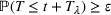
We further illustrate the results of the multiwave SEIRD model by examining the in‐sample fit and out‐of‐sample error in specific states, which we know to have experienced multiple waves. For example, consider the states of Arizona, California, Florida, and Massachusetts. In Figure 1 we see the comparative fit on active cases of the SEIRD and multiwave SEIRD models trained up to September 1, 2020, with the vertical line separating in‐sample and out‐of‐sample predictions. We use vertical green dotted lines to show when the multiwave SEIRD model flagged a new wave. In all of the states, the SEIRD model struggles to match the in‐sample fit, because the structure of the original SEIRD model forces it to average between waves. The curve of a single wave cannot fit the multiwave nature of the data, so the SEIRD model alternates between underestimating and overestimating in‐sample and this results in very inaccurate out‐of‐sample values. However, the multiwave SEIRD model is able to more closely match the in‐sample data, which results in far more accurate out‐of‐sample predictions.

FIGURE 1

SEIRD and multiwave SEIRD in‐sample and out‐of‐sample prediction in Florida, California, Texas, and Massachusetts when trained up to Sept 01, 2020

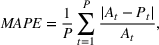
This pattern repeats itself in most of the states where multiple waves occur and over time. For example, Figure 2 shows how the multiwave SEIRD handles the wave that happened at the end of 2020, with results from the models trained up until January 15, 2021. Across states the SEIRD is unable to capture the multiple waves, once again alternating between underestimating and overestimating to average the waves into something that does not describe the actual nature of the pandemic. By comparison, the multiwave SEIRD is again able to more closely match actual cases in‐sample. Out of sample, even though the multiwave SEIRD tends toward overprediction by the end of the test set because it has not learned that wave from the winter holidays is dying off by mid‐February, it is still far more accurate than the SEIRD.

FIGURE 2

SEIRD and multiwave SEIRD in‐sample and out‐of‐sample prediction in Florida, California, Texas, and Massachusetts when trained up to January 15, 2021

It is this structured flexibility of the multiwave SEIRD model that allows it to vastly improve the SEIRD model. By accounting for the multiple waves being experienced in the United States, correctly detecting when they occur and allowing the model to change its parameters accordingly, the multiwave SEIRD model is able to fit the rise and fall of cases in‐sample for accurate out‐of‐sample predictions. Similar graphs for all predicted regions can be found in Appendix S.2.1 and Appendix S.2.1 in Supporting Information.

It is worth noting that the model detects many waves. For example, in California in the January 15 model, the model flags 12 waves. This is a function of the selected lambda, in this case 205. In this work, we present results from selecting lambda based on theoretical results (detection time under a week). For practitioners who are looking to maximize accuracy, we recommend using a validation set to tune the hyperparameter lambda. The higher lambda is, the less sensitive the model will be to changes in infection rate and thus the less waves it is likely to detect. For example, in California, if lambda was increased to 225 or 250, there would have been eight detected waves and if lambda went up to 275, there would have been five detected waves. Table EC.2 in Supporting Information shows the relationship between lambda, the number of detected waves, and out‐of‐sample MAPEs for all modeled regions.

Another way to understand how the multiwave model forecasts COVID‐19 cases is to analyze the relationship between the detected infection rates for each wave,

${\widehat{\beta }}_n^t$

and the mobility during that time. The multiwave model has the ability to detect shifts in infection rate. This change in infection rate could be due to different government interventions (e.g., mask mandates, work from home orders, restaurant/bar closings, gathering size limits), changes in behavior from the population (e.g., compliance with government interventions, resuming or limiting long‐distance travel), or epidemiology‐based differences (e.g., vaccinations, new variants, transmission rate's dependence on temperature). Intuitively, the infection rates for the detected waves,

${\widehat{\beta }}_n^t$

would correlate with several of these drivers.

In order to analyze this relationship, we compiled data on population mobility, government intervention, weather, and holidays. We utilized Google mobility data, which tracked relative changes in mobility for a state in different types of locations (https://www.gstatic.com/covid19/mobility/Global_Mobility_Report.csv). Categories for these mobility scores were retail and recreation, grocery and pharmacy, parks, transit stations, workplaces, and residential. This was combined with state‐level social distancing policies gathered from COVID19StatePolicy Github repository, which tracks government mandates that might affect social distancing and COVID‐19 transmission (https://github.com/COVID19StatePolicy). Examples of tracked policies include emergency declarations, gathering restrictions, school/workplace/restaurant/bar closures, and public mask mandates. We also used historical weather data from National Climatic Data Center (NCDC) of National Oceanic and Atmospheric Administration (NOAA) to get regional temperatures (ftp.ncdc.noaa.gov) and manually flagged relevant holidays that could affect COVID‐19 spread (e.g., Memorial day, Fourth of July, Thanksgiving, Christmas and New Years).

For each state, we created a regularized linear regression using lasso to predict

${\widehat{\beta }}_n^t$

, the infection rate found by the multiwave model, using the features we compiled (mobility, government measures, temperature, and holiday). The regression needed to be highly regularized because there is strong correlation between all of these features. We see the results of the regression for all states in Table S1 in Supporting Information and summarized in Table 4.

TABLE 4

Summary across states of in‐sample and out‐of‐sample r‐squared for lasso predicting infection rates

	In‐sample R‐squared	Out‐of‐sample R‐squared
First Quqartile	0.61	0.49
Average	0.68	0.59
Third quartile	0.78	0.70

With an average out‐of‐sample R‐squared of 0.59, we find that many of the predictors (mobility, government intervention, etc.) can be used in predicting the prevailing infection rate estimated by the multiwave model. This shows another evidence of the correctness of the epidemiological model learnt by the multiwave model.

Benchmark with CDC models

The multiwave SEIRD model is not only strong when considered against the original SEIRD model. We can also analyze these computational results in comparison with the wealth of other COVID‐19 forecasting that has been undertaken in 2020. The CDC has acted as one of the major players in collecting, evaluating, and disseminating COVID‐19 forecasts for cases and deaths. Models that are submitted to the CDC are considered some of the top models in the country. With over 50 models submitted, stemming from academia and industry, these models have a variety of structures and learning processes. Those that follow the epidemiology compartmental structure often significantly change the basic SIR or SEIRD model to account for many subgroups (with some citing over 10 compartments) or make the model's parameters a function of data, such as mobility and government interventions, to help improve accuracy. While this creates strong computational results, it means that these models often struggle to generalize or provide analytical guarantees. By comparison, the multiwave SEIRD model, sticks to the five compartments described in the name and does not incorporate additional features beyond daily COVID‐19 cases and deaths. This simplicity is maintained intentionally to allow for strong and interpretable analytical results in addition to computational results. Despite this fact, we find that the multiwave SEIRD model performs strongly compared to the models uploaded to the CDC. It is because of this strong computational performance that the multiwave SEIRD model is part of the ensemble predictive model, MIT‐CASSANDRA, one of the submitted models to the CDC, and a component of the CDC's ensemble forecast.

In order to compare with CDC models, we simulated the process for submissions to the CDC. Teams must submit models on Monday, and thus only have data up to the Monday of each week, and give predictions for the number of new weekly cases for the next four Fridays. The CDC uses a variety of forecasts, but the primary one is weekly new cases for the United States. Because the SEIRD model is trained at state level and makes daily predictions, we aggregated predictions across the states and days of each week to get incident cases at the national level. Here we show two sample comparisons, the first for models trained up till October 19, 2020, with predictions for October 24, 2020, October 31, 2020, November 7, 2020, and November 14, 2020. The second sample is for models trained up till January 18, 2021, with predictions for January 23, 2021, January 30, 2021, February 6, 2021, and February 13, 2021. We see the results of this comparison in Table 5 and Table 6.

TABLE 5

Multiwave SEIRD and CDC models trained up till October 19, 2020, forecast error and model rank for national weekly incident cases of COVID‐19

	10/24/2020		10/31/2020		11/7/2020		11/14/2020
	MAPE	Rank	MAPE	Rank	MAPE	Rank	MAPE	Rank
CU‐scenario_high	0.163	6	0.160	3	0.209	2	0.267	1
Karlen‐pypm	0.135	4	0.154	2	0.237	3	0.303	2
CU‐nochange	0.166	9	0.179	7	0.250	4	0.304	3
Multiwave SEIRD	0.206	14	0.209	9	0.274	7	0.321	4
CU‐scenario_mid	0.164	7	0.170	4	0.259	5	0.345	5
CU‐select	0.164	8	0.170	5	0.259	6	0.345	6
JHU_CSSE‐DECOM	0.196	12	0.228	11	0.323	10	0.403	7
LNQ‐ens1	0.150	5	0.198	8	0.309	8	0.405	8
UMich‐RidgeTfReg	0.188	11	0.230	12	0.332	12	0.418	9
RobertWalraven‐ESG	0.114	3	0.178	6	0.311	9	0.423	10
CU‐scenario_low	0.173	10	0.213	10	0.326	11	0.431	11
JHUAPL‐Bucky	0.239	17	0.280	14	0.372	13	0.446	12
JCB‐PRM	0.237	16	0.280	15	0.377	15	0.461	13
COVIDhub‐baseline	0.199	13	0.262	13	0.375	14	0.465	14
COVIDhub‐ensemble	0.230	15	0.295	16	0.405	16	0.493	15
$⋮$
TTU‐squider	0.614	24	0.656	23	0.718	23	0.767	22

TABLE 6

Multiwave SEIRD and CDC models trained up till January 18, 2021, forecast error and model rank for national weekly incident cases of COVID‐19

	1/23/2021		1/30/2021		2/6/2021		2/13/2021
Model	MAPE	Rank	MAPE	Rank	MAPE	Rank	MAPE	Rank
UCLA‐SuEIR	0.019	1	0.139	3	0.235	3	0.332	3
Multiwave SEIRD	0.030	2	0.148	4	0.303	4	0.466	6
TTU‐squider	0.055	3	0.071	2	0.098	1	0.126	1
JHU_IDD‐CovidSP	0.101	4	0.001	1	0.141	2	0.283	2
LANL‐GrowthRate	0.106	5	0.198	5	0.327	6	0.476	7
LNQ‐ens1	0.126	6	0.202	6	0.313	5	0.433	4
JHU_CSSE‐DECOM	0.172	7	0.291	7	0.430	8	0.584	9
Geneva‐DetGrowth	0.229	8	–	–	–	–	–	–
Google_Harvard‐CPF	0.242	9	0.439	20	0.585	19	0.851	21
COVIDhub‐baseline	0.266	10	0.363	11	0.493	11	0.644	12
Karlen‐pypm	0.272	11	0.367	12	0.494	12	0.637	11
RobertWalraven‐ESG	0.274	12	0.318	8	0.386	7	0.465	5
COVIDhub‐ensemble	0.287	13	0.358	10	0.477	10	0.613	10
JHUAPL‐Bucky	0.297	14	0.355	9	0.441	9	0.536	8
CU‐nochange	0.309	15	0.393	13	0.550	15	0.726	16
$⋮$
UCSB‐ACTS	0.551	25	0.719	24	0.934	24	1.177	23

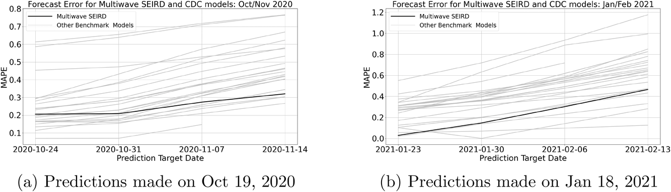
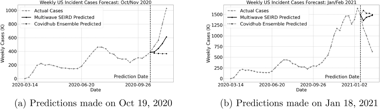
We show these same results visually to highlight the progress of the multiwave SEIRD model's performance over time. In Figure 3 we plot the MAPEs of the CDC models and the multiwave SEIRD over the 4‐week predictions. We see in Figure 3(a) the results for predictions made for October/November 2020, the multiwave SEIRD starts out in the middle of the pack in terms of accuracy, but by the end of the forecast is one of the top performing models. This is because the end of October marked the start of the massive wave that hit the United States over the course of the 2020 fall/winter. Due to its wave detection process and epidemiology structure, the multiwave SEIRD model is able to flag a wave is starting and model the exponential growth in cases. This can be seen clearly when we plot the prediction of the October 19, 2020, model against the true cases and CDC's ensemble prediction in Figure 4(a). The ensemble prediction is the CDC's best estimate of what is going to happen, after considering all of the submitted CDC models, and represents its official forecast. We see that the CDC ensemble model predicts a flat curve for new cases, having not picked up yet on the scale of the new wave, while the multiwave SEIRD has begun to model the exponential growth.

FIGURE 3

Multiwave SEIRD and CDC models forecast error for national weekly incident cases of COVID‐19

FIGURE 4

Multiwave SEIRD and CDC ensemble forecasts for national incident cases of COVID‐19

The predictions made on January 18, 2021 are a little more interesting. Here we see that all the models are struggling to forecast what is going to happen, with MAPEs for all models unusually high. The United States was at a tipping point and it was possible the cases would continue to grow or start dying off. This is clearly shown when we look at the state‐level predictions in Figure 2. Some states have already begun to pivot down and cases have started dying off, but other states look like they were going to grow. For the multiwave SEIRD model, this means that some states have forecasts that show exponential decay, while others continue to show exponential growth. We can see this tension in the national forecasts made by the multiwave SEIRD in Figure 4(b), as the forecasts show some drop, but then growth again. However, because the SEIRD model is able to flag that the wave was dying off in enough states, it starts off closer to the truth in the first week of predictions, and this translates to strong performance across the rest of the weeks, resulting in the multiwave SEIRD model being among the most accurate models during this time, as shown in Figure 3(b).

CONCLUSIONS

The COVID‐19 pandemic has shown us that disease transmission is not determined just by how contagious a virus is. Population behavior and mitigation strategies play a major role in how quickly a disease spreads. Because of this, it is not enough to just model a virus's contagion and assume that population behavior remains constant. The multiwave SIR model creates a basis for understanding, modeling, and predicting when epidemics are driven by human nature as much as a virus's transmission rate.

The multiwave SIR model accounts for the multiple waves of COVID‐19 seen in the United States. The model provides a framework for detecting when a new wave is occurring, and allows the epidemiology model the flexibility to adjust for new waves. The detection process is theoretically proven to be rigorous, namely, quick to pick up on new waves. Experimentally, the multiwave SIR model shows significant improvement over its single‐wave counterpart. In regions that have experienced multiple waves, the multiwave SIR model is not forced to average between them like the original SIR model, but rather can match each wave for its infection/transmission/recovery rates. This results in significantly better in‐sample fit and out‐of‐sample accuracy.

Forecasting the COVID‐19 evolution, and specifically the occurrences of new waves, is critical in managing operations and supply chains through the pandemic. Identifying and forecasting COVID‐19 waves is crucial in answering three major supply‐chain related questions for manufacturers, retail companies, restaurants, and health care organizations: (i) What products and resources should these organizations supply? (ii) How should these organizations structure their supply chain in times of pandemic? (iii) What medium should these organizations use to sell or distribute their products? Alternatively, (i) What to supply? (ii) How to supply? and (iii) How to distribute?

• 1.

What to supply?: the first point is about shifting priorities and changing customer behavior. New waves appearing trigger a panic‐buying behavior. As a result, there is a demand surge for many essential supplies such as groceries or hygiene products at common point‐of‐sale locations (Adulyasak et al., 2020). Being able to correctly predict new waves in particular locations allows organizations such as retailers to anticipate this demand surge and provide enough supply to avoid letting the hoarding behavior put the most vulnerable people at risk. This is also true in a healthcare setting, when hospitals in different locations experience a demand surge in resources like ventilators when a new wave of COVID‐19 hits (Bertsimas et al., 2021), requiring a rapid shift in the way these resources are allocated.

2.

How to supply?: additionally, the supply chain during a pandemic should satisfy two main criteria: safety and flexibility. For the former, recent research such as Xu et al. (2020) and Mollenkopf et al. (2020) shows how the COVID‐19 spread impacts the supply chain through the safety measures, and how to make these safety measures evolve accordingly. For the latter, as governments tighten or loosen the COVID‐19 restrictions according to new waves appearing, forecasting models with high predictive power such as the multiwave SIR allow specific businesses such as restaurants to anticipate the reopening and closure of their activities. Thanks to that, these businesses can plan the dependant supply chains subsequently, for example, by prioritizing diversification or limiting large inventories of perishables when a new wave is approaching. Finally, there have been a lot of literature on resource allocation during pandemics based on these dynamics, whether it is for general resources (Long et al., 2018) or vaccine for example (Teytelman & Larson, 2013), where similar predictions are used in optimization‐based models.

3.

How to distribute?: last but not least, as online retail jumped to $26.7 trillion in 2020, up 4% from the previous year (UNCTD, 2021), fueled by COVID‐19, retailers, for example, in clothing or home furniture, need to be able to accommodate different distribution channels. The supply chain should shift to online retail during lockdowns and when new waves appear, and allow the safe reopening of brick‐and‐mortar stores when restrictions are loosened and demand for in‐person shopping increases.

This allows us to conclude that the multiwave SIR model, combined with the right optimization framework, can be used to drive meaningful real‐world impact.

Footnotes

ACKNOWLEDGMENTS

The authors would like to thank MIT's Quest for Intelligence for their generous support both in terms of funding but also in terms of research that allowed this paper to become possible. A special thanks to Akarsh Garg and Shane Weisberg for their help on the computational parts of this work. The authors would also like to thank the review team for their insightful comments that helped us improve both the content and exposition of this work.

ORCID

Georgia Perakis

Divya Singhvi

Omar Skali Lami

Leann Thayaparan