
Abstract
Improving access to family planning services is key to achieving many of the United Nations sustainable development goals. To scale up access in remote areas and urban slums, many developing countries deploy mobile family planning teams that visit “outreach sites” several times per year. Visit frequencies have a significant effect on the total number of clients served and hence the impact of the outreach program. Using a large dataset of visits in Madagascar, Uganda, and Zimbabwe, our study models the relationship between the number of clients seen during a visit and the time since the last visit and uses this model to analyze the characteristics of optimal frequencies. We use the latter to develop simple frequency policies for practical use, prove bounds on the worst‐case optimality gap, and test the impact of the policies with a simulation model. Our main finding is that despite the complexity of the frequency optimization problem, simple policies yield near‐optimal results. This holds even when few data are available and when the relationship between client volume and the time since the last visit is misspecified or substantially biased. The simulation for Uganda shows a potential increase in client numbers of between 7% and 10%, which corresponds to more than 12,000 additional families to whom family planning services could be provided. Our results can assist policymakers in determining when to start data‐driven frequency determination and which policies to implement.
Introduction
Access to family planning plays a crucial role in achieving many of the United Nations (UN) sustainable development goals (Starbird et al. 2016), notably goal 3 (good health and well‐being) by preventing maternal deaths and controlling the spacing of pregnancies. Universal access to contraception is estimated to reduce unintended pregnancies by 75%, maternal deaths by 25% (Darroch et al. 2017), and infant mortality by 10% (Cleland et al. 2006). Additionally, family planning allows women to postpone the birth of their first child and advance their education, which aids goals 4 (quality education), 1 (no poverty), and 5 (gender equality). For example, if adolescent girls in Brazil and India could postpone childbearing until their early twenties, the economic productivity of those countries would increase by more than US$3.5 billion and US$7.7 billion, respectively (UNFPA 2014). The UN estimates that, for “every dollar spent in family planning, between two and six dollars can be saved in interventions aimed at achieving other development goals” (UN Population Division 2009).
Despite these compelling facts, for at least one out of five women 1 in Sub‐Saharan Africa the need for family planning goes unmet (United Nations 2015) 2 . Many live in rural areas and urban slums, where access to family planning is limited or non‐existent (Eva and Ngo 2010, Solo and Bruce 2010). Mobile (i.e., traveling) outreach teams are crucial to scale up access to family planning in these areas. Yet with a widening gap in funding of family planning organizations (UNFPA 2018), mobile services have to reach more people with fewer resources.
Mobile teams, consisting of doctors and nurses, are often the only provider of family planning services and have to allocate time to the sites in the catchment area. Naturally, they tend to visit sites that attract many clients more often than those that attract relatively few. Marie Stopes International (MSI), an NGO with 500 mobile family planning teams, has therefore introduced the guideline that (besides other factors) “The level of client demand […] should be used to determine the optimal frequency of visits” (MSI 2016). Although this guideline is intuitive, it is loosely specified. Our interviews with outreach leads from five African countries show that country programs interpret these guidelines in different ways, and our data analyses reveal that adherence to them is low. This, as our study shows, has a negative impact on client volumes per outreach day, used in this study as the metric of effectiveness.
Developing more firmly specified policies is a necessary but difficult task. Policies not only depend on client numbers but affect client numbers: More frequent site visits may lead to fewer clients per visit. In the absence of research on this effect, however, this has so far not been factored into decisions on visit frequency. Our study thus focuses on the frequency determination problem (FDP):
Given a team, a set of sites, a lower and an upper bound on the frequency of visits to each site, and a certain number of service delivery days per month, what frequencies should be assigned to each site so as to maximize the effectiveness of the visits?
We use a large dataset from MSI to fit a fixed‐effects model that captures the link between effectiveness and visit frequency. We then mathematically model FDP and analyze this model to obtain characteristics of optimal frequencies. Although the latter can be efficiently calculated by algorithms, there are strong arguments for basing frequency decisions on simple policies. We therefore use the characteristics of optimal frequencies to develop practical frequency policies and test them using a simulation of MSI's mobile teams in Uganda. Our findings were discussed with staff at MSI headquarters in London and with the Marie Stopes Uganda team.
The main finding is that, despite the complexity of the frequency optimization problem, simple visit frequency policies yield near‐optimal results. This holds even when little data is available, parameter estimates are substantially biased, and the objective function is misspecified, and even though several simplifying assumptions are made. Based on the data for Marie Stopes Uganda, we estimate that putting these policies in place could increase client numbers by between 7% and 10%. If this were representative of MSI as a whole, an increase of 7% would correspond to at least 175,000 clients globally 3 . In a context of severely reduced funding, such an increase in effectiveness would go some way to achieving the UN sustainable development goals.
Our paper is organized as follows. Section 2 gives further details on the way mobile teams operate and the FDP. Section 3 discusses the relevant literature. In Section 4, we develop an econometric model for client numbers to examine the effect of visit frequencies on the number of clients per visit. In Section 5, we formally model and analyze the FDP and propose exact solution methods and policies. Section 6 presents numerical results on the effectiveness of the policies for Marie Stopes Uganda.
Problem Description
This section describes the FDP faced by outreach teams. This was obtained through discussions with outreach leads from five countries in which MSI operates, the international outreach lead and the directors of the research team.
Each outreach team has a fixed set of sites which it visits regularly to deliver family planning services, determined in cooperation with the government. These are often small healthcare facilities that do not provide (long‐term) family planning methods. They also use pop‐up tents. Teams provide short‐term and long‐term family planning methods as well as counselling, treatment of side effects, and implant and intrauterine device (IUD) removal. Some also offer permanent methods of contraception (i.e., sterilization).
Each team has a limited number of days per month to visit sites. Nearly all site visits last a full day. Sometimes two neighboring sites can be visited on the same day. In most countries, the visits are day trips that start and end at the team's base, but they may camp on site to reach remote locations on multi‐day trips. Before the visit, marketing or “demand generation” is done through radio, posters, or community health workers to encourage people to come. During the visit, drivers sometimes tour the village with a megaphone to announce that the team is on site. Since demand generation typically occurs locally and travel times between sites in rural areas are typically long, clients rarely come from different sites.
Client volumes per site visit are determined by factors such as the intensity of demand generation, staffing, the service package, whether a market‐day or vaccination campaign is taking place, the time of arrival/departure, and visit frequencies. We focus on optimizing the latter. MSI recognizes its importance in its guideline “The level of client demand […] should be used to determine the optimal frequency of visits” (MSI 2016). Similarly, USAID's “handbook for program planners” for mobile outreach services mentions selecting “frequency of mobile outreach services” as the second program decision (after selecting sites to be visited) and states that the optimal frequency “will depend on demand for services” (Solo and Bruce 2010).
Visit frequencies determine the “return time,” or the time between visits. They should take into account ethical and medical considerations, since it is neither fair nor medically advisable to have long return times. Clients may want to have a contraceptive device replaced or removed or require treatment for a side effect. MSI has set an interval between visits of no more than 6 months. They can be flexible on return times only if government providers can assure removal of contraceptive devices and provide access to short‐term methods such as condoms. If not, they aim for a return time of 3 months at most. Our analyses assume a 6‐month upper bound. There is a minimum interval between visits as it takes about a month to generate sufficient demand and coordinate the visit with those managing the local facilities.
These bounds leave room to optimize visit frequencies. Although it makes sense to visit sites that attract many clients more often, this has not yet been translated into a concrete policy. Should a site that attracts twice as many clients be visited twice as often? What would higher visit frequencies look like? How far should it depend on historic frequencies? Questions such as these are presently unanswered.
Perhaps unsurprisingly, many teams link their return times to demand in a relatively ad hoc way. Data from Marie Stopes Uganda show that for those sites with return times below the 6‐month upper bound, there is little to no alignment with client numbers (as illustrated in Figure 1). There are quite a few sites with a long return time but a large number of clients. Conversely, many sites have low average client numbers but are visited frequently. Shifting resources from sites with short return times and low average client numbers to those with longer return times and higher numbers would seem likely to improve effectiveness (measured as the average client volume per outreach day).
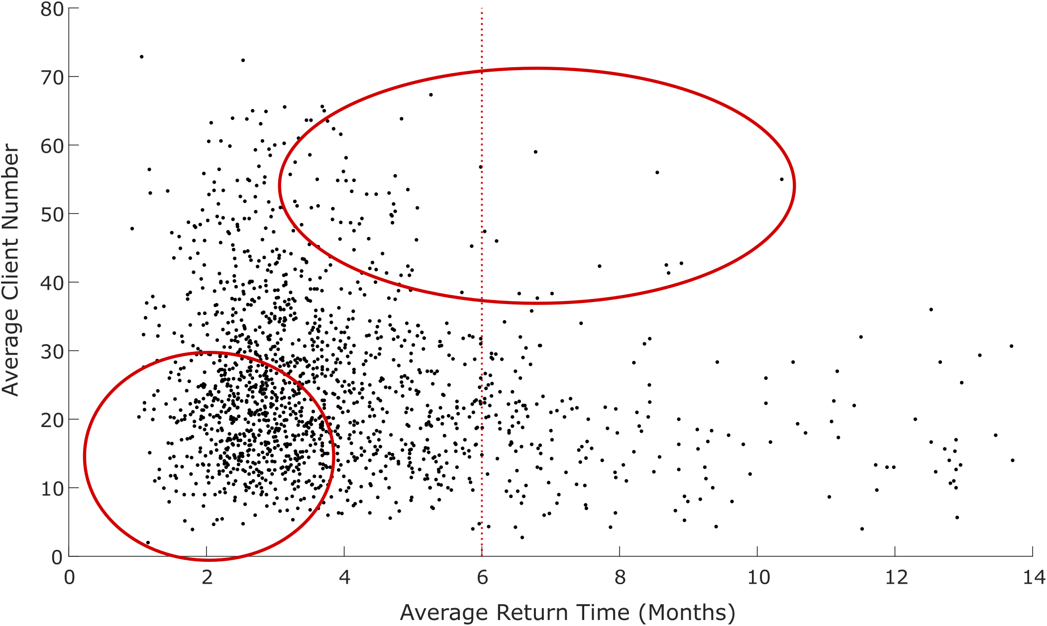
Current Alignment of Return Time with Demand. Each Dot Represents a Site. The Bottom Left Circle Highlights Sites with a Low Client Volume and Low Average Return Time. The Other Circle Highlights Sites with a High Client Volume and High Average Return Time. Shifting Resources from the Former to the Latter would Seem Likely to Improve Effectiveness. [Color figure can be viewed at
To optimize frequency policies, it is key to understand how return times affect client volumes. Our conversations with MSI staff suggest that client numbers tend to increase with an increase in return time, which was attributed to more time for demand‐generation, word‐of‐mouth effects, and existing clients demanding contraceptive device renewals or removals. However, the strength of this effect may be limited. For example, adequate demand‐generation can result in substantial client volumes irrespective of the return time. Long return times were said to reduce client satisfaction and induce a loss of trust in the teams, which also suggests that the effect diminishes at some point. More specific evidence on the effect of return time on client numbers is lacking (an issue addressed in Section 4).
The effectiveness of simple policies as opposed to advanced algorithms is also unclear. Despite the complexity of the FDP, organizations such as MSI have good reason to prefer simple policies, the main one being that they fit with the prevailing decentralized decision‐making culture. Another is that advanced algorithms push up the costs of implementation, roll‐out, and training (De Vries and Van Wassenhove 2020). Organizations also value flexibility, that is, policies that simply recommend a frequency and leave the teams to decide on day‐to‐day planning. For this reason, the policies proposed in this study only recommend frequencies, allowing each team to incorporate local knowledge into its decision making. For example, MSI team leaders know when it is market day in a village, which tends to lead to higher numbers of clients. According to Peter Schaffler, MSI's outreach lead, “Team leaders are also extremely aware of road conditions and incorporate this knowledge into their routing decisions” (personal communication, May 1, 2018). Section 6 analyses the optimality gap of visit frequency policies.
A third question considered is how the effectiveness of a policy depends on the amount of data available. MSI started systematic data collection in Uganda in 2015. Other countries started more recently, so few data points are available. This can be perceived as a barrier to data‐driven decision making. We analyze the impact of data quantity in Section 6.
Based on discussions with MSI, we have chosen to analyze policies in terms of numbers of clients per outreach day. One alternative measure would be to use the total couple years of protection (CYPs) provided per outreach day. The CYPs of a particular contraceptive method is the number of years that it protects a couple from an unwanted pregnancy. Another measure could be weighted client numbers depending on specific target groups: the young, the poor, and clients who have no other way to access family planning. This would take into account that seeing 20 clients in a relatively wealthy, well‐served site is not the same as seeing the same number of clients at a poorer, remote, underserved site. The main reason for our choice (clients per outreach day) is that it fits the way outreach teams presently make decisions. The policies we encountered during our interviews were all expressed in terms of client numbers. Marie Stopes Madagascar, for example, aims to carry out monthly visits for sites that attract on average more than 20 clients per visit. Maximizing client volumes also fits well with maximizing CYPs and weighted client volumes, since differences between sites in the same catchment area in terms of either CYPs or the percentage of clients in each target group are small. In Section 6.2, we examine how the performance of our policies is affected by this choice.
Literature
Three streams of literature are closely related to our work: mobile (family planning) outreach, global health operations management, and related scheduling problems. The FDP most closely resembles a knapsack problem (KP) with a separable concave non‐linear objective function and linear constraints (see Ibaraki and Katoh 1988, for an overview of solution algorithms). In particular, the FDP can be modeled as a KP where all items have the same weight, the objective value is a non‐linear function of the number of a given item included (i.e., the visit frequency), and this number is bounded from above and below. The specific objective function of the FDP is what makes this problem distinctive.
Mobile family planning units have been shown to significantly affect contraceptive use. Using data from Zambia, White and Speizer (2007) estimate that the modern contraceptive prevalence rate in rural areas would increase by 5.9 percentage points if all women had at least one outreach visit. Joshi and Schultz (2013) study the impact of introducing outreach services in villages in Bangladesh, and show substantial benefits in terms of birth spacing and fertility rates in comparison to “control villages.” Similarly, Lutalo et al. (2010) use a randomized controlled trial in Uganda to show that introducing outreach services increases the use of hormonal contraceptives and decreases pregnancy rates. Outreach has also been shown to increase adoption of long‐term family planning methods and reach poor and underserved populations (Ngo et al. 2017, Noccio and Reichwein 2013).
Access to and impact of family planning is commonly measured through indicators such as (modern) contraceptive prevalence, unmet need, the number of unintended pregnancies, unsafe abortions, and maternal deaths averted, and adult birth rates (cf. FP2020 2020). Since is it hard and time‐consuming to measure site‐level changes in these indicators, mobile outreach programs commonly use service statistics such as the number of (young) clients served, the number of adopters (i.e., clients who (re)started using contraception), and CYPs (cf. Ngo et al. 2017). Weinberger et al. (2013) propose a model to translate these statistics into an estimated impact on contraceptive prevalence.
Though a significant body of research has covered impact of mobile family planning, little is known about impact drivers. This study contributes to the literature on mobile (family planning) outreach by exploring how visit frequencies affect client volumes and how to incorporate this in visit frequency policies.
We identified five OR/MS papers that specifically consider the deployment of mobile healthcare units when capacity is restricted. Deo et al. (2013) study mobile asthma care units that visit schools, taking the timing of visits as given, and optimize the scheduling of patients to maximize health gains. Our work is similar in that we also consider (a proxy of) outcomes, but differs in that we consider optimizing the frequency of visits. Hodgson et al. (1998) and Doerner et al. (2007) do consider the scheduling of site visits, and model this as a covering tour problem (CTP). The aim is to construct a tour through a subset of locations in a network, subject to the constraint that a pre‐specified percentage of the population (or the locations considered) must be within a given distance from a location in the tour. There are two structural differences between the CTP and the FDP. First, a CTP does not consider optimizing visit frequencies, nor how demand is dependent on frequency. Second, the objective of a CTP is to minimize travel time, whereas we aim to maximize the number of clients reached in a setting where outreach teams use one‐day trips to visit sites.
McCoy and Lee (2014) consider the allocation of motorbike visits to outreach sites, with the objective being to maximize effectiveness and fairness. Each site visit is said to satisfy a certain “need.” Effectiveness is defined as the total “need” satisfied. Fairness is incorporated by assuming diminishing utility of additional visits to a site. The authors quantify these objectives as a weighted sum of the number of visits to each site, raised to the power of some constant. As detailed later, the functional form of our objective function is different and fits with the data from MSI. Unlike them, we also consider lower and upper bounds on the number of visits. We focus on policies and insight into the effectiveness of family planning operations, whereas they focus mainly on analytical insights into optimal allocation decisions.
De Vries et al. (2021) analyze the scheduling problem for mobile teams in medical screening. The problem clusters villages that can be easily incorporated into a daily schedule in terms of the travelling distance between them. It then assigns each mobile team to one cluster in each planning period. A key difference is that they consider how to optimize schedules (i.e., which sites to visit in which month), whereas our work considers the more tactical question of how to design frequency policies. They consider a curve describing how health evolves between visits; their objective is to minimize the total expected disease burden over the planning horizon, that is, the area under the curve. In contrast, we consider the specific value of the curve for each visit, namely the number of clients. As a consequence, the functional form of the objective function differs. As in this study, De Vries et al. (2021) consider both optimal solution approaches and planning rules.
Maintenance scheduling problems (MSPs) consider a fixed number of machines to be maintained and a maximum number of maintenance visits in a given period of time (see Nicolai and Dekker (2008) for a review). If we substitute machines for sites and maintenance visits for site visits, the similarities are clear. However, the objective function is substantially different. In addition, our focus is on the development of simple policies, whereas the MSP literature typically considers exact approaches.
Data Description and Analysis
This section describes the data used in this study and analyses the effect of return time (the time since the last visit) on client numbers. The results are used in the modeling of the FDP in Section 5 and in the case study in Section 6.
Data Description
We use data on outreach visits from MSI. MSI is exceptional in the sense that it is one of the few humanitarian organizations to systematically capture data on operations and use it to improve policies, guidelines, and operations.
We use data from Marie Stopes Uganda from May 2015 to September 2017, from Marie Stopes Madagascar from January 2016 to March 2018, and from Marie Stopes Zimbabwe from January 2017 to September 2017. These countries were chosen by MSI because the data were of good quality. The start dates correspond to the start of systematic data gathering and the end dates to the time that access to the data was terminated. The cleaned datasets for Uganda, Madagascar, and Zimbabwe include 10,293 visits to 1581 sites, 10,498 visits to 1794 sites, and 732 visits to 243 sites, respectively. For each site visit, the datasets show the name of the site, the date, the team, and a list of clients. For each client, they list among others the age bracket, number of children, and the family planning method. We use this data to determine the total client volume and the return time in months for each site visit. Descriptive statistics are presented in Table 1.
Descriptive Statistics of the Datasets
For each site, the first visit included in the data is excluded, because the return time is unknown. We also exclude all sites that have only one visit for which return time is known. This excludes 23%, 46%, and 71% of the sites for Uganda, Madagascar, and Zimbabwe, respectively. With the Uganda data, we exclude visits where multiple teams go to the same site. These visits represent special events, such as youth focus days, which result in unusually high numbers of clients. Some exceptionally high numbers are also observed in Zimbabwe. Based on our conversations with MSI staff, we set the cut‐off value for the number of clients that can realistically be seen by one team to 120. We exclude the 3.5% of visits that exceed this threshold. From the Madagascar data, we exclude the 0.4% of visits where no family planning methods are provided, because these are special events such as AIDS prevention or vaccination campaigns.
Effect of Return Time on Client Numbers
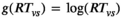
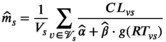
In this section, we aim to model the effect of the return time for visit v to site s, 


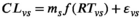
Here 


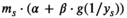
As stressed during conversations with MSI outreach leads for Madagascar, Tanzania, and Sierra Leone and with HQ staff (see Section 2), client numbers are determined by many factors that are not related to return time, such as the population density of the area and marketing efforts. We therefore split 
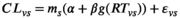
Here, α and β are non‐negative constants. We estimate both parameters for Uganda, Madagascar, and Zimbabwe. The larger β, the more client numbers grow in return time, possibly because of word of mouth, community health workers, or renewals. α will indicate the percentage of clients reached when 


The formulation reflects the implicit assumption that client numbers for different sites are mutually independent. As the distances between sites are large and use of health services tends to drop off sharply the farther clients have to travel, this assumption is realistic (see, e.g., Tanser et al. (2006)). Another implicit assumption is that the effect of return time is proportional to 
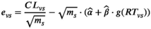
Appendix A describes how we fit function (2) and how we deal with endogeneity (site characteristics affect return times) and heteroskedasticity (the variation in client volumes is larger for sites that attract more clients). In short, to handle endogeneity in return times, we first estimate β by relating within‐site variations in return times to within‐site variations in client volumes. Plugging this estimate into function (2), we estimate α and 


Results
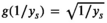
Estimated WLS Parameters (Standard Error between Parentheses), Root Mean Squared Error of Calibration (RMSEC), Mean Absolute Error (MAE), and Root Mean Squared Error of Prediction (RMSEP) for Multiple Functional Forms


Notes
All parameters are significant at a 1% significance level.
Lowest value among the functional forms in bold.


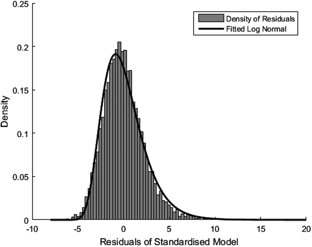
Shifted Log Normal Distribution Fitted to Errors for Uganda
We can summarize our findings as follows. First, the results indicate that the effect of return time on client numbers is statistically significant and positive for all the countries considered. Second, return time has a relatively limited effect on client numbers. Finally, we showed the error terms to approximately follow a log‐normal distribution. The relations identified in this section will be used in the modeling of the FDP in Section 5 and in the case study in Section 6.
Model and Solution Methods
This section has three objectives: to derive insights on determinants of optimal visit frequencies, to develop methods to determine optimal frequencies, and to explain various (heuristic) policies for choosing visit frequencies. In Section 5.1, we formally model the FDP. Section 5.2 develops algorithms to solve the model and Section 5.3 analyses the resulting frequencies. In Section 5.4, we use insights from the algorithms developed in Section 5.3 to develop several frequency policies.
Model
The model considers one outreach team and a set of outreach sites 


We assume that the 


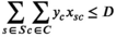
The FDP can then be modeled as in model (M1). The objective (4a) maximizes the total expected number of clients reached in a month. Capacity constraint (4b) restricts the total number of visits, and (4c) and (4d) are boundary constraints.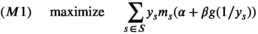
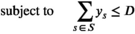
Problem (M1) is a non‐linear simple allocation problem with boundary constraints (Derman 1959). Throughout this study, we consider the typical case when 


Solution Algorithms
In this section, we explain the algorithms used to solve (M1) to optimality for multiple functions 


Client Numbers Independent of Return Time
When client numbers are independent of return time and 
In short, we initially set all visit frequencies at the lower bound. That leaves 


Client Numbers Linearly Dependent on Return Time
If client numbers are linearly dependent on return time, that is, 

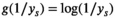
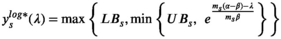
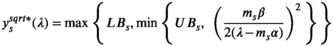
Client Numbers Non‐Linearly Dependent on Return Time
Under a logarithmic dependency 

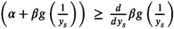
Applying Lagrange relaxation leads to 


Numerical Insights into Optimal Visit Frequencies
The algorithms in Sections 5.2.1 and 5.2.2 provide a valuable insight: There is at most one site with an optimal frequency different from the lower or upper bound if 

In particular, we assess to what extent optimal solutions resemble lower and upper bound frequencies and how this depends on context. We specifically consider three contextual factors. The first is the magnitude of the effect of return time on client numbers, i.e., the value of the parameter β. We compare optimal frequencies for the values of β fitted for Uganda and Madagascar in Section 4, since these values were the highest and lowest, respectively. Second, we examine how frequencies are affected by the level of variation in 
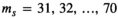
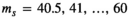


We compute the optimal frequencies for each instance using 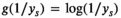
Frequencies of Sites in Several Instances under 


Table 3 shows that for several sites the frequencies are not set to the bounds. This happens more frequently in Uganda than in Madagascar. The reason is that the value of β is higher for Uganda. The higher the value of β, the greater the increase in client numbers on the return visit. The model then “deviates” more from the constant model, where it is optimal to set frequencies to the bounds. Additionally, the numbers show that a larger variation in 


In Online Appendix E, we also show that frequencies that are not on the bounds are about equally distributed across the interval [LB, UB]. That is, they are not concentrated around the bounds. This suggests that it is beneficial to develop frequency policies which allow for at least one frequency value between the bounds.
Finally, the number of sites for which the assigned frequency is not on the upper or lower bound does not seem to depend strongly on capacity. In all instances, a decrease in capacity of 40 days makes hardly any change to this. In short, under a logarithmic effect of return time on client numbers, the optimal frequencies seem to differ most strongly from the bounds when the variation in 
Policies
In this section, we use insights from Section 5.3 to develop frequency policies. All our data‐driven policies rely on an estimate of the site‐specific multiplier 


This is an unbiased estimator that assumes client numbers 
Given a choice on how to estimate 


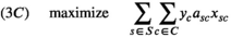
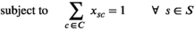
Such guideline on the percentage of sites in MFC can, for instance, be developed by solving model (3C), which models the problem of allocating sites to frequency categories. Here we define 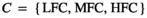


Optimality Gaps
We now analytically prove a bound on the optimality gap when using two frequency categories instead of infinitely many and then generalize this to the case when k frequency categories are distinguished. We specifically consider the realistic case when 
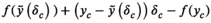
Objective function (4a) is concave in 


In addition, we consider the realistic scenario when visiting a site more frequently never leads to fewer clients in that site in total and state without proof (it follows when applying the product rule) that:
bjective function (4a) is non‐decreasing in 
We note that, for the fitted values of α and β presented in Section 4.3, this condition is always met.
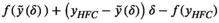
Let us write the objective function again as 


The optimality gap of TwoCP, measured as the absolute difference with the optimal InfCP solution value, is bounded from above by 
We refer to Appendix B for the proof, which utilizes the two conditions stated in Lemmas 1 and 2. Specifically, we replace the objective function by a linear “outer approximation.” The optimal solution is the same as the TwoCP solution and its value provides an upperbound on the optimal solution value. Taking the difference between this value and the “real” value of the TwoCP solution yields the optimality gap. We apply the same approach to generalize the result to the case when there are k frequency categories.
The optimality gap of a policy that distinguishes k frequency categories, measured as the absolute difference with the optimal InfCP solution value, is bounded from above by 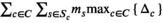


For the case study presented in the next section, with 
We do note that these results are obtained for the case when the decision maker knows the exact value of 
Case Study: Outreach Teams of Marie Stopes Uganda
In this section, we study the performance of the policies proposed in Section 5.4, using Marie Stopes Uganda as a case study. We use real data from 10,293 visits to 1581 sites in Uganda. We first explain the simulation model before presenting the results.
Simulation Model
The simulation model uses function (2) with the parameters α, β, 


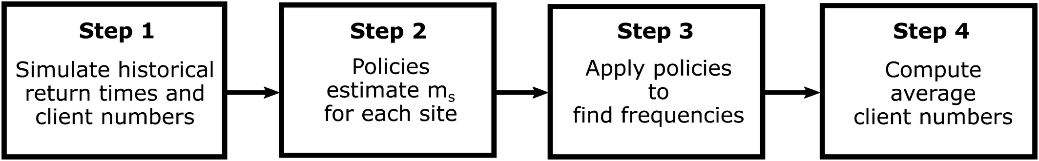
Overview of Simulation
Simulation Results
We first assess the trade‐off between the complexity and effectiveness of policies when historical return times are used in Step 1. Second, we analyze how the effectiveness of the policies depends on the amount of historical data available for each site. Third, we analyze the sensitivity of results to different simulated return times.

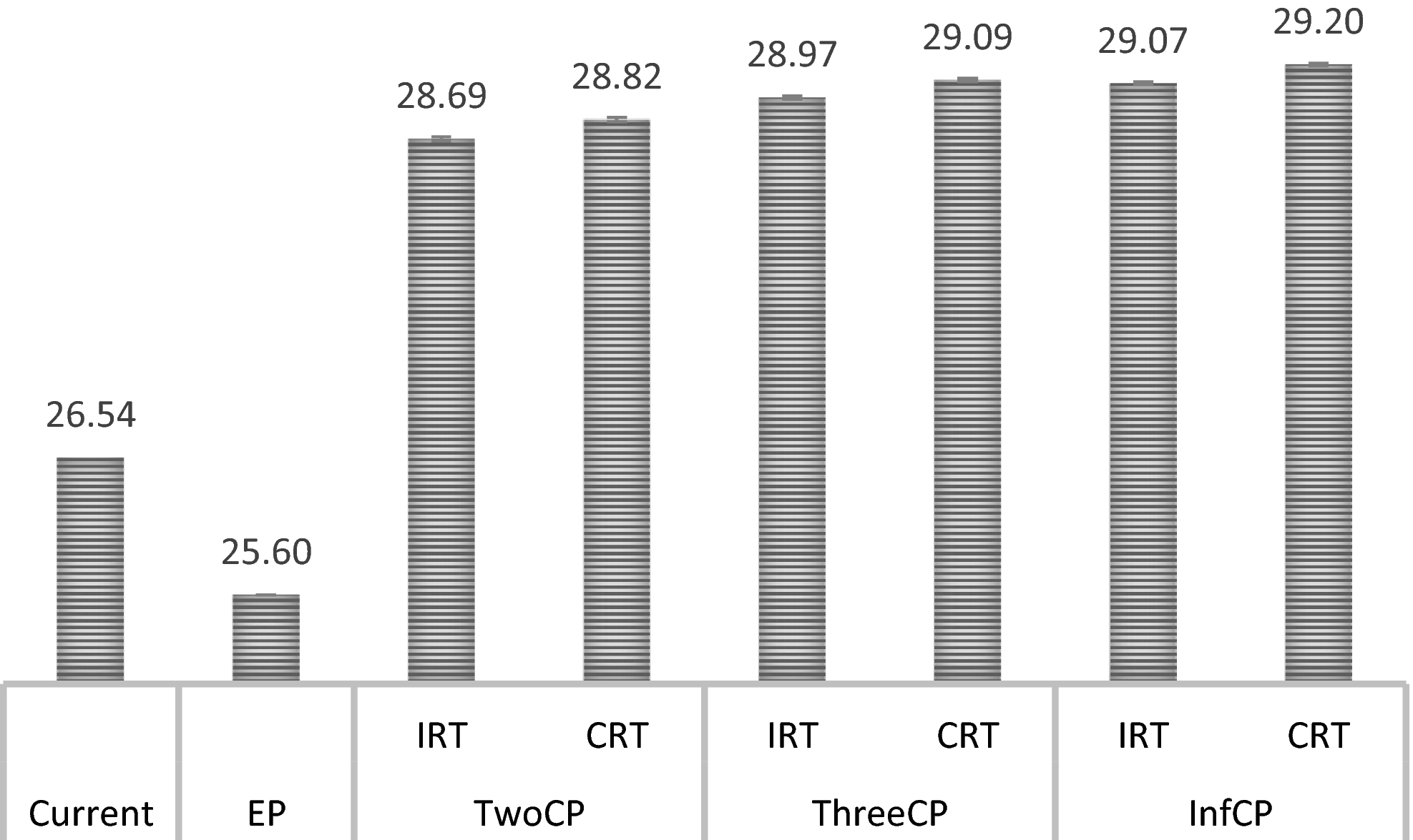
Average Number of Clients Per Visit of Policies for n = 5, Including 95% Confidence Interval (width < 0.03 for Each Policy)
Although the increases in client numbers might seem small, even a small increase per visit mean that, over the course of a year an enormous number of additional families can be provided with family planning services. With D = 20 and 24 teams, the increase in client numbers when moving from the current situation to TwoCP‐IRT corresponds to an increase of over 12,000 clients a year in Uganda alone.

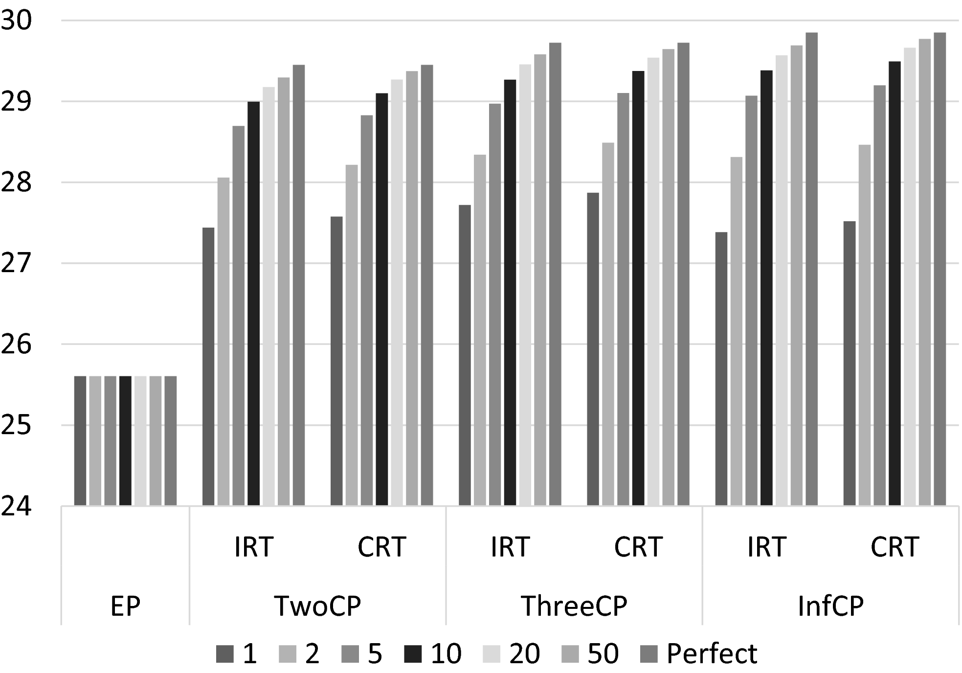
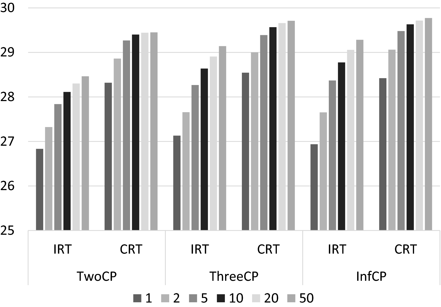
Average Number of Clients Per Visit for Multiple Values of n and all Policies
Even with n = 1, all policies outperform the EP by at least 3%. The ThreeCP consistently performs around 1% better than the TwoCP. It is interesting that the InfCP performs worse than the TwoCP and ThreeCP if n = 1. The policy appears to assign frequencies that are too specific, based on too little information. The InfCP only outperforms the ThreeCP when n ≥ 5. With perfect information, the TwoCP results in 11% more clients than is currently the case, the ThreeCP in close to 1% more clients than the TwoCP, and the InfCP in less than 0.5% more than the ThreeCP. The effect of correcting for return time diminishes with n from around 0.5% when n = 1 to around 0.25% when n = 50.
Average Number of Clients Per Visit for Multiple Values of n and All Policies when Using Policy Return Times in Step 1
These results can be explained by the observation that the variation in client numbers will decrease when mobile teams start using frequency policies. This happens because sites with a high 


Sensitivity Analyses
Our analyses and policies implicitly make several simplifying assumptions. This section summarizes the results of extensive sensitivity analyses presented in Online Appendix G.


Conclusion and Discussion
Mobile outreach teams are crucial to scale up access to family planning in rural areas and urban slums. Gaps in funding mean that mobile teams have to reach more people with fewer resources, without sacrificing the quality of the service. This study contributes to this endeavor by studying the frequency determination problem (FDP) or how to determine site visit frequencies for mobile outreach teams in order to maximize client volume per outreach day. Visit frequencies have an upper and lower bound based on medical, ethical, and planning concerns and are further constrained by the number of days each mobile team is available for site visits. We specifically consider the FDP in the context of family planning and use data from Marie Stopes International (MSI).
The complexity of the FDP lies in how the frequency of site visits affects client numbers, specifically through the return time (i.e., the time since the last visit). We use MSI data for three different countries to analyze the strength of this effect. We find that the client numbers are higher when the return time is longer, but that the magnitude of this effect differs across the countries considered. For example, we estimate that increasing the return time from one month to six months increases the expected client volume by 6%, 35%, and 27% for Madagascar, Uganda, and Zimbabwe, respectively.
We examine how optimal frequencies depend on the shape and magnitude of the effect of return time on client numbers. When client numbers are non‐linearly dependent on return times (we consider a logarithmic and square root shape), the optimal frequencies can be largely on the bounds, depending on various factors. They deviate widely from the bounds when the effect of return time on client numbers is large—that is, when demand progresses strongly over time—such that the objective function differs most strongly from the linear case. Deviations from bounds are also more frequent when there is only a small variation in the so‐called baseline client volume—the expected client volume for a given baseline return time. In extreme cases, when all sites have the same baseline client volume or when demand increases very strongly with the return time, it can be optimal to set none of the frequencies to the bounds. These results have important implications for outreach program managers. First, they show that in none of the realistic functional forms and parameter settings considered it is optimal to only have one frequency category (i.e., to assign the same frequency to each site). Second, they indicate when it is beneficial to have three or more frequency categories: when demand progresses strongly over time and when there are large variations in baseline client volumes across sites.
We used these insights to develop simple frequency policies that use only two (TwoCP) or three (ThreeCP) different frequencies and present analytical results on their worst‐case performance for the case when decision makers know the exact value of the baseline value of each site. For our case study on Marie Stopes Uganda, they reveal a worst‐case optimality gap of 7.7% for TwoCP and 4.0% for ThreeCP. This is an important finding, as a large optimality cap could be seen as a barrier to adoption of the policies.
We also tested the policies’ effectiveness in an extensive simulation analysis for Marie Stopes Uganda. The main takeaway for outreach program managers is that the effectiveness of mobile teams can increase substantially when visit frequencies are based on historical client numbers. We estimate that the expected number of clients can increase by over 7% compared to the current number when using policies that base visit frequencies on historic client numbers. An increase on this scale would correspond to more than 12,000 additional families that could be provided with family planning services over a year in Uganda alone. Though reaching this number does not require dropping sites altogether, it does require decreasing visit frequencies for sites with few clients—a difficult decision to make.
Interestingly, we find that simple planning policies yield solutions that are close to those of exact methods. For example, the results from a policy with two possible frequencies are less than 2% below those obtained using exact methods. This is important, because such a policy fits well with the decentralized decision making culture in humanitarian organizations and because the implementation, training, and maintenance costs of advanced tools are high (De Vries and Van Wassenhove 2020). A simple policy might thus be more cost‐effective. It would also allow local contextual knowledge and experience to be incorporated into the decisions, and help to safeguard the teams’ autonomy.
A second finding is that the effectiveness of policies depends strongly on the variation in historical return times. We analyzed policies that correct historical client volumes for return times, and found that when there is little variation in historical return times, these perform less than 0.5% better than policies that do not correct for this. The latter are easier to implement as they only require the outreach team to extract the average historical client volume (i.e, no additional calculations). In addition, such policy resembles the informal decision rules observed in practice. This suggests that the “costs” of correcting historical client volumes for return times outweigh the benefits when there is little variation in historical return times. However, when the variation increases, which happens once data‐driven frequency policies are implemented, correcting for return times can increase expected client numbers by more than 5% 8 . This, then, calls upon outreach program managers to develop ways to facilitate such correction. It could be done by developing a simple spreadsheet model, integrating this in existing software, or through a correction table. Additionally, awareness of this matter can be raised in training sessions.
Third, we find that data‐driven frequency determination performs well even when little historical data is available. Even if data on one site visit is available for each site, all data‐driven policies outperform current practice. This has important implications for the uptake of this approach to determine visit frequencies, because limited data availability is often seen as a barrier in practice.
As explained, a strength of our policies is that they are easy to adopt and require little data. Implicitly, they thereby make several simplifying assumptions: (1) the strength of demand progression (captured by β) is the same across sites, (2) young clients and adopters have the same weight as other clients, and (3) return times are constant. Our sensitivity analyses show that the performance of the policies is hardly affected by these assumptions. We also show that performance is robust to over‐ or underestimating demand progression and misspecifying the functional form of the relationship between return time and client volume. These findings are important for practitioners, as they reduce/take away potential barriers for implementation.
A limitation of this study is that we assume that the part of the client numbers not affected by return time will be constant over time, regardless of the policy. This is realistic in the short and medium term, but in the long term there may be fewer clients in need of family planning around a site that is visited often, because the needs of many have been met in earlier visits. Reversely, the very young populations in developing countries could lead to large cohorts entering their reproductive lives and hence increase the need. Other aspects of a policy besides visit frequency can influence long‐term client numbers. One is trust in mobile teams. In all the policies considered in this study, a site is visited with the same frequency over time. The resulting predictability of future visits increases trust in the organization and thus client numbers. Future research is needed to analyze the magnitude of such long‐term effects. Follow‐up research is also needed to study the relationship between return times and health or inconvenience. Our model captures this relationship in a dichotomous manner: a return time is either medically and ethically acceptable or not. Future empirical research could develop more precise models and subsequently test the performance of guidelines that solely consider client volumes.
Teams may have reasons to deviate from the recommended return times on some occasions. The weather, accessibility, security, a market day or vaccination day, for example, may prompt them to visit a site sooner or later than recommended by the policy. Visits also need to be planned with the outreach sites (often local health facilities), which can impose additional constraints. This clearly has an impact on performance. In future research, we hope to pilot our policies and assess them empirically, thereby closing the modeling cycle. If the pilot confirms our findings and leads to a global roll‐out of the policy, it could substantially increase the number of woman with access to family planning. As mentioned, one dollar invested in family planning is estimated to save between two and six dollars in interventions aimed at meeting other SDGs. Despite convincing statistics, however, there continue to be major funding gaps. Our study exemplifies how knowledge and tools from the operations management discipline can help to scale up access without additional investments, and can thus aid progress towards many of the UN sustainable development goals.
Footnotes
Estimating α and β
Proofs on Optimality Gaps
Simulation Details
Acknowledgments
This work was supported by grants from Sorbonne Université, Kurt Björklund MBA’96J Research Fund, and The Patrick Cescau/Unilever Endowed Fund. The authors thank all staff from Marie Stopes for their support and close cooperation on this research. The authors also thank the anonymous reviewers and the editor for the helpful comments on earlier drafts of the manuscript.
The data concern married or in‐union women only.
Women are defined to have an unmet need for family planning if they indicate that they want to stop or delay childbearing but are not using any method of contraception.
This number is based on 500 teams who work at least 200 days a year and see on average 25 clients per day.
This follows when dividing both sides from (2) by
This current average client number per visit is the average across all client numbers in the cleaned dataset. The official constraints in the current situation are somewhat less restrictive than those used in the models; in practice frequencies are currently not always within the bounds.
That is, the return times suggested by the policy when the actual value of
I.e., the gap with the exact InfCP solution value, measured as a percentage of the latter
N.B., these percentages were obtained for a specific organization and country and might differ in other situations or contexts.