Sage Journals: Discover world-class research

Abstract

Partial volume effects in positron emission tomography (PET) lead to quantitative under- and over-estimations of the regional concentrations of radioactivity in reconstructed images and corresponding errors in derived functional or parametric images. The limited resolution of PET leads to “tissue-fraction” effects, reflecting underlying tissue heterogeneity, and “spillover” effects between regions. Addressing the former problem in general requires supplementary data, for example, coregistered high-resolution magnetic resonance images, whereas the latter effect can be corrected for with PET data alone if the point-spread function of the tomograph has been characterized. Analysis of otherwise homogeneous region-of-interest data ideally requires a combination of tissue classification and correction for the point-spread function. The formulation of appropriate algorithms for partial volume correction (PVC) is dependent on both the distribution of the signal and the distribution of the underlying noise. A mathematical framework has therefore been developed to accommodate both of these factors and to facilitate the development of new PVC algorithms based on the description of the problem. Several methodologies and algorithms have been proposed and implemented in the literature in order to address these problems. These methods do not, however, explicitly consider the noise model while differing in their underlying assumptions. The general theory for estimation of regional concentrations, associated error estimation, and inhomogeneity tests are presented in a weighted least squares framework. The analysis has been validated using both simulated and real PET data sets. The relations between the current algorithms and those published previously are formulated and compared. The incorporation of tensors into the formulation of the problem has led to the construction of computationally rapid algorithms taking into account both tissue-fraction and spillover effects. The suitability of their application to dynamic and static images is discussed.

Keywords

Tensor algorithms Estimation Variance calculation Inhomogeneity testing PET Partial volume correction Point-spread function Tissue classification Noise models 3-D algorithms

This article is concerned with theory and methodology for the recovery of partial volume effects in positron emission tomography (PET). The partial volume correction (PVC) problem in PET concerns two properties, both arising from the limited resolution of the tomograph, which result in incorrect estimation of the true local tissue concentration of radioactivity. The first of these properties is the “tissue-fraction effect,” referring to underlying subresolution heterogeneity (e.g., grey and white matter in brain tissue). In general, correction for this effect requires additional prior knowledge (e.g., from an adjunct magnetic resonance imaging (MRI) scan with intrinsically higher resolution enabling determination of the appropriate tissue fractions. The second is the “point-spread effect,” or spillover between regions, again reflecting the limited resolution of the tomograph (Hoffman et al., 1979;Mazziotta et al., 1981;Leahy and Qi, 2000). Typically, the point-spread function (PSF) is well approximated by a 3-dimensional Gaussian distribution with full-width half-maximum (FWHM) of the order of a few millimeters. This effect can in principle be corrected from the PET data alone, assuming that the point-spread function of the scanner has been characterized.

It is convenient to distinguish these effects because, first, the resolution of the tissue-fraction effect will require data in addition to the PET measurements, and second, it will be seen to have statistical consequences in our analysis. However, they are both a result of the limited resolution of the scanner, and as such are considered by some to be the same effect.

Recovery of the true concentrations of radioactivity in otherwise homogeneous regions thus requires a combination of tissue classification techniques with corrections for spillover between adjacent regions. The consequences of these effects on the signal have been investigated previously (Karp et al., 1991;Rousset et al., 1993;Iida et al., 2000), and a variety of correction methods, of differing complexities, have been proposed and applied to attempt accurate recovery of the signal in situations where regions are either defined by anatomy, by tissue type, or both (Meltzer et al., 1990;Muller-Gartner et al., 1992;Labbé et al., 1996, 1998;Rousset et al., 1998). These methods often require structural imaging, although methods have been developed (Iida et al., 2000) that do not. In PET the correction is usually applied on a regional level to the reconstructed images and includes regional homogeneity assumptions, which makes the problem more tractable than at the voxel level. Such corrections can have significant impact on the quantitative analysis of PET studies (Labbé et al., 1996;Meltzer et al., 2000;Law et al., 2000), particularly when it is necessary to take into account the effects of pathological or structural changes. Upwards of 300% increases in estimates of cerebral metabolism of [¹⁸F]dopa after PVC have been reported (Rousset et al., 2000). PVC has also been explored as a tool for recovery of the input function from PET images (Asselin et al., 2001). Indeed, in any study where true quantitative parameter estimates are required, the implementation of PVC is essential.

There are, however, differences in the published methods, particularly as regards the implicit assumptions that are made about the underlying noise models. It will be seen in the present work that the assumed noise model has a direct impact on the appropriate algorithm to use for PVC.

This article introduces a theoretical framework for the general PVC problem and presents new and improved algorithms for the application of PVC techniques to static and dynamic PET images. Both the tissue-fraction effect and the point-spread effect are accommodated within this analysis. Previous methods are discussed within this theoretical framework. In addition, methods for error estimation are presented and regional inhomogeneity testing is investigated. The general theory for estimation of regional radioactivity concentrations, associated error estimation, and inhomogeneity tests are presented in a weighted least squares framework. Regional inhomogeneity testing allows for the statistical assessment of the methods assumption that all regions are homogeneous in concentration. Finally, an efficient tensor algorithm allowing for the application of these methods in 3 dimensions is also presented. This new analysis is validated using both simulated and experimental PET data.

THEORY

Partial volume correction in PET will be considered with reference to both the distribution of the signal and the underlying noise model. The formulation of algorithms for the solution of the PVC problem is dependent on both of these factors. Noise needs to be considered in terms of both its distribution and its structure. Several noise distributions have been proposed in the past for simulation of the problem: Poisson, Gaussian, and Poisson + Gaussian (Slifstein et al., 2001). Here, not only are the noise distributions but also the correlation structure of the noise investigated and algorithms formulated for these differing structures.

Noise models

The measurement of PET data is an inherently noisy process. Radioactive decay is itself a random process with a Poisson distribution, and other distributions of noise enter the system at many stages of data collection and reconstruction. In the present article, two structures are considered. First, if the noise is inherent in the signal before any reconstruction has taken place, then it is considered that this noise will be subject to blurring due to the PSF and will result in spatially correlated noise in the reconstructed image. Second, noise occurring across the reconstructed image on a random basis will be modeled with an additive term with no spatial correlation.

Uncorrelated noise models. This noise model assumes that there is additive Gaussian noise across the reconstructed image and corresponds to high spatial frequency noise. Previous methods (Labbé et al., 1996, 1998;Rousset et al., 1998) are implicitly based on this model although slightly different weights are applied to obtain the solution (see The Methods of Labbé and Rousset).

Correlated noise models. There will be a component in the noise that is correlated by the point-spread function. This could arise from the signal itself, or from other noisy processes that become blurred by the PSF. We will also include an uncorrelated component in the model to allow for any high-spatial-frequency noise, which would cause an ill-conditioned solution if not appropriately accounted for. The limit of this model is a purely PSF-correlated noise model, but as has been previously seen (Leahy and Qi, 2000), this does not adequately describe the true noise in the data.

For our algorithms, whether the noise is homogeneous across the image, or whether heterogeneous, is immaterial. There is evidence that the variance is homogeneous across image (Pajevic et al., 1998). Previous work has detailed methods for the approximation of region of interest (ROI) and pixelwise variance (Carson et al., 1993). In fact, this specifies the correlation function between pixels and, as such, can be used as the correlation function in the algorithms themselves. A specification needs to be made prior to the analysis, but the analysis itself will proceed in the same way. For the data presented later, the noise models will assume either homogeneous or heterogeneous variances across the image but include a homogeneous uncorrelated variance component.

The 1-dimension problem

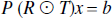
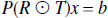
The problem is first formulated in 1 dimension for simplicity. It will be seen that, given a separable point-spread function, the problem generalizes simply to 3 dimensions. The correlation function has been assumed, for simplicity, to be accurately characterized by the PSF, but any separable correlation function can be modeled in this framework. Let P be an n × n matrix, where n is the number of pixels, whose operation on a vector corresponds to the blurring introduced by the PSF. For a symmetric spatially invariant PSF this is a symmetric Toeplitz matrix, although other more general PSF distributions can be accommodated. Let R be an n × r matrix defining r anatomical regions (R ε [0, 1]). Let T be an n × t matrix denoting the t different tissue classifications (T ε [0, 1]). Let b be an n × 1 vector containing the measured tracer concentration. Consequently x is an rt × 1 vector denoting the true radioactivity concentrations in the different classified regions. As constructed, P accounts for the point-spread effect, R ⊙ T account for the tissue-fraction effect, where ⊙ is the Khatri-Rao row product (see Appendix B). The tracer concentration is assumed to be homogeneous within each classified region. A simple example is presented in Fig. 1A, which illustrates how the measured tracer concentrations may be an under- or over-estimation of the true concentration.

FIG. 1.

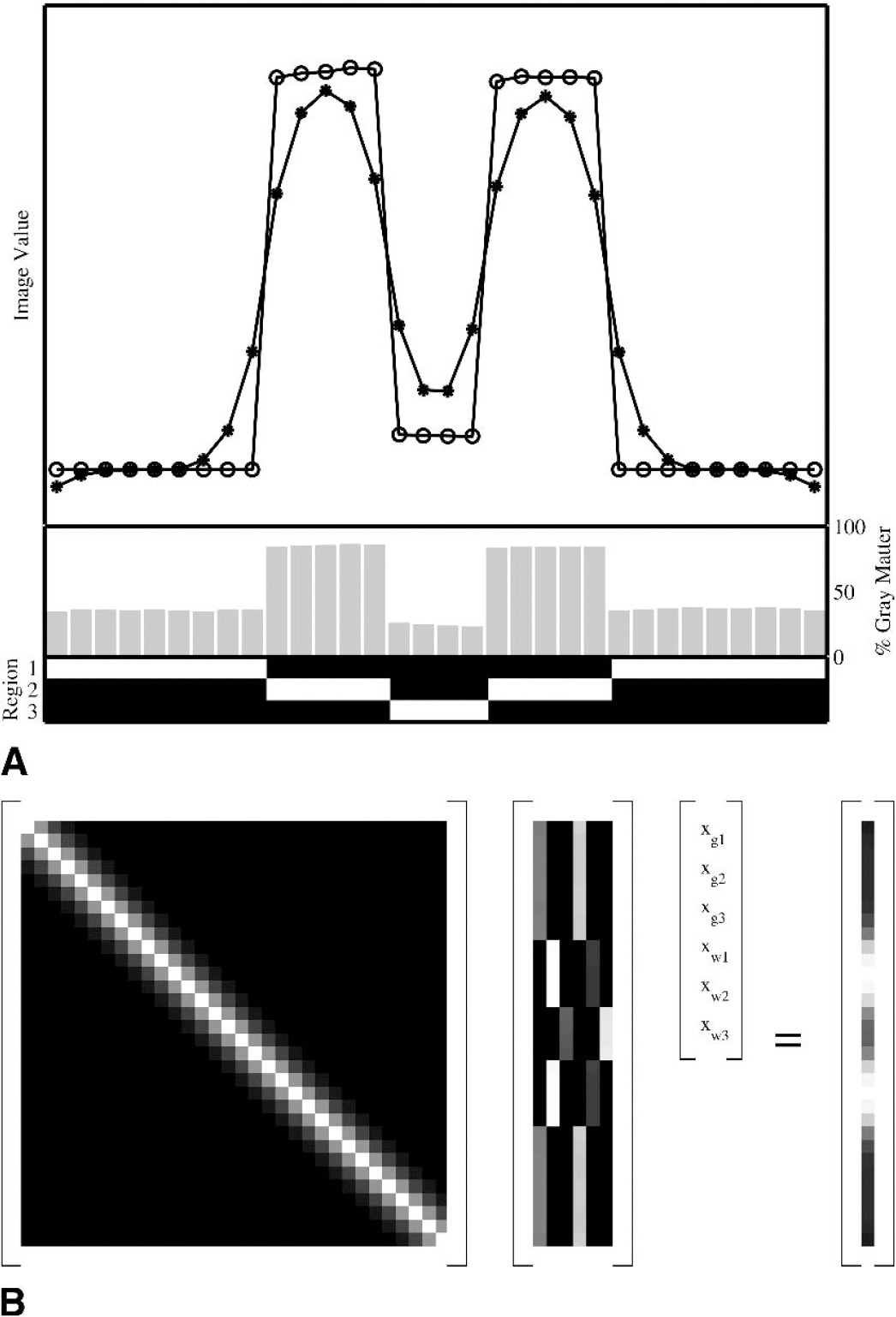
One-dimensional partial volume correction example:(A) (top) tissue radioactivity with (*) and without (o) application of point-spread function;(middle) tissue classification (grey and white only);(bottom) region definitions; and (B) matrix construction of the recovery problem, where x_gi and x_wi are the recovered grey and white matter values, respectively, for region i.

The partial volume problem can then be constructed as a matrix equation, (Fig. 1B),

P (R ⊙ T) x = b

(1)

and the introduction of noise components gives,

P ((R ⊙ T) x + η_{c}) = b + η_{u}

(2)

where η_c and η_u are correlated and uncorrelated noise vectors respectively (see Noise Models). This equation can be rearranged in terms of the recovered signal and noise components1,

(R ⊙ T) x = P^{- 1} b + (P^{- 1} η_{u} + η_{c})

(3)

and is a linear equation of the form Ax =b + ɛ.

The weighted linear least squares solution, x, is determined by minimizing the objective function,

min_{x} {(W^{\frac{1}{2}} ((R ⊙ T) x - P^{- 1} b))}^{T} (W^{\frac{1}{2}} ((R ⊙ T) x - P^{- 1} b))

(4)

where the weighting matrix W is the inverse of the covariance matrix and the solution is given by,

\hat{x} = {({(R ⊙ T)}^{T} W (R ⊙ T))}^{- 1} {(R ⊙ T)}^{T} W P^{- 1} b

(5)

It follows that the variance on the estimates is given by,

\begin{array}{l} v a r (\hat{x}) & = & {({(R ⊙ T)}^{T} W (R ⊙ T))}^{- 1} {((R ⊙ T) x - P^{- 1} b)}^{T} \\ W ((R ⊙ T) x - P^{- 1} b) {(n - r t)}^{- 1} \end{array}

(6)

and the sum of squares accounted for by each ROI is given by,

\begin{array}{l} S S Q_{R O I} & = & {((R ⊙ T) x - P^{- 1} b)}^{T} W^{\frac{1}{2}} Λ (R_{R O I}) \\ W^{\frac{1}{2}} ((R ⊙ T) x - P^{- 1} b) \end{array}

(7)

where Λ() is the diagonal matrix operator, and ROI is the index of the region to be tested.

The preceding equations are all theoretically consistent, and in practice can be used to evaluate partial volume effects. It is interesting to note, however, that the equations only hold true when R ⊙T is a full rank matrix. This might occur (theoretically), for example, if the grey and white composition was constant in a given region. However, because the grey and white classification is probabilistic, and the regions sizes are greater than a few voxels, this is not a problem in practice.

The recovered values for the regionally classified tissues may be estimated once an appropriate noise model has been selected (Eq. 5). The noise model determines the form of the weighting matrix W. It should be noted here that it is of increasing importance that the noise model is estimated correctly to ensure accurate estimates of the parameters above. Hence the accuracy of the weighting is of limited importance for the estimate of tracer concentration (Eq. 5 and Fig. 2). This results in good estimates from both Labbé and Rousset's methods. However, it is more important for estimation of the error on this value (Eq. 6 and Fig. 2) and of vital importance for hypothesis testing of homogeneity derived from the residual sum of squares (Eq. 7).

FIG. 2.

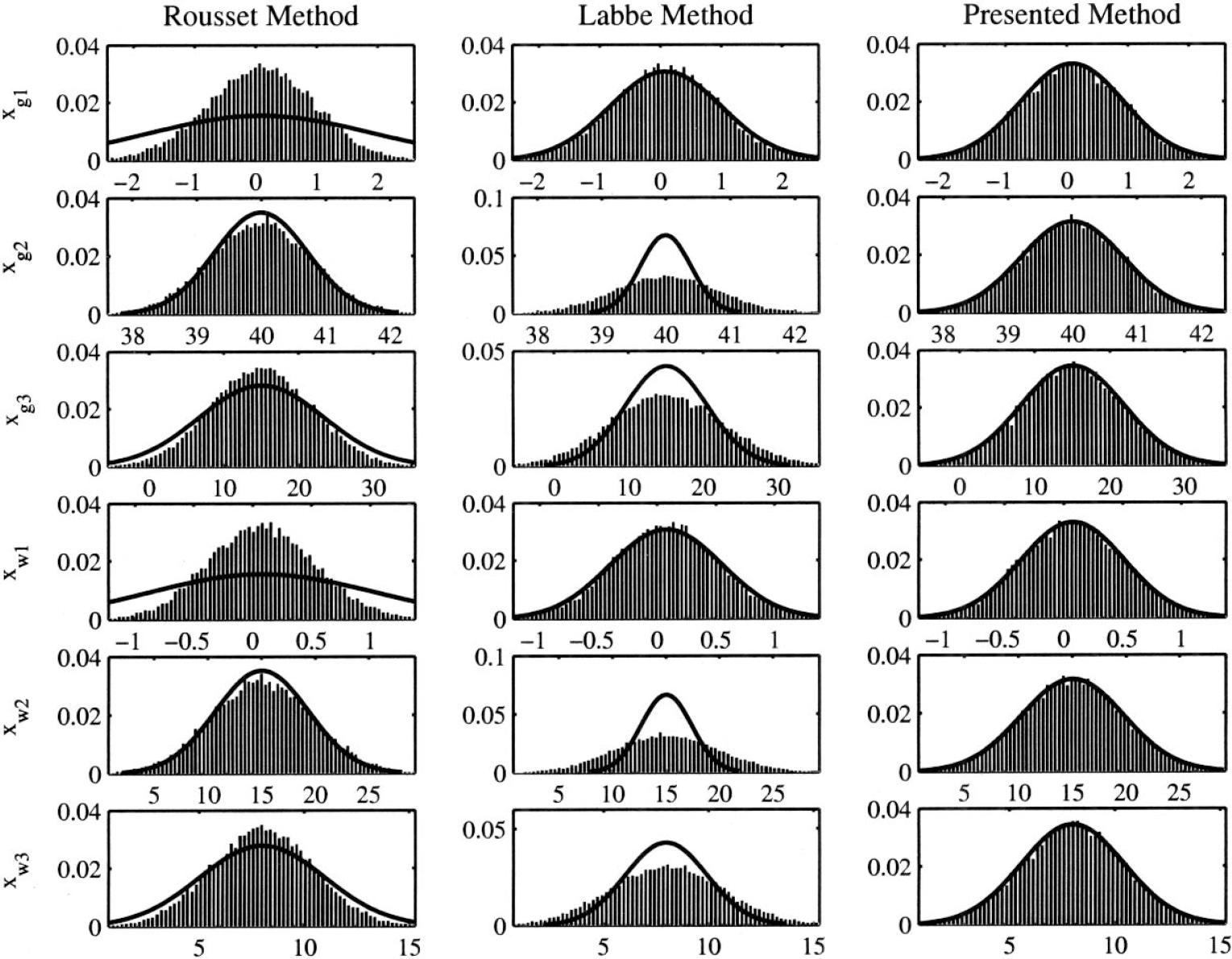
One-dimensional partial volume correction example: noise distribution. Data is simulated using a heterogeneous correlated and homogeneous uncorrelated noise model. The presented method uses this noise structure, whereas the methods of Labbe and Rousset have implicit assumptions about the noise. This figure is intended as a graphical representation of the performance of the differing methods in differing noise situations. Histogram, estimated values; solid line, expected theoretical parameter distribution; x-axis, estimated parameter values; y-axis, probability.

Uncorrelated noise: (η_u ∼ N(0, σ²_u I) and η_c = 0).

If the noise on the measured image is characterized purely by independent identically distributed Gaussian processes with zero mean and standard deviation (SD) σ_u, then the weighting matrix is given by,

W = P^{T} P

(8)

and the weighted least squares solution is,

\hat{x} = {({(R ⊙ T)}^{T} P^{T} P (R ⊙ T))}^{- 1} {(R ⊙ T)}^{T} P^{T} b

(9)

Pure correlated noise: (η_c ∼N (0, D) and η_u = 0).

If the noise post reconstruction has no uncorrelated component then

W = D^{- 1}

(10)

where D is a diagonal matrix representing variances at each pixel (can be homogeneous or inhomogeneous).

The weighted least squares solution is

\hat{x} = {({(R ⊙ T)}^{T} D^{- 1} (R ⊙ T))}^{- 1} {(R ⊙ T)}^{T} D^{- 1} P^{- 1} b

(11)

Correlated noise: (η_c ∼N (0, D) and η_u ∼N (0, σ²_u I)).

If the noise on the image is characterized by both independent identically distributed Gaussian processes then the weighting matrix is given by,

W = {(D + σ_{u}^{2} P^{- 1} {(P^{- 1})}^{T})}^{- 1}

(12)

and the weighted least squares solution is,

\begin{array}{l} \hat{x} & = & {({(R ⊙ T)}^{T} {(D + σ_{u}^{2} P^{- 1} {(P^{- 1})}^{T})}^{- 1} (R ⊙ T))}^{- 1} \\ {(R ⊙ T)}^{T} {(D + σ_{u}^{2} P^{- 1} {(P^{- 1})}^{T})}^{- 1} P^{- 1} b \end{array}

(13)

If any part of the noise structure is signal dependent, then the recovered signal needs to be known. These equations assume that the value for this signal is known. As this will not be the case in heterogeneous signal-dependent noise such as Poisson noise, the solution requires an iterative solution using updates of the estimates, known as Fisher Scoring (McCullagh and Nelder, 1989). This is easily incorporated into the algorithms described.

Methods of Labbé and Rousset

The methods of both Labbé (Labbé et al., 1996) and Rousset (Rousset et al., 1998) and their solutions to the general partial volume correction problem,

P (R ⊙ T) x = b

(14)

can be characterized by their implicit weighting matrices, W, in the weighted least squares framework (Eqs. 4 and 5).

Rousset's method.

The solution given by Rousset is,

x = {({(R ⊙ T)}^{T} P (R ⊙ T))}^{- 1} {(R ⊙ T)}^{T} b

(15)

which is equivalent to a weighted least squares solution in which,

W = P

(16)

Labbé's method.

The solution given by Labbé is

x = {({(R ⊙ T)}^{T} P^{T} P (R ⊙ T))}^{- 1} {(R ⊙ T)}^{T} P^{T} b

(17)

which is equivalent to a weighted least squares solution in which,

W = P^{T} P

(18)

and can be interpreted as the ordinary least squares solution to the problem.

1-dimensional simulations

The 1-D simulations presented here are primarily to demonstrate the problems that can occur if the wrong noise model is assumed when fitting the data, in terms of the estimation of the mean and variance. Although the noise model here is a proportional model, where the noise is proportional to the signal, the underlying problems will also be evident with other noise models.

Simulations were carried out using the example signal representation previously mentioned. This was done so that there would be regions where the signal was both over and under estimated. Noise was added that had both a homogeneous uncorrelated component and a heterogeneous (proportional to the signal) correlated component. The data sets were then simulated with 25,000 repetitions to build up accurate distributions from each of the estimators.

As can be seen in Fig. 2, if the noise model is incorrect, the estimates of the variance of the signal estimate are not correct. The histograms represent the true distribution of the estimate of the value, whereas the solid lines represent the estimated distribution. As can be seen, the variance of true distributions are either under- or over-estimated by the Rousset and Labbé algorithms, and different regions have different over/under estimation. This is owing to the implicit assumptions of the model. The Labbé algorithm assumes uncorrelated noise, and as such the background as the largest region dominates this noise, resulting in a good estimate of the background noise but underestimation in regions of higher noise. The Rousset algorithm has the assumption that the noise is inversely correlated from smoothing, and as such over-estimates the variance in regions with low noise and under-estimates the variance in regions with higher noise. However, the estimates of the signal itself are unbiased for the differing estimators.

Generalization to 3 dimensions

The aforementioned theory has been presented in terms of the 1-D case. A consideration of the assumptions that allows the theory to be generalized to 3 dimensions follows. The only assumption to allow the full generalization of the preceding theory is that each dimension is separable from all the other dimensions. This means that the PSF operator may be applied independently in the x, y, and z dimensions. This assumption is weaker than the assumptions that are made in some previous methods where stationarity was also assumed to facilitate computation (Labbé et al., 1996). However, this assumption was partially removed in later work (Labbé et al., 1998).

It is important to consider other computational aspects that allow for the higher dimension generalization. It is straightforward to see how the computation is handled in the 1-D case with simple matrix and vector operations. The 3-D equivalent is simplified by considering tensor2 operations with restrictive separable properties. Such a construction leads to a computationally efficient algorithm for the implementation of 3-D partial volume correction (see Appendix A).

MATERIALS AND METHODS

The aforementioned theory and algorithms were applied to several data sets for the purpose of validation. Both simulated and measured data were used, primarily with the same specifications, except that, in the simulated data sets, the noise characteristics were known perfectly, whereas, in the measured data sets, the noise characteristics were assumed to be fully characterized.

Simulated data sets

Two simulated data sets were considered. The first consisted of a set of four syringes of differing diameters and considers merely the point-spread effect and required only the definition of R. The second is a flumazenil brain phantom that considered both the point-spread and the tissue-fraction effects and required the definition of both R and T. The simulated data sets were primarily specified using the corresponding measured data sets. The noise variances were determined approximately from the measured data, and then the linear model to be solved was constructed to produce simulated realizations with the exact noise characteristics for the weighting matrix.

Syringe phantom.

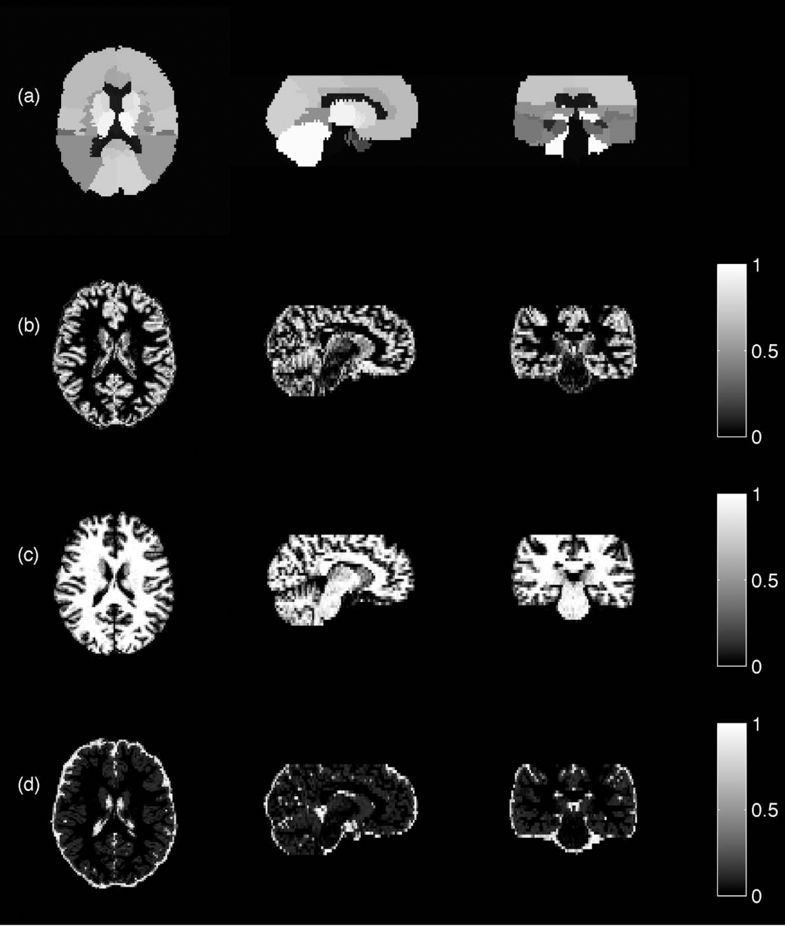
The syringe phantom data were simulated realizations of the measured data obtained from the ECAT ART scanner. The reported PSF characteristics (Bailey et al., 1997) for the ART scanner were used to specify the PSF as a Gaussian kernel, both in the construction of the data set and the subsequent fitting procedures of the algorithms. This allowed for perfect specification of the PSF. The syringe ROIs were generated as cylinders corresponding to the size and location of their counterparts in the physical phantom (Fig. 3). The syringes were simulated to contain 75 kBq/mL of activity at the start of the first acquisition. Noise was added to the images to approximate the measured data for different epochs in time, each epoch being separated by a tracer half-life (in this case 20 minutes for carbon 11). This generated data with a progressively decreasing signal-to-noise ratio. Homogeneous correlated noise was introduced before applying the PSF and subsequently uncorrelated noise was added. The variance of the noise was based on the background noise in the actual measured images at the times of acquisition. Analysis was performed on nondecay corrected data, whereas the results were decay-corrected for ease of comparison. The analysis was carried out using the presented algorithms, as well as Labbé and Rousset's algorithms, to recover the signal and the error estimates. The simulations were also used to assess the possibility of homogeneity testing in well-defined noise models. This was assessed using both the entire data set and a single-syringe ROI, and it was determined whether the expected distribution was obtained by using the Krylov approximation model (see Appendix A).

FIG. 3.

Definition of the 5 regions (including background) for the syringe data set represented by different grey levels (corresponding to R).

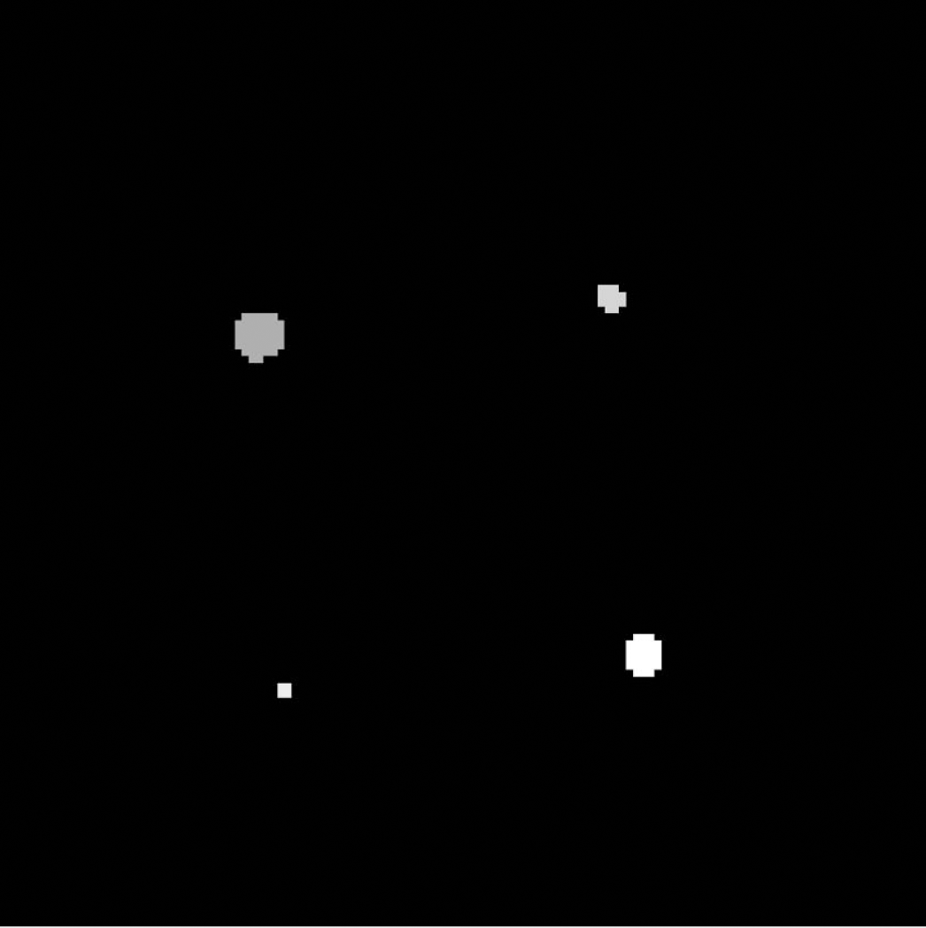
Flumazenil phantom via magnetic resonance imaging segmentation.

The flumazenil simulation was generated using the measured flumazenil data set analyzed below. The data was simulated using the region definitions (R) combined with the tissue classifications (T) (Fig. 4). The simulated V_D values were taken from the measured results. It was then smoothed with the assumed PSF. The noise added was also taken from the noise estimate of the real data. The presented analysis was again used, in a similar way to the syringe data. The estimated noise characteristics of the real model were used to describe the noise in the simulations. The Krylov inhomogeneity testing requires a known variance, and in this case, where the variance is estimated, its use is not applicable.

FIG. 4.

Flumazenil data set:(A) definition of the 43 regions for the flumazenil data set, represented by different grey levels (corresponding to R);(B) grey, (C) white, and (D) CSF tissue classification probabilities (corresponding to T).

Measured data sets

Syringe phantom.

Four syringes of inner diameters 14.8 ± 0.1 mm, 11.9 ± 0.1 mm, 8.6 ± 0.1 mm, and 4.7 ± 0.1 mm were filled with a carbon 11 solution (75 kBq/mL at the start of the first acquisition) and inserted into a 20-cm diameter, 30-cm long cylinder filled with water. The phantom was scanned in an ECAT ART tomograph (CTI/Siemens, Knoxville, TN, U.S.A.) for 10 seconds and 120 seconds, four times, one half-life (20 minutes) apart each time (Fig. 5). The images were reconstructed using the reprojection algorithm (Kinahan and Rogers, 1989) with the ramp and Colscher filters set at Nyquist cut-off frequency. A calculated attenuation correction and a model-based scatter correction (Watson et al., 1996) were applied to the data during reconstruction. The reconstructed images consisted of 47 planes (of which only the center 7 were used in the analysis) having a transaxial spatial resolution of 6.7 mm (at 5 cm from the center of the field of view, where the syringes were located) and an axial spatial resolution of 6.8 mm (FWHM) (Bailey et al., 1997). The presented analysis was again used to calculate the recovery and errors and compared with the methods of Labbé and of Rousset. To assess whether the specified noise model was accurate, the Krylov algorithms were applied to the measured data. This was again done on the both the entire data set and the single syringe, as in the aforementioned simulations.

FIG. 5.

Measured syringe data:(top) 10-second acquisitions (one half-life apart);(bottom) 120-second acquisitions (one half-life apart).

Measured flumazenil.

A [¹¹C]flumazenil data set was obtained from an ongoing clinical study and acquired according to a protocol described previously (Koepp et al., 1996;Richardson et al., 1996). Briefly, the scan was performed in 3-D mode on a 953 B Siemens/CTI PET camera with a reconstructed image resolution of approximately 4.8×4.8×5.2 mm at FWHM (Bailey, 1992) for 31 simultaneously acquired planes with reconstructed voxel sizes of 2.09×2.09×3.42 mm. A convolution subtraction method was used to correct for scatter (Bailey and Meikle, 1994) and axial scaling with the inverse of the scanner's axial profile was applied to obtain uniform efficiency throughout the field of view (Grootoonk, 1995). Voxel-by-voxel parametric images of [¹¹C]flumazenil volume of distribution (V_D) were then produced from the brain uptake and arterial metabolite-corrected plasma input functions using a single compartmental tracer kinetic model and estimates of the variance of the parameters calculated (Aston et al., 2000) and is shown in Fig. 6. A region template containing 43 regions was used, which was derived from the MRI of a single brain (Holmes et al., 1998) that has been widely used as a reference brain. To subdivide the flumazenil data set, the region template was spatially warped to fit the subject's MRI data set. This was performed using linear and nonlinear transformations (Ashburner and Friston, 1999) with parameters derived from the MRI data set associated with the template (Hammers et al., in press) The subject's own MRI was also segmented (Lemieux et al., 1999) into grey matter, white matter, and CSF. The transformed region template and the MRI data sets were then coregistered with the PET data set (Ashburner and Friston, 1997). PVC to recover the corrected V_D values was applied, using weights derived from the variance map calculated as part of the analysis. Again, the Krylov method was not appropriate for this data set, owing to its unknown variance.

FIG. 6.

Flumazenil:(A) volume of distribution;(B) volume of distribution error (both prior to correction).

All data analysis was performed in Matlab (Mathworks Inc., Natick, MA, U.S.A.) running on a 650 MHz Pentium PC.

RESULTS

In all the studies it was found that the purely correlated noise algorithms were unstable in the presence of uncorrelated noise in the data. This is owing to the ill-conditioned nature of the inverse of the correlation matrix. Because all the data were assumed to have a true noise structure that included a component of uncorrelated noise, the results of purely correlated algorithms have been omitted because of their instability. This result was not unexpected, and in practice purely correlated noise algorithms are seldom if ever used to analyze data.

Simulated data sets

Syringe phantom.

The syringe simulations showed that good recovery of the true signal was achieved with all algorithms (Table 1), at different times, with earlier frames, where there are more counts, yielding closer to truth estimates than later frames (all frames are decay corrected back to the start). However, the estimates of the SD in the Labbé and Rousset algorithms were too low, which would lead to the rejection of null hypotheses with the true mean in some cases. This did not occur with the presented algorithm.

TABLE 1.

Results from partial volume correction of simulated syringe data from Rousset, Labbé and presented methods

			Syringe diameter (mm)
	Time (sec)		14.8			11.9			8.6			4.7			Bgd
Method	Start	Dur	NC	x̂	sd(x̂)	NC	x̂	sd(x̂)	NC	x̂	sd(x̂)	NC	x̂	sd(x̂)	NC	x̂	sd(x̂)
Roussett	0	10	52.4	74.8	0.17	48.6	76.4	0.22	36.8	73.4	0.35	17.9	68.6	0.87	0.12	−0.023	0.007
Labbe	0	10	52.4	74.7	0.27	48.6	76.5	0.37	36.8	73.5	0.62	17.9	71.1	1.73	0.12	−0.023	0.011
Presented	0	10	52.4	74.8	0.77	48.6	76.3	0.98	36.8	73.1	1.47	17.9	69.7	3.48	0.12	−0.023	0.035
Rousset	10	120	52.7	75.1	0.09	48.0	75.4	0.12	37.9	75.5	0.20	19.5	74.5	0.49	0.15	0.010	0.004
Labbe	10	120	52.7	75.2	0.08	48.0	75.4	0.11	37.9	75.6	0.19	19.5	73.5	0.51	0.15	0.010	0.003
Presented	10	120	52.7	75.1	0.23	48.0	75.4	0.29	37.9	75.3	0.44	19.5	74.4	1.04	0.15	0.011	0.010
Rousset	1,200	10	51.3	73.2	0.23	46.8	73.6	0.29	39.4	78.7	0.47	22.4	85.9	1.17	0.09	−0.052	0.009
Labbe	1,200	10	51.3	73.1	0.39	46.8	73.5	0.53	39.4	79.9	0.89	22.4	83.9	2.47	0.09	−0.057	0.015
Presented	1,200	10	51.3	73.2	1.11	46.8	73.6	1.40	39.4	78.3	2.10	22.4	86.1	4.98	0.09	−0.046	0.050
Rousset	1,210	120	52.6	75.0	0.10	48.1	75.5	0.13	37.7	75.2	0.21	19.5	74.7	0.53	0.16	0.020	0.004
Labbe	1,210	120	52.6	74.9	0.11	48.1	75.5	0.15	37.7	75.2	0.25	19.5	73.9	0.71	0.16	0.021	0.004
Presented	1,210	120	52.6	75.1	0.32	48.1	75.5	0.40	37.7	75.2	0.60	19.5	74.7	1.42	0.16	0.020	0.014
Rousset	2,400	10	53.0	75.5	0.31	49.1	77.1	0.40	40.5	80.7	0.64	20.3	77.6	1.60	0.23	0.085	0.013
Labbe	2,400	10	53.0	75.5	0.55	49.1	77.2	0.74	40.5	80.6	1.25	20.3	75.0	3.47	0.23	0.084	0.021
Presented	2,400	10	53.0	75.1	1.55	49.1	77.4	1.96	40.5	80.8	2.94	20.3	79.6	6.96	0.23	0.087	0.071
Rousset	2,410	120	52.2	74.4	0.12	47.0	73.9	0.15	38.0	75.7	0.24	19.5	74.8	0.61	0.09	−0.052	0.005
Labbe	2,410	120	52.2	74.3	0.16	47.0	73.8	0.21	38.0	75.5	0.36	19.5	76.2	0.99	0.09	−0.053	0.006
Presented	2,410	120	52.2	74.5	0.44	47.0	74.1	0.56	38.0	75.8	0.84	19.5	75.3	2.00	0.09	−0.052	0.020
Rousset	3,600	10	51.9	74.0	0.42	47.9	75.2	0.55	36.5	72.8	0.88	17.0	65.2	2.19	0.14	0.004	0.018
Labbe	3,600	10	51.9	74.2	0.77	47.9	74.0	1.04	36.5	70.9	1.76	17.0	63.7	4.88	0.14	0.004	0.030
Presented	3,600	10	51.9	74.0	2.18	47.9	75.8	2.76	36.5	73.7	4.14	17.0	65.4	9.82	0.14	0.007	0.099
Rousset	3,610	120	52.7	75.2	0.14	47.4	74.5	0.19	38.0	75.8	0.30	18.9	72.4	0.75	0.16	0.020	0.006
Labbe	3,610	120	52.7	75.4	0.22	47.4	74.5	0.29	38.0	75.5	0.50	18.9	73.8	1.38	0.16	0.020	0.008
Presented	3,610	120	52.7	75.0	0.62	47.4	74.4	0.78	38.0	75.8	1.17	18.9	71.9	2.78	0.16	0.020	0.028

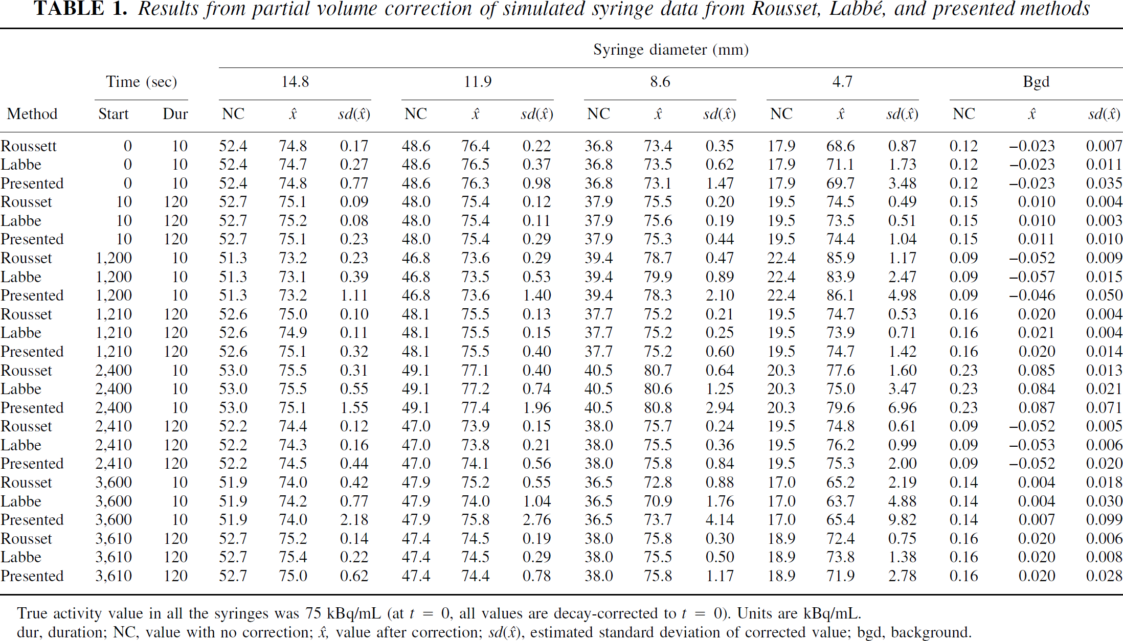
True activity value in all the syringes was 75 kBq/mL (at t = 0, all values are decay-corrected to t = 0). Units are kBq/mL.

dur, duration; NC, value with no correction; x̂, value after correction; sd(◯), estimated standard deviation of corrected value; dur, duration; bgd, background.

The recovery rates of the different algorithms, defined as the percentage recovery of the true value, are shown in Fig. 7. As can be seen, all the algorithms recover the signal well, even as the size of the syringe dereases. However, the recovery becomes worse as the signal-to-noise ratio decreases, equivalent to later frames in the scan.

FIG. 7.

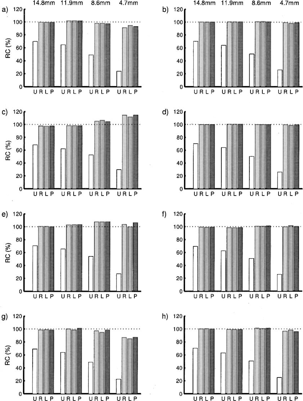
Recovery rates from the simulated syringe data. The graphs (A—H) represent the different start times and acquisition lengths in temporal order, with the first column (A, C, E, G) showing the short 10-second acquisitions, and the second column (B, D, F, H) the longer 120-second acquisitions. The measurements above the graph refer to the syringe sizes. U, the uncorrected data; R, Rousset's method; L, Labbé's method; P, the presented method.

The presented algorithm took approximately 10 minutes per frame to run. This is dependent on the noise model, as can be seen in equation A.8 in the Appendix. The condition number of the matrices in the equations depends on the relative contributions of the noise. The Labbé and Rousset algorithms took approximately 10 seconds per frame to run.

Whereas the overall sum of squares (SSQ) for the entire data set was consistent with the noise model, the Krylov subspace approximation was not able to accurately distinguish between the different regional SSQs for a small number of iterations. In principle, however, with a large enough amount of memory the algorithm would become increasingly more accurate. The Krylov subspace algorithms gave a good approximation to the SSQ for a single ROI. As the number of iterations was increased, so was the accuracy of the approximation (Fig. 8). However, the increase in the number of iterations also required an increase in memory, and so would not allow the approximation to necessarily be used in practice on larger data sets.

FIG. 8.

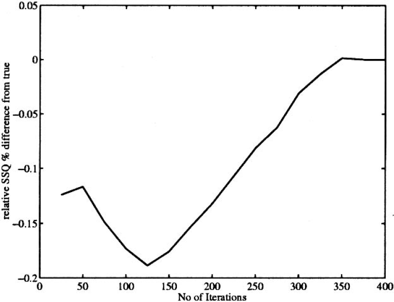
Typical Krylov iterations for simulated syringe.

Flumazenil phantom via magnetic resonance imaging segmentation.

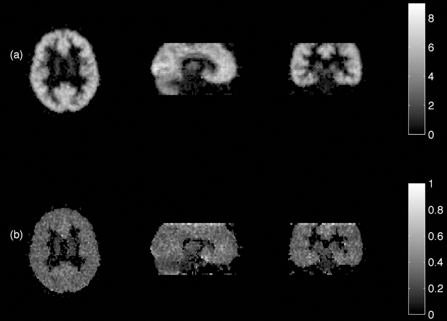
The recovered image from the simulation is shown in Fig. 9. There was a good correlation between the recovered values and the simulated values (R = 0.98) in the grey and white regions (Table 2), although CSF regions were not well recovered. This is owing to the low probability of the CSF in some regions and the consequent difficulty in estimation. The actual values for the CSF, however, are not usually of interest, but it is important to include them in the model.

TABLE 2.

Results from simulated [¹¹C]flumazenil data set: grey matter and white matter volume-of-distribution values recovered by partial volume correction for a representative set of anatomical regions and compared with the precorrection results

	Grey matter			White matter
Region	True	Rec	Sd	True	Rec	Sd
Amygdala
R	7.21	5.32	0.35	0.48	1.25	0.33
L	5.83	4.28	0.35	0.37	0.65	0.27
Middle inferior temporal gyrus
R	8.32	7.70	0.17	1.80	1.94	0.03
L	10.83	10.86	0.08	2.49	2.67	0.03
Frontal lobe
R	9.23	9.03	0.03	2.31	2.45	0.01
L	8.81	8.63	0.03	2.96	3.14	0.01
Parietal lobe
R	10.38	10.25	0.04	1.81	2.02	0.01
L	10.51	10.53	0.04	2.02	2.25	0.01
Occipital lobe
R	7.51	7.36	0.06	4.19	4.31	0.02
L	6.73	6.53	0.06	4.46	4.64	0.02
Thalamus
R	4.76	5.09	0.18	1.81	1.88	0.03
L	5.32	5.21	0.16	1.10	1.20	0.03
Cerebellum
R	6.26	6.24	0.03	2.31	2.44	0.01
L	6.61	6.54	0.03	2.12	2.25	0.01

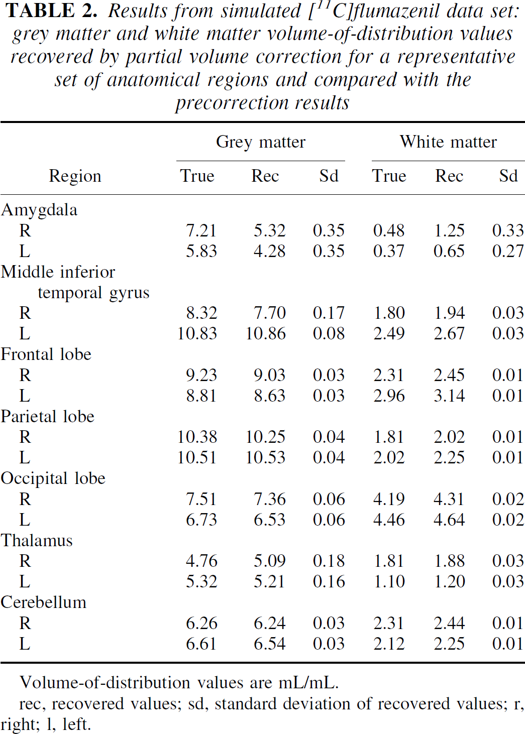
Volume-of-distribution values are mL/mL.

rec, recovered values; sd, standard deviation of recovered values; r, right; l, left.

FIG. 9.

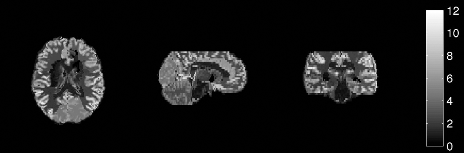
Simulated flumazenil data projected onto magnetic resonance imaging template.

The algorithms speed is related directly to the number of regions and tissue classifications defined (rt). The time increases linearly (assuming the algorithm does not have to be split for memory purposes), with an addiion of approximately 10 to 15 seconds per extra classified region.

Measured data sets

Syringe phantom.

As can be seen (Table 3), the measured data sets were less well modeled by the noise characteristics than was the simulated data. This is not unexpected, because the simulated data had perfect noise specification. However, the new method gives apparently more plausible estimates for the error of the estimate, given the true value, especially in the higher noise frames. Because the rates of recovery are also derived from these values, the rates of recovery are worse than in the simulated case, as can be seen in Fig. 10. However, all algorithms continued to give good recovery of the signal even with the small syringe.

TABLE 3.

Results from partial volume correction of simulated syringe data from Rousset, Labbé and presented methods

			Syringe diameter (mm)
	Time (sec)		14.8			11.9			8.6			4.7			Bgd
Method	Start	Dur	NC	x̂	sd(x̂)	NC	x̂	sd(x̂)	NC	x̂	sd(x̂)	NC	x̂	sd(x̂)	NC	x̂	sd(x̂)
Roussett	0	10	51.4	73.2	0.16	50.5	79.4	0.20	39.7	79.2	0.32	20.1	76.7	0.81	0.19	0.045	0.007
Labbe	0	10	51.4	74.0	0.28	50.5	80.0	0.37	39.7	80.3	0.63	20.1	83.7	1.73	0.19	0.040	0.011
Presented	0	10	51.4	72.7	0.80	50.5	78.2	1.01	39.7	78.5	1.52	20.1	75.1	3.59	0.19	0.049	0.036
Rousset	10	120	52.8	75.3	0.10	50.5	79.3	0.13	39.9	79.4	0.21	19.5	74.7	0.53	0.17	0.023	0.004
Labbe	10	120	52.8	75.7	0.09	50.5	79.8	0.12	39.9	81.0	0.21	19.5	77.6	0.59	0.17	0.019	0.004
Presented	10	120	52.8	74.8	0.24	50.5	78.7	0.30	39.9	78.3	0.46	19.5	73.4	1.08	0.17	0.025	0.011
Rousset	1,200	10	52.8	75.3	0.20	52.5	82.4	0.26	40.9	81.6	0.41	19.9	76.1	1.03	0.20	0.048	0.008
Labbe	1,200	10	52.8	75.3	0.38	52.5	82.9	0.51	40.9	81.7	0.87	19.9	80.2	2.41	0.20	0.047	0.015
Presented	1,200	10	52.8	75.2	1.12	52.5	82.5	1.41	40.9	81.8	2.12	19.9	73.7	5.02	0.20	0.048	0.051
Rousset	1,210	120	52.3	74.6	0.11	50.7	79.7	0.14	39.8	79.3	0.23	20.0	76.6	0.56	0.18	0.037	0.005
Labbe	1,210	120	52.3	75.3	0.12	50.7	80.5	0.16	39.8	80.3	0.28	20.0	78.1	0.77	0.18	0.034	0.005
Presented	1,210	120	52.3	74.0	0.33	50.7	79.1	0.42	39.8	78.4	0.63	20.0	76.7	1.50	0.18	0.040	0.015
Rousset	2,400	10	53.8	76.7	0.26	52.6	82.6	0.34	37.5	74.8	0.55	16.8	64.0	1.37	0.22	0.072	0.011
Labbe	2,400	10	53.8	76.5	0.54	52.6	82.8	0.72	37.5	75.4	1.22	16.8	73.0	3.38	0.22	0.070	0.021
Presented	2,400	10	53.8	77.0	1.56	52.6	81.7	1.97	37.5	74.7	2.96	16.8	62.0	7.02	0.22	0.072	0.071
Rousset	2,410	120	52.8	75.3	0.12	50.8	79.8	0.16	40.1	79.9	0.25	18.8	72.1	0.62	0.18	0.036	0.005
Labbe	2,410	120	52.8	75.8	0.16	50.8	80.5	0.22	40.1	81.0	0.37	18.8	74.7	1.03	0.18	0.033	0.006
Presented	2,410	120	52.8	74.9	0.45	50.8	79.1	0.57	40.1	79.5	0.86	18.8	71.9	2.05	0.18	0.038	0.021
Rousset	3,600	10	56.5	80.5	0.35	50.1	78.7	0.46	35.5	70.8	0.73	16.8	64.1	1.84	0.21	0.064	0.015
Labbe	3,600	10	56.5	80.8	0.75	50.1	80.4	1.00	35.5	74.2	1.70	16.8	72.4	4.71	0.21	0.057	0.029
Presented	3,600	10	56.5	80.3	2.18	50.1	77.2	2.76	35.5	70.0	4.14	16.8	61.9	9.81	0.21	0.067	0.099
Rousset	3,610	120	52.6	74.9	0.14	49.4	77.7	0.18	41.8	83.2	0.29	19.8	75.7	0.71	0.19	0.048	0.006
Labbe	3,610	120	52.6	75.4	0.22	49.4	78.3	0.30	41.8	83.2	0.51	19.8	81.2	1.40	0.19	0.045	0.009
Presented	3,610	120	52.6	74.5	0.64	49.4	77.2	0.80	41.8	83.8	1.21	19.8	74.1	2.86	0.19	0.050	0.029

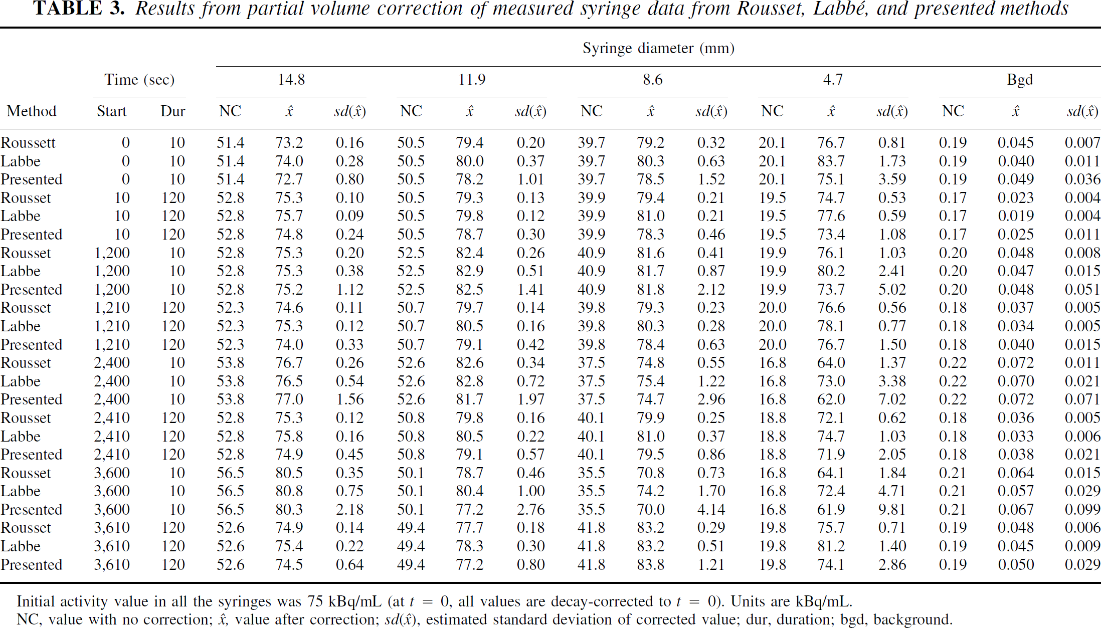
Initial activity value in all the syringes was 75 kBq/mL (at t = 0, all values are decay-corrected to t = 0). Units are kBq/mL.

NC, value with no correction; x̂, value after correction; sd(◯), estimated standard deviation of corrected value; dur, duration; bgd, background.

FIG. 10.

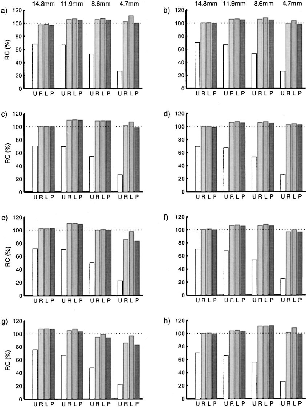
Recovery rates from the measured syringe data. The graphs (A—H) represent the different start times and acquisition lengths in temporal order, with the first column (A, C, E, G) showing the short 10-second acquisitions, and the second column (B, D, F, H) the longer 120-second acquisitions. The measurements above the graph refer to the syringe sizes. U, the uncorrected data; R, Rousset's method; L, Labbé's method; P, the presented method.

As might have been expected, the Krylov algorithm did not allow for hypothesis testing of homogeneity. This was almost certainly owing to inadequate specification of the noise model. The total SSQ was not as expected if the noise model had been correctly specified, and the SSQ of the single syringe was also affected this way. The noise model is of increasing importance, from estimation-of-signal, then errors through to hypothesis testing. In the case of hypothesis testing, the noise model must be assumed to be fully characterized, including a known variance. However, with more accurate specification of the noise model, the possibility of hypothesis testing remains.

Measured flumazenil.

The flumazenil data was well recovered in the measured data (Fig. 11;Table 4), except in the few regions where the grey/white border is less well defined (e.g., occipital lobe), giving the impression that the binding was taking place in the white matter. Again, the CSF was highly variable and, as such, is not included in Table 4.

TABLE 4.

Results from measured [¹¹C]flumazenil data set: grey matter and white matter volume-of-distribution values recovered by partial volume correction for a representative set of anatomical regions and compared with the precorrection results

	Grey matter			White matter
Region	Pre	Rec	Sd	Pre	Rec	Sd
Amygdala
R	3.30	7.21	0.39	2.78	0.48	0.38
L	4.01	5.83	0.40	2.68	0.37	0.31
Middle inferior temporal gyrus
R	5.51	8.32	0.20	3.56	1.80	0.04
L	5.90	10.83	0.09	3.91	2.49	0.04
Frontal lobe
R	5.78	9.23	0.03	3.55	2.31	0.01
L	5.35	8.81	0.03	3.91	2.96	0.01
Parietal lobe
R	5.85	10.38	0.05	2.98	1.81	0.01
L	5.74	10.51	0.05	3.07	2.02	0.02
Occipital lobe
R	5.47	7.51	0.07	4.86	4.19	0.03
L	5.42	6.73	0.06	4.77	4.46	0.03
Thalamus
R	2.10	4.76	0.20	1.55	1.81	0.04
L	3.06	5.32	0.19	1.13	1.10	0.03
Cerebellum
R	4.29	6.26	0.03	2.88	2.31	0.01
L	4.49	6.61	0.03	3.03	2.12	0.01

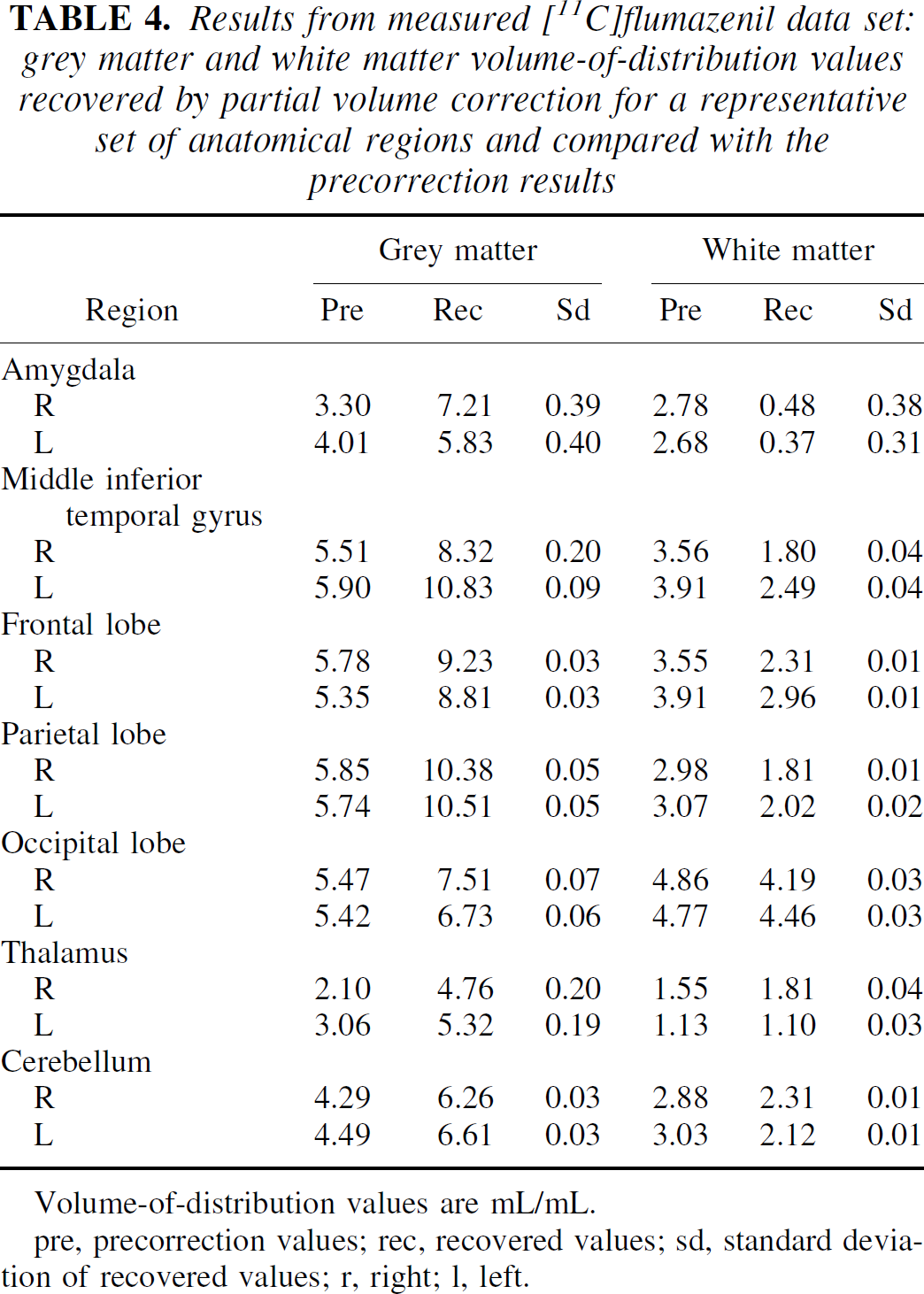
Volume-of-distribution values are mL/mL.

pre, precorrection values; rec, recovered values; sd, standard deviation of recovered values; r, right; l, left.

FIG. 11.

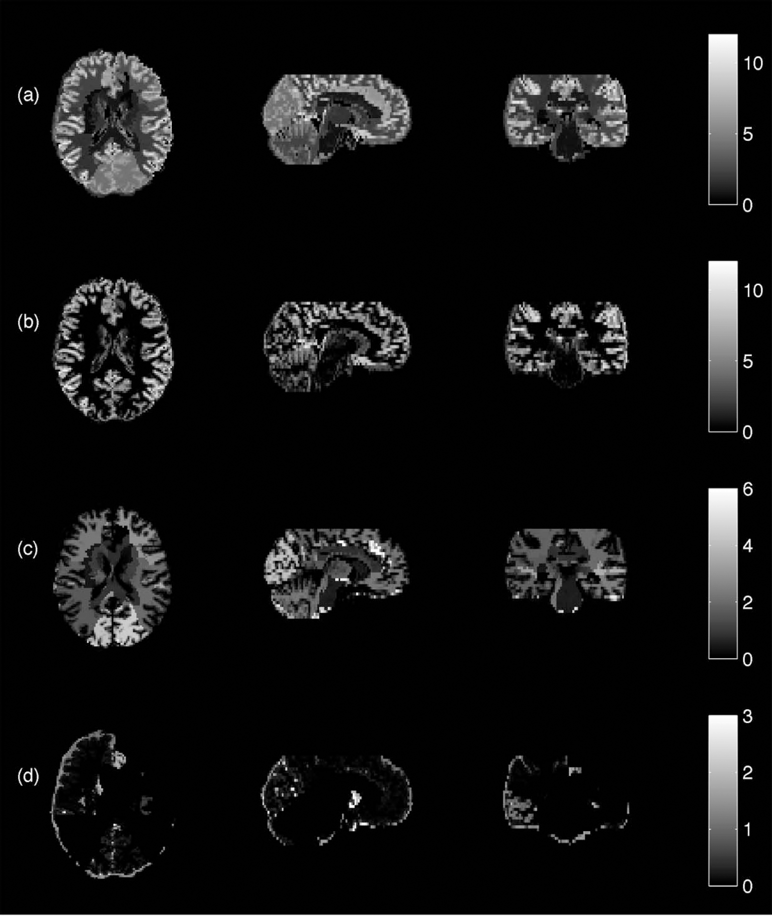
Measured flumazenil data projected onto segmented magnetic resonance imaging template after partial volume correction:(A) total, (B) grey matter, (C) white matter, (D) CSF.

DISCUSSION

The purpose of the present work was first, to bring together previous approaches to the PVC problem into a coherent mathematical framework; second, to devise rapid computational algorithms based on explicit definitions of noise models; and third, to explore the possibilities of obtaining further information on the associated errors and questions about the homogeneity of the defined ROIs.

In the present paper partial volume effect models have been formulated in terms of linear matrix equations, in which the observed image is expressed as the product of the true concentration in a set of regions and matrices accounting for tissue-fraction and point-spread effects. The true local concentration is then estimated by the appropriate weighted least squares procedure. It is shown that the choice of algorithm for obtaining the least squares solution is dependent on the assumed noise models. Three noise models were considered: noise correlated by the PSF, uncorrelated noise, and a combination of both. Previous presentations of this problem in the literature have been principally concerned with algorithms for obtaining solutions, but as a consequence have implicit assumptions about the noise model. The computational schemes presented here incorporate explicit assumptions. They differ with respect to ease of computation and inherent stability in the face of misspecification of the noise model.

Three aspects of the solution have been considered. The first aspect is obtaining an estimate of the mean regional radioactivity. It is shown that mean regional radioactivity estimate is relatively insensitive to the noise models in routine use. The principal assumption associated with this aspect of the solution is the homogeneity of the ROIs and the correct classification of the tissue type within those ROIs. Rapid algorithms are presented here, which enable partial volume corrected estimates to be readily calculated. The second aspect is obtaining an estimate of the variance of the estimates; as would be expected, this is more dependent on the assumption of a correct noise model. The third aspect considered is the ability to test the assumed homogeneity of the ROIs. The Krylov method developed allows for hypothesis testing of inhomogeneity. However, in practice this is limited by two factors: first, as the volumes and number of tissues increase the memory required for the computations becomes too large on a standard desktop PC; and second, that the approximation of the noise model for measured data is not sufficiently accurate.

In the simulations, realizations with noise of a completely characterized structure were presented, and it was shown that this resulted in good recovery of both the parameter estimates and the errors associated with them. However, in practice it is well known that the noise structure will not be perfectly characterized. It was seen in the true syringe phantom experiments that, while this leads to estimates with greater variability than might be expected from the simulations, the estimates themselves remain stable. The variability, although increased, is still a more accurate estimate of the variability than using error estimates derived from the models of either Rousset or Labbé. It was seen that the estimates are only as good as the underlying tissue data, and this was especially evident in the occipital cortex of the flumazenil study. In the occipital cortex the grey matter/white matter boundary is less well defined than in other regions, and this leads to the estimates of the activity from the grey and white matter areas being difficult to distinguish. This is a problem in all techniques that use structural definition, especially when the structure cannot be well defined.

The nature of partial volume effects means that, even if an accurate estimation technique is specified and validated against phantom models, the underlying assumptions of tissue homogeneity and the point-spread effect are critical. In performing partial volume correction using MRI imaging, partial volume corrections are being based on information that is itself subject to partial volume effects, albeit on a much smaller scale. True direct validation requires estimation and the recovery of tissue values from sources where these tissue values can also be directly measured outside the PET system. This is also true of validation of MRI segmentation techniques. Only a minority of partial volume techniques have considered this highly complex methodologic problem (Iida et al., 2000), and this was not the focus of the work presented here. However, if models for the errors from this source were available, these could possibly be incorporated into the method presented.

The characterization of the PSF is of central importance. The matrix formulation allows complex nonstationary characterization. However, it is important to note that the algorithms presented here require that the PSF is separable (i.e., it can be applied independently in the x, y and z directions). The separability of the PSF was exploited in devising computationally fast algorithms. The dependence of the final estimates on the accuracy of the PSF characterization has not been considered here, but would be dependent on ROI shape, noise in the image, tissue classification, shape of the PSF and relative FWHM, and would need testing for individual applications. Similarly, we have not considered the effects of image misregistration, tissue misclassification (Meltzer et al., 1999;Reilhac et al., 2001), or ROI misplacement. Ideally, these could be tested for in terms of inhomogeneity. The principal problem associated with this, however, is inadequate characterization of the noise model as discussed previously. Accurate characterization of the noise model in image space is difficult, but might be simplified by considering the problem in sinogram space (Carson, 1986). This would, however, offer challenges associated with specification of the model in sinogram space.

Computational schemes appropriate for the various noise models have been presented and are expanded further in the appendix. These schemes can be easily implemented and have proved to be very fast (e.g., the 43-region flumazenil volume with 3 tissue classifications is calculated in approximately 30 minutes on a desktop computer). In principle, they can be applied to raw PET data, or to parametric images derived from application of temporal kinetic models to the raw data. Application to parametric images has the implicit assumption that the kinetic model is linear in the functional parameter. In this case, the noncorrelated model, which requires no estimates of multiplicative noise, is probably sufficient to obtain an estimate of a classified regional activity together with its error.

Strictly, application to nonlinear temporal kinetic modeling should be applied frame by frame. This has the advantages of allowing specification of a more accurate noise model including both correlated and uncorrelated components, as well as producing error estimates that can then be used for weighting in the subsequent kinetic fitting. Estimates of the additive noise component can be obtained from the background. In practice, however, effects of the nonlinearity can be assessed in individual cases, and the simpler, uncorrelated PVC model applied to the parametric image, if the bias is considered acceptable.

Footnotes

1

η_x represents the noise process and hence the sign is unimportant here.

2

Tensors are merely generalizations of vectors (1D) and matrices (2D) in higher dimensions.

Acknowledgments

The authors would like to thank Peter Neelin and Federico Turkheimer for useful discussions, as well as two anonymous referees for their constructive comments.

ALGORITHMS FOR 3-DIMENSIONAL IMPLEMENTATION

GLOSSARY

References

Allen

Baglama

Boyd

(2000) Numerical approximation of the product of the square root of a matrix with a vector. Linear Algebra and Its Applications 310:167–181

Ashburner

Friston

(1997) Multimodal image coregistration and partitioning—a unified framework. Neuroimage 6:209–217

Ashburner

Friston

(1999) Nonlinear spatial normalization using basis functions. Hum Brain Mapp 7:254–266

Asselin

M-C

Cunningham

Turjanski

Wahl

Bloomfield

Gunn

Nahmias

(2001) Venous sinuses vs on-line arterial sampling as input functions in PET. In: Physiological imaging of the brain with PET ( Gjedde

Hansen

Knudsen

Paulson

, eds), San Diego, CA: Academic Press, pp 73–81

Aston

JAD

Gunn

Worsley

Evans

Dagher

(2000) A statistical method for the analysis of positron emission tomography neuroreceptor ligand data. Neuroimage 12:245–256

Axelsson

(1994) Iterative solution methods. New York, NY: Cambridge University Press

Bailey

(1992) 3d acquisition and reconstruction in positron emission tomography. Ann Nucl Med 6:123–130

Bailey

Meikle

(1994) A convolution-subtraction scatter correction method for 3d pet. Phys Med Biol 39:411–424

Bailey

Young

Bloomfield

Meikle

Glass

Myers

Spinks

Watson

Luk

Peters

Jones

(1997) ECAT ART—a continuously rotating PET camera: performance characteristics, initial clinical studies, and installation considerations in a nuclear medicine department. Eur J Nucl Med 24:6–15

10.

Carson

(1986) A maximum likelihood method for region-of-interest evaluation in emission tomography. J Comput Assist Tomogr 10:654–663

11.

Carson

Yan

Daubewitherspoon

Freedman

Bacharach

Herscovitch

(1993) An approximation formula for the variance of PET region-of-interest values. IEEE Trans Med Imaging 12:240–250

12.

Golub

Van Loan

(1983) Matrix computations. Baltimore, MD: Johns Hopkins University Press

13.

Grootoonk

(1995) Dual energy window correction for scattered photons in 3D positron emission tomography [Ph.D. thesis]. Surrey, U.K.: University of Surrey

14.

Hammers

Koepp

Free

Brett

Richardson

Labbé

Cunningham

Brooks

Duncan

(2002) Implementation and application of a new brain template for multiple volumes of interest. Hum Brain Mapp 15:165–174

15.

Hoffman

Huang

Phelps

(1979) Quantitation in positron emission computed tomography. Part I: effect of object size. J Comput Assist Tomogr 3:299–308

16.

Holmes

Hoge

Collins

Woods

Toga

Evans

(1998) Enhancement of mr images using registration for signal averaging. J Comput Assist Tomogr 22:324–333

17.

Iida

Law

Pakkenberg

Krarup-Hansen

Eberl

Holm

Hansen

Gundersen

Thomsen

Svarer

Ring

Friberg

Paulson

(2000) Quantitation of regional cerebral blood flow corrected for partial volume effect using O-15 water and PET. Part I: theory, error analysis, and stereologic comparison. J Cereb Blood Flow Metab 20:1237–1251

18.

Karp

Daube-Witherspoon

Muehllehner

(1991) Factors affecting accuracy and precision in PET volume imaging. J Cereb Blood Flow Metab 11:A38–44

19.

Kinahan

Rogers

(1989) Analytic 3D image-reconstruction using all detected events. IEEE Trans Nucl Sci 36:964–968

20.

Koepp

Richardson

Brooks

Poline

Van Paesschen

Friston

Duncan

(1996) Cerebral benzodiazepine receptors in hippocampal sclerosis: an objective in vivo analysis. Brain 119(Pt 5):1677–1687

21.

Labbé

Froment

Kennedy

Ashburner

Cinotti

(1996) Positron emission tomography metabolic data corrected for cortical atrophy using magnetic resonance imaging. Alzheimer Dis Assoc Disord 10:141–170

22.

Labbé

Koepp

Ashburner

Spinks

Richardson

Duncan

Cunningham

(1998) Absolute PET quantification with correction for partial volume effects within cerebral structures. In: Quantitative functional brain imaging with positron emission tomography ( Carson

Daube-Witherspoon

Herscovitch

, eds), San Diego, CA: Academic Press, pp 59–66

23.

Law

Iida

Holm

Nour

Rostrup

Svarer

Paulson

(2000) Quantitation of regional cerebral blood flow corrected for partial volume effect using 0–15 water and PET. Part II: normal values and gray matter blood flow response to visual activation. J Cereb Blood Flow Metab 20:1252–1263

24.

Leahy

(2000) Statistical approaches in quantitative positron emission tomography. Stat Computing 10:147–165

25.

Lemieux

Hagemann

Krakow

Woermann

(1999) Fast, accurate, and reproducible automatic segmentation of the brain in T1-weighted volume MRI data. Magn Reson Med 42:127–135

26.

Mazziotta

Phelps

Plummer

Kuhl

(1981) Quantitation in positron emission computed tomography. Part V: physical—anatomical effects. J Comput Assist Tomogr 5:734–743

27.

McCullagh

Nelder

(1989) Generalized linear models. 2nd ed. London, U.K.: Chapman and Hall

28.

Meltzer

Leal

Mayberg

Wagner

HNJ

Frost

(1990) Correction of PET data for partial volume effects in human cerebral cortex by MR imaging. J Comput Assist Tomogr 14:561–570

29.

Meltzer

Kinahan

Greer

Nichols

Comtat

Cantwell

Lin

Price

(1999) Comparative evaluation of MR-based partial-volume correction schemes for PET. J Nucl Med 40:2053–2065

30.

Meltzer

Cantwell

Greer

Ben-Eliezer

Smith

Frank

Kaye

Houck

Price

(2000) Does cerebral blood flow decline in healthy aging: a PET study with partial-volume correction. J Nucl Med 41:1842–1848

31.

Muller-Gartner

Links

Prince

Bryan

McVeigh

Leal

Davatzikos

Frost

(1992) Measurement of radiotracer concentration in brain gray matter using positron emission tomography: MRI-based correction for partial volume effects. J Cereb Blood Flow Metab 12:571–583

32.

Pajevic

Daube-Witherspoon

Bacharach

Carson

(1998) Noise characteristics of 3-D and 2-D PET images. IEEE Trans Med Imaging 17:9–23

33.

Rao

Mitra

(1971) Generalized inverse of matrices and its applications. New York: Wiley

34.

Reilhac

Theil

Frouin

Collins

Rousset

Evans

(2001) Automated partial volume correction: simulation-based assessment of errors. J Cereb Blood Flow Metab 21(suppl 1):S546

35.

Richardson

Koepp

Brooks

Fish

Duncan

(1996) Benzodiazepine receptors in focal epilepsy with cortical dysgenesis: an 11c-flumazenil pet study. Ann Neurol 40:188–198

36.

Rousset

Kamber

Evans

(1993) 3D simulations of radiotracer uptake in deep nuclei of human brain. Comput Med Imaging Graph 17:373–379

37.

Rousset

Evans

(1998) Correction for partial volume effects in PET: principle and validation. J Nucl Med 39:904–911

38.

Rousset

Deep

Kuwabara

Evans

Gjedde

Cumming

(2000) Effect of partial volume correction on estimates of the influx and cerebral metabolism of 6-[18F]fluoro-1-dopa studied with PET in normal control and Parkinson's disease subjects. Synapse 37:81–89

39.

Schneider

Willsky

(2001) Krylov subspace estimation. Siam J Sci Computing 22:1840–1864

40.

Slifstein

Mawlawi

Laruelle

(2001) Partial volume effect correction: methodological considerations. In: Physiological imaging of the brain with PET ( Gjedde

Hansen

Knudsen

Paulson

, eds), San Diego, CA: Academic Press, pp 65–71

41.

Watson

Newport

Casey

(1996) A single-scatter simulation technique for scatter correction in 3D PET. In: Three-dimensional image reconstruction in radiation and nuclear medicine ( Grangeat

Amans

J-L

, eds), Dordrecht: Kluwer Academic Publishers, pp 255–268

Positron Emission Tomography Partial Volume Correction: Estimation and Algorithms

Abstract

Keywords

THEORY

Noise models

The 1-dimension problem

Uncorrelated noise: (ηu ∼ N(0, σ2u I) and ηc = 0).

Pure correlated noise: (ηc ∼N (0, D) and ηu = 0).

Correlated noise: (ηc ∼N (0, D) and ηu ∼N (0, σ2u I)).

Methods of Labbé and Rousset

Rousset's method.

Labbé's method.

1-dimensional simulations

Generalization to 3 dimensions

MATERIALS AND METHODS

Simulated data sets

Syringe phantom.

Flumazenil phantom via magnetic resonance imaging segmentation.

Measured data sets

Syringe phantom.

Measured flumazenil.

RESULTS

Simulated data sets

Syringe phantom.

Flumazenil phantom via magnetic resonance imaging segmentation.

Measured data sets

Syringe phantom.

Measured flumazenil.

DISCUSSION

Footnotes

1

2

Acknowledgments

ALGORITHMS FOR 3-DIMENSIONAL IMPLEMENTATION

GLOSSARY

References

Uncorrelated noise: (η_u ∼ N(0, σ²_u I) and η_c = 0).

Pure correlated noise: (η_c ∼N (0, D) and η_u = 0).

Correlated noise: (η_c ∼N (0, D) and η_u ∼N (0, σ²_u I)).