Sage Journals: Discover world-class research

Abstract

Neurostimulation protocols are increasingly used as therapeutic interventions, including for brain injury. In addition to the direct activation of neurons, these stimulation protocols are also likely to have downstream effects on those neurons’ synaptic outputs. It is well known that alterations in the strength of synaptic connections (long-term potentiation, LTP; long-term depression, LTD) are sensitive to the frequency of stimulation used for induction; however, little is known about the contribution of the temporal pattern of stimulation to the downstream synaptic plasticity that may be induced by neurostimulation in the injured brain. We explored interactions of the temporal pattern and frequency of neurostimulation in the normal cerebral cortex and after mild traumatic brain injury (mTBI), to inform therapies to strengthen or weaken neural circuits in injured brains, as well as to better understand the role of these factors in normal brain plasticity. Whole-cell (WC) patch-clamp recordings of evoked postsynaptic potentials in individual neurons, as well as field potential (FP) recordings, were made from layer 2/3 of visual cortex in response to stimulation of layer 4, in acute slices from control (naive), sham operated, and mTBI rats. We compared synaptic plasticity induced by different stimulation protocols, each consisting of a specific frequency (1 Hz, 10 Hz, or 100 Hz), continuity (continuous or discontinuous), and temporal pattern (perfectly regular, slightly irregular, or highly irregular). At the individual neuron level, dramatic differences in plasticity outcome occurred when the highly irregular stimulation protocol was used at 1 Hz or 10 Hz, producing an overall LTD in controls and shams, but a robust overall LTP after mTBI. Consistent with the individual neuron results, the plasticity outcomes for simultaneous FP recordings were similar, indicative of our results generalizing to a larger scale synaptic network than can be sampled by individual WC recordings alone. In addition to the differences in plasticity outcome between control (naive or sham) and injured brains, the dynamics of the changes in synaptic responses that developed during stimulation were predictive of the final plasticity outcome. Our results demonstrate that the temporal pattern of stimulation plays a role in the polarity and magnitude of synaptic plasticity induced in the cerebral cortex while highlighting differences between normal and injured brain responses. Moreover, these results may be useful for optimization of neurostimulation therapies to treat mTBI and other brain disorders, in addition to providing new insights into downstream plasticity signaling mechanisms in the normal brain.

Introduction

A wide variety of neurological and psychiatric effects result from brain injuries like mild traumatic brain injury (mTBI).^1

–6 The capacity of the brain to adapt to injury and undergo restorative plasticity throughout the lifespan is well-documented.^7

–14 Up- and downregulation of the strength of synaptic transmission, such as long-term potentiation (LTP) and long-term depression (LTD), represent processes implicated as biological substrates of learning and memory.^{15

–27} Such changes have been observed throughout the brain, including the: hippocampus,^28

–31 visual cortex,^32
–34 olfactory cortex,^35,36 somatosensory and motor cortices,^37
–39 striatum,^40,41 and cerebellum;^42,43 LTP and LTD are also implicated in functional reorganization after brain injury^44

–49 and during neurorehabilitation for brain injury or disease.^50

–56 It is of interest to learn whether these processes may be selectively evoked to facilitate a compensatory rebalancing of the relative strengths of particular synaptic pathways after mTBI and thus become a therapeutic target for restoring functionality.^57
–59 Moreover, with the availability of various neurostimulation technologies, such as deep brain stimulation (DBS),^60,61 transcranial magnetic stimulation (TMS),^62
–64 transcranial electrical stimulation (tES; e.g., direct or alternating current stimulation),^65
–67 transcranial focused ultrasound (tFUS),^68
–70 and more,⁷¹ to treat conditions such as Parkinson’s disease,^72
–74 Alzheimer’s disease,^75
–77 seizure disorders,^78
–80 obsessive compulsive disorder (OCD),^81
–83 and major depression,^84

–87 there is value in better understanding the effects of these interventions on synaptic plasticity in a well-controlled experimental environment.

Although some clinical uses of DBS have begun to take into account temporal pattern,^88
–90 most experimental approaches to studying the induction mechanisms for LTP and LTD hold temporal patterns regular and constant, with a brief period of high frequency afferent stimulation,^91,92 a protracted period of low frequency presynaptic stimulation,^31,93 or a series of conjunctions of temporally coincident pre- and postsynaptic activation.^94
–96 While varying stimulation frequency, these protocols maintain a regular interval between each stimulus (i.e., all interstimulus intervals, ISIs, are equal). These temporally regular epochs of synaptic stimulation have been widely applied in isolated in vitro experimental preparations where the neurons are usually quiescent until stimulated. However, in vivo many neurons exhibit ongoing activity, continuously receiving synaptic inputs, many of which are evoked by presynaptic action potentials.^97

–101 Moreover, the temporal pattern of action potentials and subsequent evoked synaptic activity is often highly irregular with varying distributions of ISIs.^{102

–107} Thus, it is important to understand the contribution of temporal pattern (vs. frequency alone) of evoked synaptic activity per se to the induction of synaptic plasticity in the normal brain and whether there are different temporal pattern requirements for accessing downstream synaptic plasticity signaling cascades after mTBI.

Because the neocortex is often subjected to mTBI and the synaptic circuitry of the visual cortex is well-characterized, we chose this area to evaluate the role of the temporal pattern of evoked synaptic activity. In particular, we were interested to learn whether the major synaptic drive from the neurons of the primary thalamic input zone (layer 4, L4), onto the layer 2/3 (L 2/3) pyramidal neurons that transmit information over long distances between cortical areas, reacts differently to variations in the temporal pattern of conditioning inputs in the normal brain and after mTBI. We focused on three stimulation frequencies known to play a role in plasticity in neocortex (1, 10, 100 Hz), three temporal patterns (perfectly regular: all ISIs are identical with a coefficient of variation [CV] = 0.0, slightly irregular: Gaussian distribution of ISIs with a CV = 0.2, and highly irregular: Poisson distribution of ISIs with a CV = 1.0), and two types of conditioning epochs (continuous or discontinuous).

METHODS (Details in Supplementary Data S1)

Animal use and experimental design

All procedures were approved by the Institutional Animal Care and Use Committees of Virginia Tech or Baylor College of Medicine and followed the National Research Council’s Guide for the Care and Use of Laboratory Animals. At 8–9 weeks of age, male Long-Evans rats were single housed and assigned to one of three treatment groups as follows: control (naive), sham (sham operated), or mTBI (controlled cortical impact, CCI). Two to three weeks later, these animals were used in righting reflex, electrophysiology, and/or calcium imaging experiments.

Mild traumatic brain injury

We used a well-established model of mTBI (a direct lateral CCI with a depth of 2.5 mm, velocity of 3.0 m/s, duration of 100 ms, angled at 45^° from vertical).^108
–110 This model produces a brief spike in intracranial pressure (during impact) and a transient decrease in cerebral blood flow, but no gross abnormalities in brain histology.^108
–110 It also transiently impairs performance on motor function tasks, which recovers to baseline within 14 days postinjury.¹¹⁰

At 8–9 weeks of age, the mTBI group underwent surgery under isoflurane anesthesia (1–4%). Animals were placed on a homeostatically controlled heating plate and mounted in a stereotaxic frame. The scalp was shaved, cleaned with alcohol and Betadine, and incised to expose the skull. A 7 mm diameter craniotomy was made over the right parietal cortex immediately posterior to bregma and lateral to midline. A direct lateral CCI was delivered through intact meninges using a Benchmark stereotaxic impactor (Leica) with a 6 mm diameter spherical head. After the CCI, we administered a long-lasting analgesic (buprenorphine SR, 1.2 mg/kg SC; ZooPharm), the craniotomy and incision were repaired, anesthesia was discontinued, and the rat monitored until fully recovered. Shams received identical treatment except for the CCI.

Righting reflex

At 10–12 weeks of age (2–3 weeks after treatment: control, sham, or mTBI) the first cohort of 45 rats was examined to assess righting latency. Individuals were placed in an induction chamber and anesthetized with isoflurane (4% for 120 s). The rat was removed, placed in a supine position, and righting latency (the time required for the rat to right itself to an upright posture standing on all four paws) was measured.

Brain slice preparation

At 10–12 weeks of age (2–3 weeks after treatment: control, sham, or mTBI) a second cohort of 389 rats was anesthetized with ketamine/xylazine (75 and 10 mg/kg, IM) and then decapitated. The brain was removed and placed in ice-cold cutting solution containing (in mM): 124 NaCl, 2 KCl, 3.5 MgCl₂, 0.2 CaCl₂, 1.25 KH₂PO₄, 26 NaHCO₃, 11 dextrose, with pH 7.4 and saturated with carbogen (95% O₂ + 5% CO₂). Coronal slices (300 µm) were prepared from the right visual cortex (ipsilateral to the mTBI) and placed in artificial cerebral spinal fluid (ACSF—containing in mM: 124 NaCl, 2 KCl, 2 MgCl₂, 2 CaCl₂, 1.25 KH2PO₄, 26 NaHCO₃, 11 dextrose, with pH 7.4 and saturated with carbogen). Slices were incubated in ACSF at 33 ± 1°C for 20 min and then at room temperature for > 40 min prior to recording.

In vitro electrophysiology

For recording, slices were transferred to a submersion chamber perfused with 3 ml/min of ACSF at 33 ± 1°C. A bipolar stimulating electrode (FHC #30213) was placed in L4. Glass micropipettes (OD 1.5 mm, ID 1.12 mm; A-M Systems) were pulled on a vertical puller (PC-10; Narishige) to make field potential (FP) pipettes (1 ± 0.5 MΩ) or whole-cell (WC) patch pipettes (4 ± 1 MΩ). FP pipettes were filled with ACSF and placed in L2/3. WC patch pipettes were filled with pipette solution (containing in mM: 115 K-gluconate, 20 KCl, 10 Hepes, 4 NaCl, 4 Mg-ATP, 0.3 Na-GTP, and 4 phosphocreatine-Na; pH 7.4; 280–290 mOsm) and placed in L2/3 (∼100 µm deep to the FP pipette). Biocytin (0.5%; Sigma-Aldrich) added to the pipette solution allowed post hoc identification of patched cells (only pyramidal cells located in L2/3 were analyzed).

Recordings were made using a MultiClamp 700B amplifier, digitized at 20 kHz with a Digidata 1440A, and collected and analyzed with pCLAMP 10 software (Axon Instruments, Molecular Devices). Recordings of evoked postsynaptic potentials (PSPs) and FP amplitudes were measured as the difference between baseline and peak. Recordings with unstable preconditioning response amplitudes, membrane potentials more positive than −60 mV, high access resistance (> 40 MΩ, or > 20% of the membrane resistance for that cell), or a > 20% decrease in input resistance were discarded. Intrinsic firing properties of patched cells were tested by injecting a 100 ms depolarizing current pulse, and cells that did not exhibit regular spiking typical of excitatory cells^111,112 were discarded. Only one recording was made from each slice, so that a single stimulation protocol was applied in each case.

Stimulation protocols

Afferent stimulation consisted of constant current square waves (100 µs, 30–500 µA; set to evoke ∼40% of the maximal PSP response) output by a stimulus isolation unit (SIU; A365, World Precision Instruments). Stimulation was optimized to produce PSPs, but in some cases (∼30%) also evoked FPs, which were recorded simultaneously. Preconditioning baseline recordings of evoked PSP (and FP) peak amplitudes were made at 0.1 Hz for 10 min. This was followed by a 90 or 900 sec period of synaptic conditioning, consisting of 900 pulses at 1, 10, or 100 Hz. Conditioning was either continuous (1 Hz for 900 sec, or 10 Hz for 90 sec; Fig. 1A–B) or discontinuous (9 epochs of 100 pulses each at 10 or 100 Hz, separated by 8 equal rest intervals consisting of probe trials at 0.1 Hz, with a total duration of 900 sec; Fig. 1C). We included the discontinuous protocols since continuous stimulation at high frequency can induce presynaptic fatigue that might interact with long-term synaptic plasticity.^113,114 Postconditioning evoked PSP (and FP) peak amplitudes were evaluated at 0.1 Hz for 20 min. Conditioning stimulation was delivered with one of three temporal patterns as follows: perfectly regular (CV 0.0; Fig. 1D–E), slightly irregular (CV 0.2; Fig. 1F–G), or highly irregular (CV 1.0; Fig. 1H-I) each with the same mean frequency. Conditioning stimulation was generated using MatLab (MathWorks), transformed with a digital analog converter (BNC 2090A, National Instruments), triggered with a pulse stimulator (Master-9, A.M.P.I.), and output through the SIU, giving us precise control of frequency, continuity, and temporal pattern.

FIG. 1.

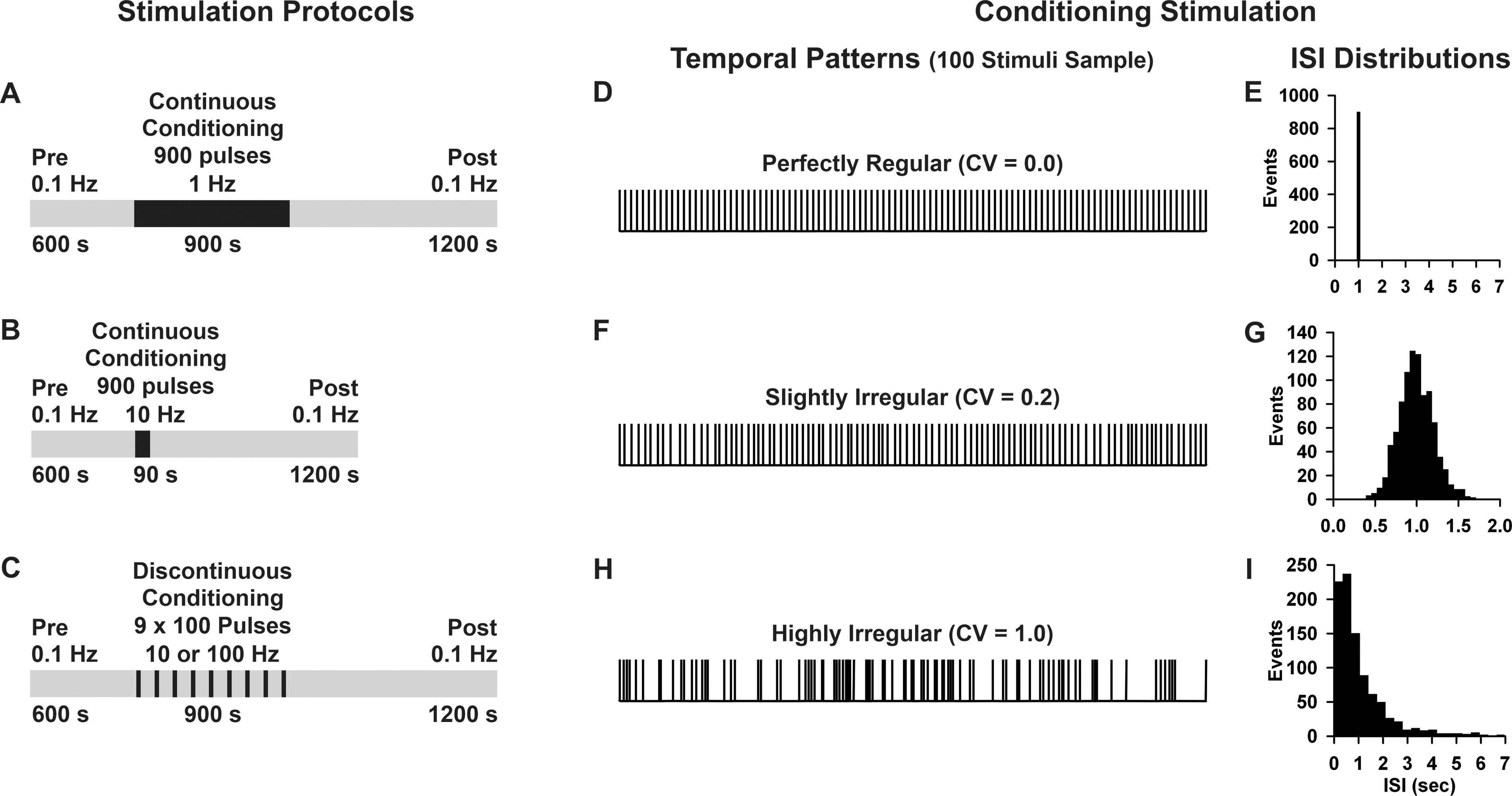
Stimulation protocols, temporal patterns, and interstimulus interval distributions. (A–C) Stimulation protocols for: 1 Hz continuous, 10 Hz continuous, and 10 Hz (or 100 Hz) discontinuous conditioning, respectively. Gray bands represent pre- and postconditioning periods, whereas black bands represent intervals of conditioning stimulation. Note that for the discontinuous stimulation protocols shown in (C) the conditioning period consists of alternating stimulation epochs (black bands) and rest intervals (gray bands). Rest intervals (10 Hz = 101.25 sec each, 100 Hz = 111.372 sec each) have probe trials at 0.1 Hz. (D–E) Example of perfectly regular conditioning (D), with all ISIs equal (E). (F–G) Example of slightly irregular conditioning (F), where ISIs have a Gaussian distribution (G). (H–I) Example of highly irregular conditioning (H), where ISIs have a Poisson distribution (I). Note that the times shown in panels (E), (G), and (I) are based on 1 Hz stimulation (10 Hz or 100 Hz stimulation are identical in pattern, but 10 or 100 times shorter in duration, respectively). ISI, interstimulus intervals.

Temporal patterns of conditioning stimulation

Conditioning stimulation temporal patterns were generated by creating ISIs according to the family of distributions given by: $P (t) \propto e^{- t^{2} / 2 η^{2}} e^{- t / τ_{d}} θ (t > τ_{R})$ (1)where τ_R is the refractory period, and η (>0) and τ_d are temporal parameters that govern the single peak of the distribution. For a perfectly regular distribution, we had -τ_d/η ≫ 1, and for a highly irregular distribution η/τ_d ≫ 1. We solved for the parameters η and τ_d, to yield a desired mean, m, and standard deviation (std) or CV: $\frac{{std}^{2}}{m^{2}} = \frac{Q {(w)}^{2} + 2 w Q (w) - 2}{2 {(1 - w Q (w))}^{2}},$ (2) $m = τ_{R} + (η \sqrt{2}) (\frac{1 - w Q (w)}{Q (w)}),$ (3)where $Q (w) \equiv \sqrt{π} erfcx(w),$ and $w \equiv \frac{η}{τ_{d} \sqrt{2}} + \frac{τ_{R}}{η \sqrt{2}} .$ Because equations (2) and (3) are monotonic, one can invert the equations to find η and τ_d in terms of m and std. Thus, it was possible to change a set of ISIs at one CV to a related set of ISIs at another CV. The cumulative distribution function corresponding to the event probability distribution function given by equation (1) above is: $cdf(t) = 1 - \frac{erfc(w +(t - τ_{R}) / (η \sqrt{2}))}{erfc(w)} .$ (4)

We randomly assigned numbers drawn uniformly on the unit interval to ISIs in the following way. For each random number, r, we inverted equation (4) to find a t that represented an ISI affiliated with a given mean and CV. By specifying a different mean and CV (and therefore different η and τ_d, or equivalently, different η and w) in equation (4), we derived related sets of ISIs, using a single set of random numbers.

Analyzing electrophysiology data

We measured evoked PSP (or FP) peak amplitudes during the last 5 min of pre- and postconditioning (using pCLAMP) and calculated a post/pre ratio. We evaluated the effects of mTBI, as well as stimulus frequency, temporal pattern, and continuity on the induction of synaptic plasticity [defined as: LTD, a significant (p < 0.05, t-test) decrease (≥10%) in post/pre ratios; LTP, a significant increase (≥10%) in post/pre ratios; or no change (NC), post/pre ratios that changed <10% and/or were not significantly different]. For these same time periods (the last 5 min of pre- and postconditioning), we used pCLAMP to calculate the average PSP: half width (at half height), rise time (10–90%), and decay time (90-10%); as well as the membrane potential and input resistance for each cell.

We also analyzed the kinetic profiles of conditioning responses for individual recordings in the groups that showed a significant difference between control and mTBI. For continuous stimulation protocols, we took all data points generated during the conditioning period and calculated exponential and linear best fits, from which we determined the slope. For discontinuous stimulation protocols, best fits were calculated for each of the nine conditioning subepochs and the slopes averaged. Furthermore, we calculated the mean of all conditioning response amplitudes (average), as well as the average of the initial 10% (initial) and final 10% (final). For all recordings within a given stimulation protocol, a linear regression analysis was performed to determine the degree to which each factor (exponential slope, linear slope, average amplitude, initial amplitude, and final amplitude) was correlated with plasticity outcome (post/pre ratio).

Calcium imaging

In a subset of the WC patch experiments, the ratiometric calcium sensitive dye Fura-4F (100 µM, Thermo Fisher Scientific) was added to the pipette solution. Baseline somatic calcium concentrations were calculated as the ratio of bound to unbound calcium minus background (AxioVision; Zeiss) during the last five minutes of preconditioning.

Statistics

We used SigmaPlot (Systat Software) to determine statistical significance, except where noted. Normality was assessed with a Shapiro–Wilk test. For normally distributed data, we used a t-test or an ANOVA followed by Fisher’s least significant difference method for multiple comparisons (Fischer’s LSD). For datasets with non-normal distributions, we used a Mann–Whitney U test (MWU) or a Kruskal–Wallis one-way ANOVA on ranks (Kruskal–Wallis) followed by Dunn’s method for multiple comparisons with Sidak correction (Dunn’s corrected; statskingdom.com/kruskal-wallis-calculator.html). Group data are presented as the mean ± SEM. To assess whether specific characteristics of conditioning responses were predictive of plasticity outcome, for each factor, we calculated a correlation coefficient and determined significance using linear regression. We considered differences statistically significant at p < 0.05 (except for Dunn’s correction, which was considered significant at p < 0.017).

Results

Efficacy of our mTBI model

To establish the efficacy of our CCI model for mTBI, we used several independent methods. First, we used a behavioral measure, recovery of righting reflex, to assess motor and cognitive function in control, sham, and mTBI rats. Righting latency was significantly impacted by treatment group (p = 0.04) and was longer in mTBI than in control (p = 0.04) or sham (p = 0.02; Fig. 2A) groups. Note that for this and all subsequent figures we show control data in black, sham data in blue, and mTBI data in red. Second, we measured intracellular calcium concentration in a subset of the L2/3 pyramidal neurons used for our WC patch-clamp recordings. Intracellular calcium concentrations were significantly different between treatment groups (p < 0.001) and were higher in the mTBI than in the control (p < 0.001) or sham group (p < 0.001; Fig. 2B). Third, we measured the intrinsic properties of this same subset of cells and found that input resistance was significantly affected by the treatment group (p = 0.005), being higher in the mTBI group than in the control (p = 0.001) or sham (p = 0.008; Fig. 2C) groups; whereas membrane potential did not differ between the control, sham, or mTBI groups (p = 0.38; Fig. 2D).

FIG. 2.

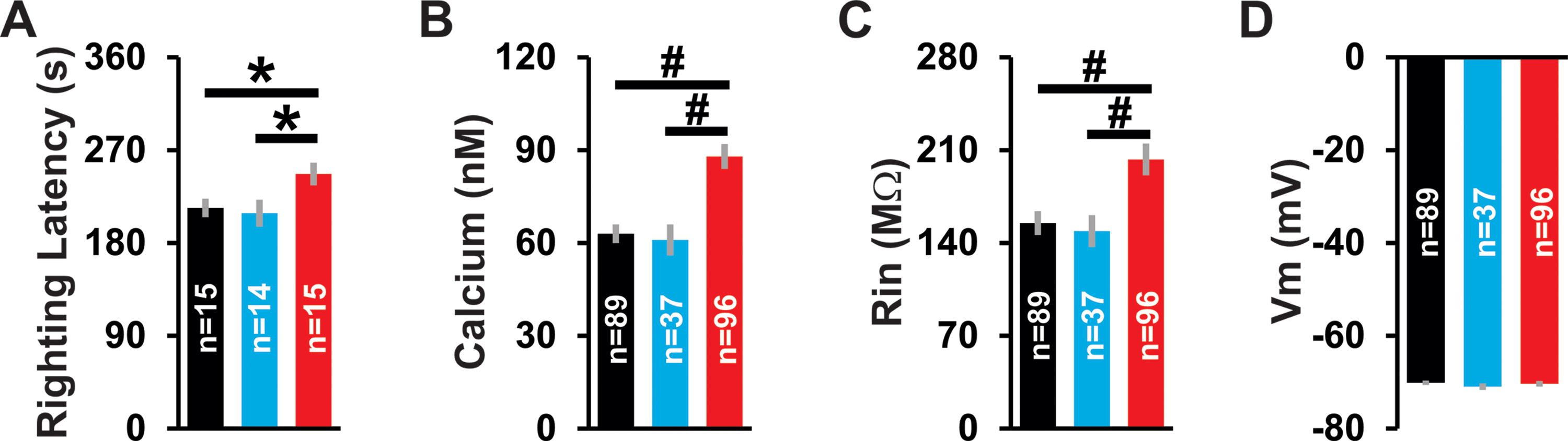
Efficacy of our CCI model for mTBI. (A) Righting latency, (B) intracellular calcium, and (C) input resistance are significantly increased in mTBI versus control or sham groups. The p values and statistical tests are: p = 0.04 ANOVA, p < 0.001 Kruskal–Wallis, p = 0.005 Kruskal–Wallis, respectively. Subsequent pairwise comparisons show significant differences: *p < 0.05 Fisher’s LSD, #p < 0.017 Dunn’s corrected. For this and all subsequent figures we show control data in black, sham data in blue, and mTBI data in red. Values are mean ± SEM, n = number of observations/group. (D) Membrane potential did not differ between treatment groups (control, sham, mTBI; p = 0.38 Kruskal–Wallis). CCI, controlled cortical impact; mTBI, mild traumatic brain injury.

Effect of temporal pattern and treatment condition on plasticity outcome

WC patch-clamp experiments were conducted to investigate the role of temporal pattern on synaptic plasticity in control, sham, and mTBI groups. Figure 3 shows example recordings of evoked PSPs and time plots of individual recordings in response to 1 Hz continuous highly irregular conditioning (cf. Fig. 1A, 1H-I). Note the substantial decrease in postconditioning PSP amplitude, indicative of LTD, in control and sham examples (Fig. 3A–B). In contrast, there was a substantial increase in postconditioning PSP amplitude, indicative of LTP, in the mTBI example (Fig. 3C).

FIG. 3.

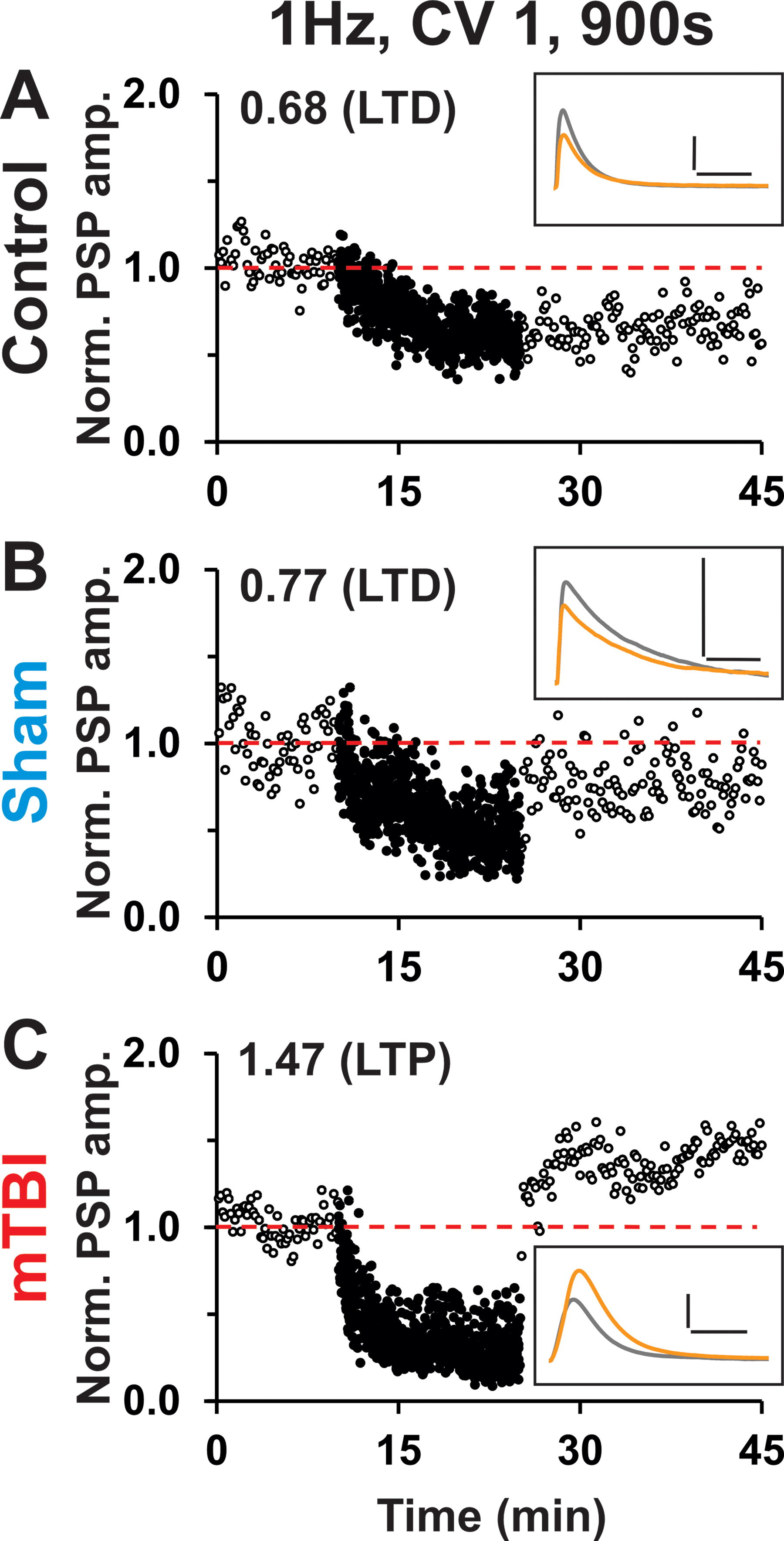
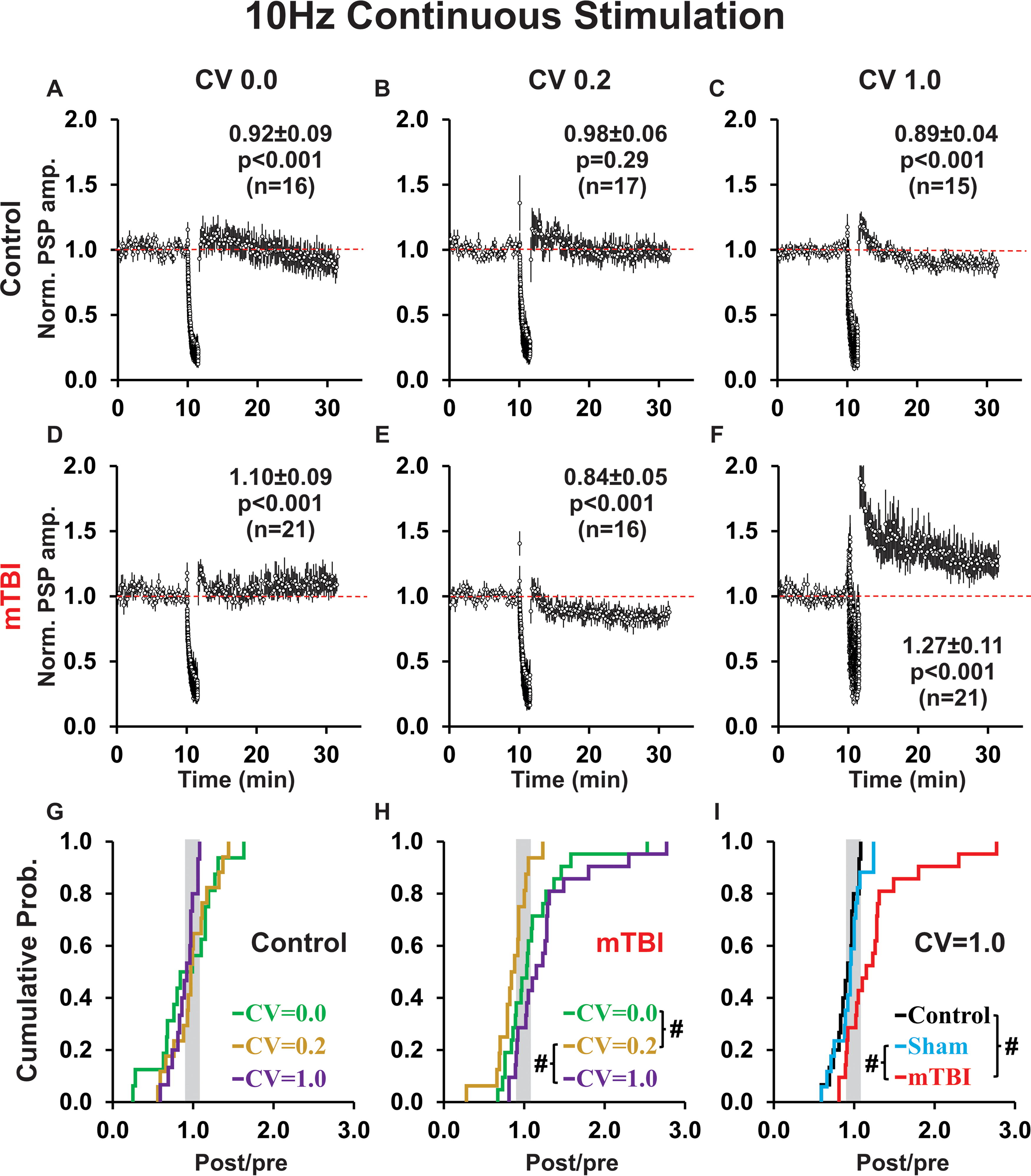
Individual time plots of WC responses to highly irregular 1 Hz continuous conditioning. (A–C) Representative examples from: control, sham, and mTBI groups. Black open circles = pre-/post-conditioning responses, black filled circles = conditioning responses, red dotted line = baseline. Numerical values = post/pre ratios and corresponding plasticity outcome (LTD, NC, or LTP). Insets: PSP waveforms averaged over the last 5 min of pre- (gray) or post- (orange) conditioning (scale bars: 5 mV, 50 ms). mTBI, mild traumatic brain injury; WC, whole-cell; LTP, long-term potentiation, LTD; long-term depression; NC, no change.

Grouped results for our WC recording experiments for the various frequencies, temporal patterns, and treatment groups are shown in subsequent figures. Continuous conditioning at 1 Hz induced LTD in both control groups (Fig. 4A–C) and mTBI groups (Fig. 4D–E) in all cases except one—highly irregular conditioning (CV 1.0) in mTBI rats resulted in LTP (Fig. 4F). Temporal pattern (CV 0.0, CV 0.2, CV 1.0) had no effect on plasticity outcome in control groups (p = 0.50; Fig. 4A–C, 4G). However, for mTBI groups, there was a significant difference in plasticity outcome between the three temporal patterns (p = 0.002; Fig. 4D–F, H) with highly irregular conditioning (CV 1.0) showing significant potentiation (versus: CV 0.0 p = 0.007, CV 0.2 p < 0.001). Notably, within each of the six stimulation groups, there was heterogeneity in plasticity outcomes among individual cells (Fig. 4G–H). Importantly, plasticity outcomes in control and mTBI rats were significantly different only when the temporal pattern was highly irregular (p = 0.008; cf. Fig. 4C, F), but not when it was perfectly regular (p = 0.76; cf. Fig. 4A, D) or slightly irregular (p = 0.66; cf. Fig. 4B, E). For highly irregular conditioning control, sham and mTBI groups were significantly different (p = 0.004; Fig. 4I). Pairwise comparisons showed that mTBI was significantly different from both control (p = 0.002) and sham (p = 0.002), but control and sham groups did not differ (p = 0.49; Fig. 4I). The potentiation produced by highly irregular 1 Hz conditioning in mTBI rats reflects both an increase in the proportion (control = 18%, sham = 6%, mTBI = 47%) and magnitude (post/pre ratio: control = 1.31, sham = 1.13, mTBI = 1.62) of LTP outcomes (Fig. 4I).

FIG. 4.

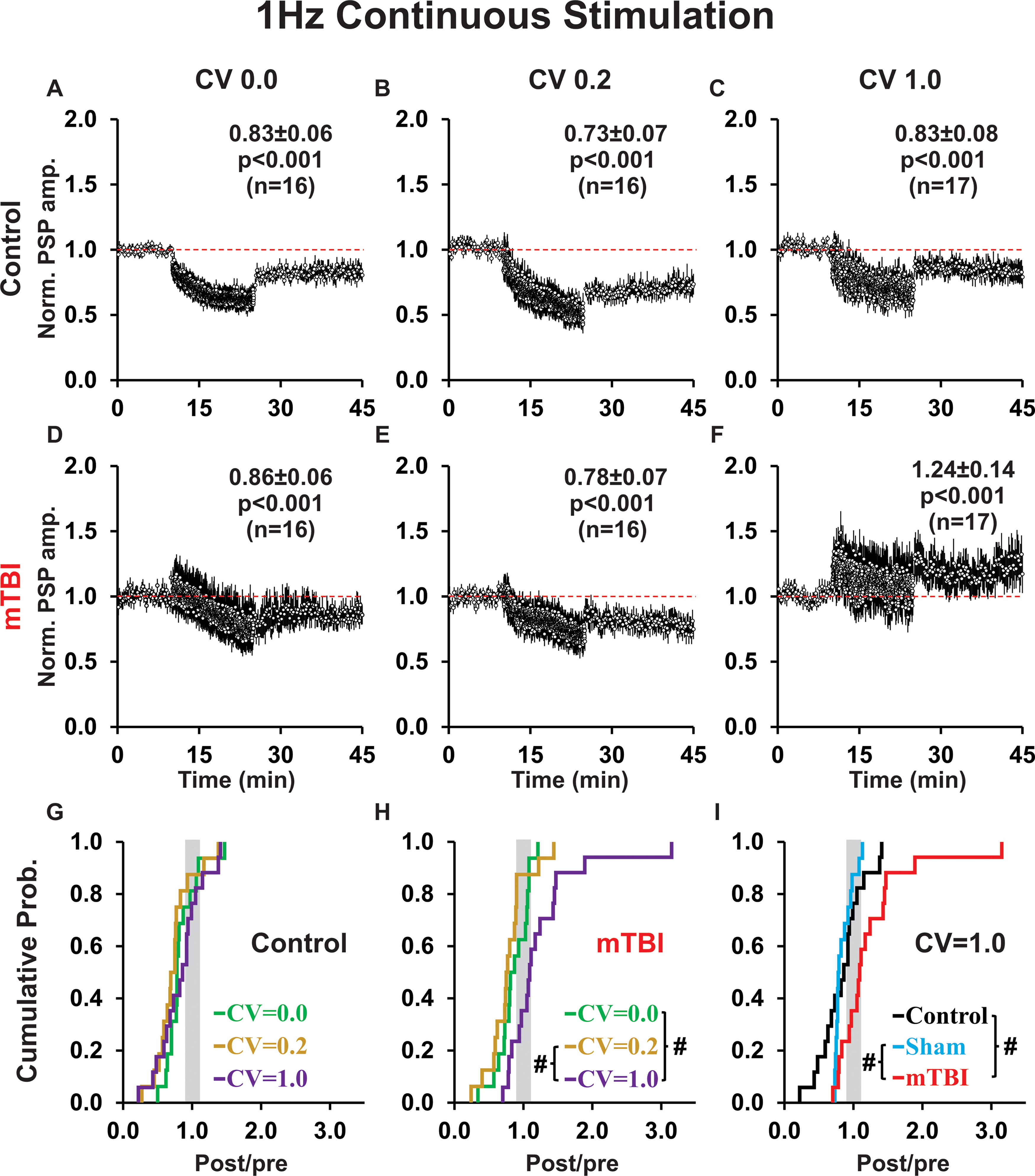
Continuous 1 Hz conditioning induces LTD in every case except one—highly irregular conditioning in mTBI rats results in LTP. (A–C) Mean time plots for control groups with: perfectly regular (CV 0.0), slightly irregular (CV 0.2), and highly irregular (CV 1.0) conditioning. Inset text: mean post/pre ratio ± SEM, p-values (t-test comparing the last 5 min of pre- vs. postconditioning), and n = number of cells. Red dashed line = baseline. (D–F) Mean time plots for mTBI groups. Note that control and mTBI groups differ for highly irregular (p = 0.008 MWU), but not perfectly regular (p = 0.76 t-test) or slightly irregular (p = 0.66 t-test) conditioning. (G–H) Cumulative probability plots of post/pre ratios in control groups and mTBI groups. Data steps falling: in the gray region show NC, to the left show LTD, and to the right show LTP. In control groups, temporal pattern had no appreciable effect (p = 0.50 ANOVA) on plasticity outcome (curves overlap). However, in mTBI groups, temporal pattern significantly impacted plasticity (p = 0.002 Kruskal–Wallis), with pairwise comparisons showing significant potentiation only for highly irregular conditioning: #p < 0.017 Dunn’s corrected. (I) Cumulative probability plots of post/pre ratio for highly irregular conditioning show a significant effect of treatment group (p = 0.004 Kruskal–Wallis, including 16 shams), with subsequent pairwise comparisons revealing a significant shift toward LTP after mTBI: #p < 0.017 Dunn’s corrected. mTBI, mild traumatic brain injury; LTP, long-term potentiation, LTD; long-term depression; MWU, Mann–Whitney U test.

In addition, highly irregular 1 Hz continuous conditioning differentially affected the evoked PSP shape indices (Supplementary Fig. S1A) in controls, showing a significant decrease in decay time (DT p = 0.03) and half width (HW p = 0.03; Supplementary Fig. S1B), and this effect occurred primarily in the responses that underwent LTD (DT p = 0.045, HW p = 0.03; Supplementary Fig. S1C, cf. Supplementary Fig. S1B, S1D). Shape indices in shams showed a similar decrease in DT (p = 0.09) and HW (p = 0.02; Supplementary Fig. S1B), which occurred primarily in responses that underwent LTD (DT p = 0.03, HW p = 0.02; Supplementary Fig. S1C, cf. Supplementary Fig. S1B, S1D). Interestingly, although the shape indices of the responses in the mTBI group as a whole did not change significantly after conditioning (DT p = 0.49, HW p = 0.54; Supplementary Fig. S1B), among just the responses that underwent LTP, they significantly increased (DT p = 0.01, HW p = 0.01; Supplementary Fig. S1D, cf. Supplementary Fig. S1B-C).

Continuous conditioning at 10 Hz produced a rapid rundown in PSP amplitudes, but was less likely to induce LTD, than 1 Hz continuous conditioning (cf. Figs. 5A–E, 4A–E). In particular, for controls, slightly irregular continuous conditioning produced LTD for 1 Hz, but NC for 10 Hz conditioning (p = 0.01; cf. Figs. 4B, 5B); whereas after mTBI, perfectly regular conditioning induced LTD for 1 Hz continuous, but LTP for 10 Hz continuous conditioning (p = 0.05; cf. Figs. 4D, 5D). Temporal pattern had no effect on plasticity outcome in control groups (p = 0.58; Fig. 5A–C, 5G). However, for mTBI groups, there was a significant difference in plasticity outcomes (p = 0.002; Fig. 5D–F, 5H) between slightly irregular conditioning, which showed a shift toward LTD, and perfectly regular conditioning or highly irregular conditioning, both of which showed a shift toward LTP (p = 0.015; p < 0.001; Fig. 5H). In addition, we found that 10 Hz continuous conditioning (similar to 1 Hz continuous conditioning) produced significantly different plasticity outcomes for control and mTBI groups only when the temporal pattern of conditioning was highly irregular (p = 0.003; cf. Fig. 5C, F), but not perfectly regular (p = 0.35; cf. Fig. 5A, D) or slightly irregular (p = 0.10; cf. Fig. 5B, E). Accordingly, for highly irregular conditioning, we analyzed control, sham, and mTBI groups (p = 0.003; Fig. 5I). Pairwise comparisons showed a significant potentiation of responses in mTBI relative to control (p = 0.001) and sham (p = 0.004) groups, but no difference between controls and shams (p = 0.30). The potentiated response to highly irregular conditioning (like that observed for the 1 Hz continuous group) reflected a change in both the proportion (control = 0%, sham = 12%, mTBI = 52%) and magnitude (post/pre ratio: control = no LTP responses, sham = 1.24, mTBI = 1.56) of LTP outcomes. However, unlike 1 Hz continuous conditioning, there were no effects of 10 Hz continuous conditioning on the shape indices of PSP responses (data not shown).

FIG. 5.

Continuous 10 Hz (compared to 1 Hz) conditioning produces a rapid rundown in PSP amplitudes, is less likely to result in LTD in controls, and more likely to result in LTP after mTBI. (A–C) Mean time plots for control groups. (D–F) Mean time plots for mTBI groups. Control and mTBI groups differ for highly irregular (p = 0.003 MWU), but not perfectly regular (p = 0.35 MWU) or slightly irregular (p = 0.10 t-test) conditioning. (G–H) Cumulative probability plots of post/pre ratios for: control groups (G) and mTBI groups (H). In control groups, temporal pattern has no effect (p = 0.58 Kruskal–Wallis) on plasticity outcome (curves overlap). However, in mTBI groups there is a significant effect of temporal pattern (p = 0.002 Kruskal–Wallis), with subsequent pairwise comparisons showing significant potentiation for both perfectly regular and highly irregular conditioning: #p < 0.017 Dunn’s corrected. (I) Cumulative probability plots of post/pre ratio for highly irregular conditioning show a significant effect of treatment group (p = 0.003 Kruskal–Wallis, including 17 shams), with subsequent pairwise comparisons revealing a significant shift toward LTP after mTBI: #p < 0.017 Dunn’s corrected. mTBI, mild traumatic brain injury; LTP, long-term potentiation, LTD; long-term depression; MWU, Mann–Whitney U test; PSP, postsynaptic potential.

For 10 Hz discontinuous stimulation protocols, the brief conditioning subepochs mitigated the rundown of response amplitudes that occurred for 10 Hz continuous conditioning protocols (cf. Figs. 6A–F, 5A–F). Moreover, probe stimuli administered at 0.1 Hz during the rest periods (Fig. 6A–F, yellow symbols) showed that PSP amplitudes quickly recovered, in most cases showing a brief period of post-tetanic potentiation, which suggests that any synaptic fatigue induced by an individual subepoch of higher frequency conditioning was transitory. Interestingly, probe trail response amplitudes were sensitive to the temporal pattern of conditioning in control groups (depressed for CV 0.0 and 1.0, but potentiated for CV 0.2; cf. Fig. 6A–C) and mTBI groups (potentiated for CV 0.0, neutral for CV 0.2, and potentiated for CV 1.0; cf. Fig. 6D–F). Notably, the continuity of 10 Hz conditioning influenced plasticity outcome and this was also dependent on temporal pattern. In controls, 10 Hz highly irregular conditioning induced a significantly more robust LTD when conditioning was discontinuous rather than continuous (p = 0.02; cf. Figs. 5C, 6C). In mTBI groups, 10 Hz perfectly regular conditioning induced LTD for discontinuous conditioning, but LTP for continuous conditioning (p = 0.06 trend; cf. Figs. 5D, 6D).

FIG. 6.

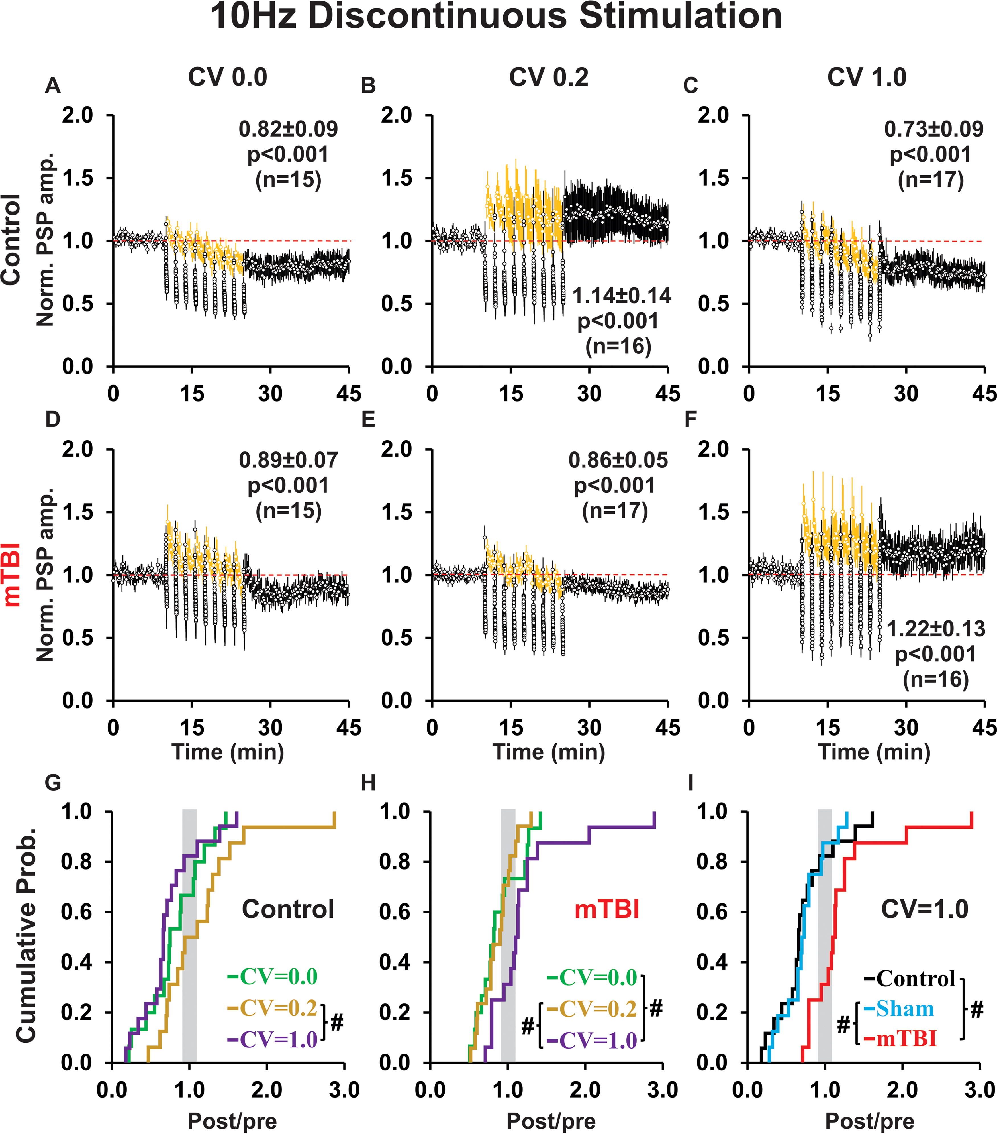
Discontinuous 10 Hz conditioning primarily induced LTD, except for slightly irregular conditioning in controls and highly irregular conditioning in mTBI rats. (A–C) Mean time plots for control groups. Note the eight rest periods of 101.25 s (consisting of probe trials at 0.1 Hz, yellow circles), evenly spaced between the nine conditioning subepochs (10 s at 10 Hz, black circles). (D–F) Mean time plots for mTBI groups. Note that control and mTBI groups differ for highly irregular (p < 0.001 MWU), but not perfectly regular (p = 0.56 t-test) or slightly irregular (p = 0.17 MWU) conditioning. (G–H) Cumulative probability plots of post/pre ratios for control groups (G) and mTBI groups (H). In control groups there is a significant effect of temporal pattern (p = 0.04 Kruskal–Wallis), with pairwise comparisons showing a significant difference between slightly irregular conditioning (showing LTP) and highly irregular conditioning (showing LTD): #p < 0.017 Dunn’s corrected. In mTBI groups, there is a significant effect of temporal pattern (p = 0.02 Kruskal–Wallis), with pairwise comparisons showing a significant shift toward LTP for highly irregular conditioning: #p < 0.017 Dunn’s corrected. (I) Cumulative probability plots of post/pre ratio for highly irregular conditioning show a significant effect of treatment group (p < 0.001 Kruskal–Wallis, including 16 shams), with subsequent pairwise comparisons revealing a significant shift toward LTP after mTBI: #p < 0.017 Dunn’s corrected. mTBI, mild traumatic brain injury; LTP, long-term potentiation, LTD; long-term depression; MWU, Mann–Whitney U test.

For 10 Hz discontinuous (unlike 10 Hz continuous) conditioning, there was a significant effect of temporal pattern between control groups (p = 0.04; Fig. 6A–C, 6G), as well as between mTBI groups (p = 0.02; Fig. 6D–F, H). Pairwise comparisons showed a significant effect of temporal pattern in controls, with LTD in response to highly irregular conditioning (Fig. 6C) compared to LTP elicited by slightly irregular conditioning (p = 0.006; Fig. 6B, G). In mTBI groups, there was a significant difference between highly irregular (Fig. 6F) and both: slightly irregular (p = 0.006; Fig. 6E, H) and perfectly regular (p = 0.012; Fig. 6D, H) conditioning. Moreover, control and mTBI groups differed for highly irregular conditioning (p < 0.001; cf. Fig. 6C, F), but not for slightly irregular (p = 0.17; cf. Fig. 6B, E) or perfectly regular (p = 0.56; cf. Fig. 6A, D) conditioning. Accordingly, for highly irregular conditioning, we analyzed control, sham, and mTBI groups (p < 0.001; Fig. 6I). Pairwise comparisons showed a significant difference between treatment groups—with a robust shift toward LTP in mTBI relative to both control (p < 0.001) and sham (p < 0.001) groups (Fig. 6I). The potentiation reflected an increase in the proportion (control = 12%, sham = 12%, mTBI = 56%), but (unlike 1 Hz and 10 Hz continuous conditioning) not magnitude (post/pre ratio: control = 1.50, sham = 1.23, mTBI = 1.48) of LTP outcomes. There were no effects of 10 Hz discontinuous conditioning on PSP shape indices (data not shown).

For 100 Hz conditioning, we used only a discontinuous protocol which allowed for rapid recovery of PSP amplitudes during rest intervals [with attendant enduring post-tetanic potentiation-see yellow probe trial data during conditioning (gray bar)-Figure 7A–F]. Note that data from the nine conditioning subepochs are not shown because most PSPs were embedded in a wave of depolarization and/or had ISIs too short to allow accurate quantification. In control groups, 100 Hz discontinuous perfectly regular and slightly irregular conditioning produced no change in PSP amplitude (cf. Fig. 7A, B), whereas highly irregular conditioning induced LTD (Fig. 7C) similar to 1 Hz continuous, 10 Hz continuous, and 10 Hz discontinuous conditioning (cf. Figs. 7C, 4C, 5C, 6C). In contrast, for mTBI groups, perfectly regular conditioning produced NC (Fig. 7D), slightly irregular conditioning produced LTP ([Fig. 7E], which differed from 1 Hz continuous, 10 Hz continuous, and 10 Hz discontinuous conditioning, all of which exhibited LTD [cf. Figs. 7E, 4E, 5E, 6E]), and highly irregular 100 Hz continuous conditioning resulted in NC (Figure 7F; which differed from 1 Hz continuous, 10 Hz continuous, and 10 Hz discontinuous conditioning—all of which induced LTP [cf. Figs. 4F, 5F, 6F]). Importantly, despite these modest differences, comparisons between control groups (p = 0.17) or between mTBI groups (p = 0.93) showed no significant effect of temporal pattern on plasticity outcome for the 100 Hz discontinuous conditioning protocol. In addition, there was no significant difference in plasticity outcomes between control and mTBI groups for any temporal pattern (CV 0.0 p = 0.40, CV 0.2 p = 0.97, CV 1.0 p = 0.28).

FIG. 7.

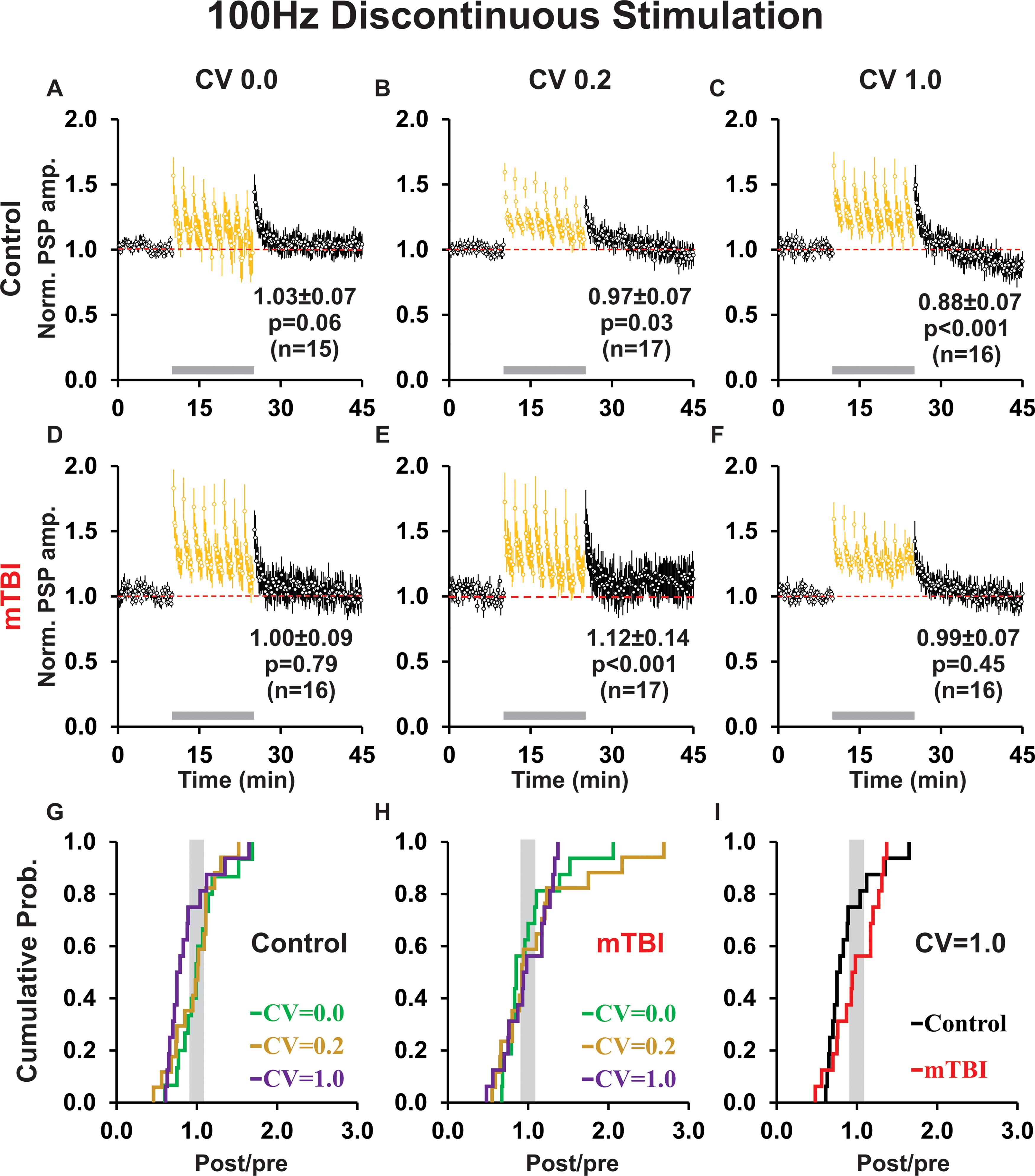
Discontinuous 100 Hz conditioning resulted in little plasticity, except for highly irregular conditioning in controls which produced LTD and slightly irregular conditioning after mTBI which induced LTP. (A–C) Mean time plots for control groups. Gray bars indicate the conditioning period which consisted of nine conditioning subepochs (1 s at 100 Hz) interspersed between eight evenly spaced rest periods of 131.25 s (with probe trials at 0.1 Hz, yellow symbols). Note that data for conditioning subepochs are not shown because the brevity of ISIs precluded measurement of most PSP peak amplitudes. (D–F) Mean time plots for mTBI groups. There was no difference in plasticity outcome between control and mTBI groups for any temporal pattern (CV 0.0: p = 0.40 MWU, CV 0.2: p =0.97 MWU, CV 1.0: p = 0.28 t-test). (G–H) Cumulative probability plots of post/pre ratios for: control groups (G) and mTBI groups (H). There was no effect of temporal pattern on plasticity outcome: between control groups (p = 0.17 Kruskal–Wallis) or between mTBI groups (p = 0.93 Kruskal–Wallis). (I) Cumulative probability plots of post/pre ratio for highly irregular conditioning in control and mTBI groups. Note that for 100 Hz discontinuous (unlike 1 Hz continuous, 10 Hz continuous, and 10 Hz discontinuous) highly irregular conditioning, plasticity outcome was not significantly affected by treatment group (control vs. mTBI, p = 0.28 t-test). mTBI, mild traumatic brain injury; LTP, long-term potentiation, LTD; long-term depression; MWU, Mann–Whitney U test; PSP, postsynaptic potential; CV, coefficient of variation; ISI, interstimulus interval.

Interestingly, for 100 Hz highly irregular conditioning, the shape indices of PSPs among the mTBI group showed a significant increase in HW overall (p = 0.03; Supplementary Fig. S1E) that was nonspecific for plasticity outcome (LTD p = 0.40, LTP p = 0.26; cf. Supplementary Fig. S1E-G), whereas in controls there was no significant change in DT overall (p = 0.54; Supplementary Fig. S1E), but a significant decrease for those cells responding with LTP (p = 0.04; Supplementary Fig. S1G) but not LTD (p = 0.39; Supplementary Fig. S1F). In contrast, for 100 Hz slightly irregular (CV = 0.2) conditioning, the mTBI group showed an increase in RT overall (p = 0.002; Supplementary Fig. S1H) which was consistent across all plasticity outcomes (LTD p = 0.035, LTP p = 0.006; cf. Supplementary Fig. S1H-J), whereas in controls RT was unchanged overall (p = 0.06) or for any particular plasticity outcome (LTD p = 0.18, LTP p = 0.47; cf. Supplementary Fig. S1H-J).

Kinetic properties of conditioning period responses

We analyzed the kinetic profiles of conditioning responses for individual recordings, in the groups that showed a significant difference between control and mTBI, to determine if they were predictive of plasticity outcome. For 1 Hz continuous highly irregular conditioning, we show example time plots of conditioning responses for each treatment group (Fig. 8A–C). Notably, the slope of an exponential best fit of conditioning response amplitudes showed a significant correlation with plasticity outcomes only in control (p = 0.02; Fig. 8A, D) and sham groups (p = 0.048; Fig. 8B, D), whereas the slope of a linear best fit showed a significant correlation with plasticity outcomes only in the mTBI group (p = 0.02; Fig. 8C, E). The slopes of conditioning response amplitudes did not significantly differ in magnitude for either linear (control = −0.013 ± 0.003, sham = −0.012 ± 0.003, mTBI = −0.007 ± 0.004; p = 0.41 ANOVA; data not shown) or exponential best fits (control = −0.019 ± 0.005, sham = −0.018 ± 0.004, mTBI = −0.011 ± 0.004; p = 0.39 ANOVA; data not shown). However, relative to control and sham groups, the mTBI group exhibited a significant increase in conditioning response amplitude: initial value (overall p = 0.002, mTBI vs. control p < 0.001, mTBI vs. sham p = 0.003), final value (overall p = 0.006, mTBI vs. control p = 0.001, mTBI vs. sham p = 0.007), and average value (overall p = 0.01, mTBI vs. control p = 0.003, mTBI vs. sham p = 0.019—trend; Fig. 8F). In addition, in the mTBI group, all of these values: average (p = 0.004), initial value (p = 0.007), and final value (p = 0.001) were predictive of plasticity outcome (Fig. 8G-I), whereas in the control and sham groups, only the average (control p = 0.04, sham p = 0.03) and final (control p = 0.007, sham p = 0.009) amplitudes were predictive of plasticity outcome (Fig. 8G-I).

FIG. 8.

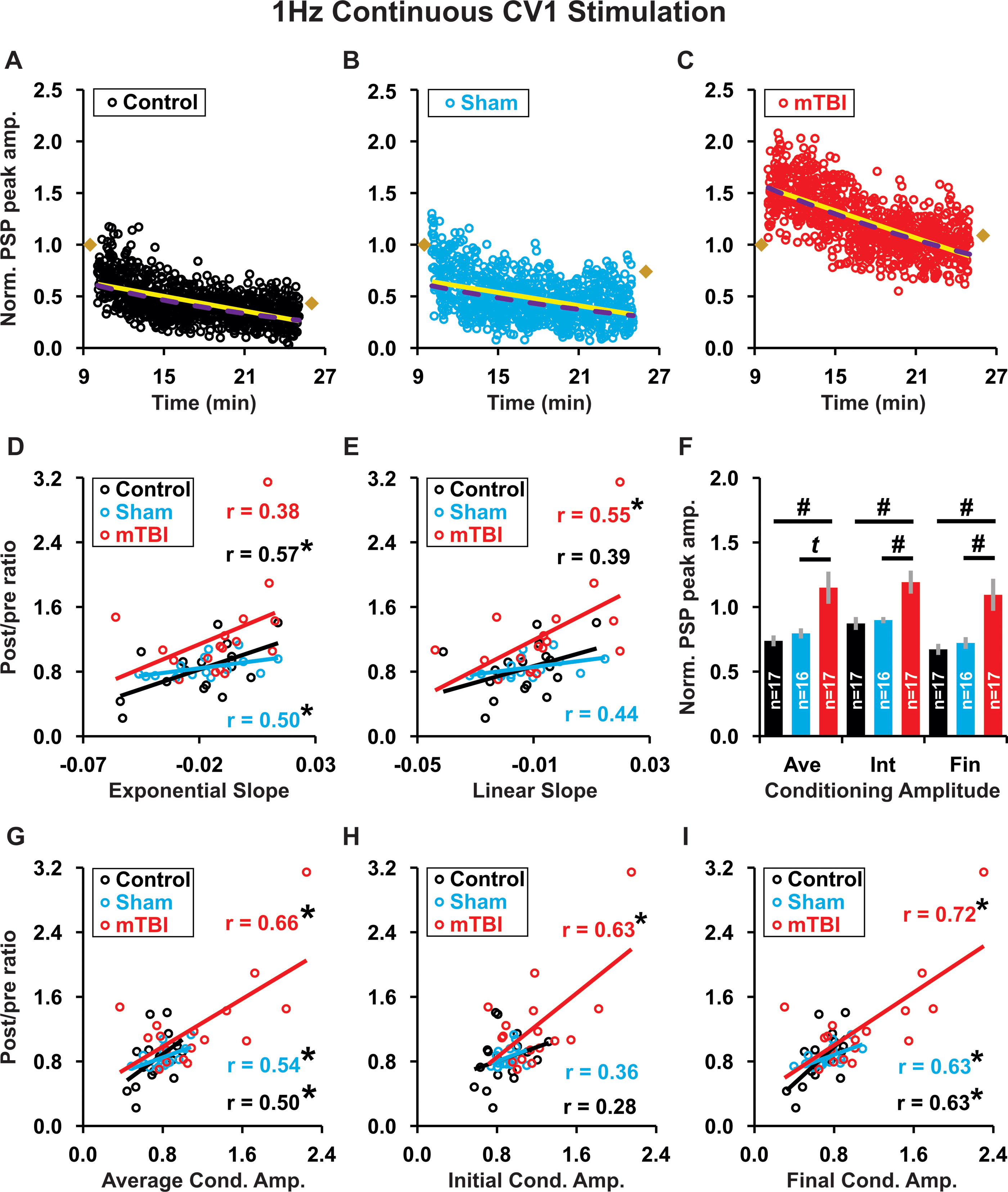
During 1 Hz continuous highly irregular conditioning, the kinetic profile of response amplitudes was predictive of plasticity outcome. (A–C) Individual time plots of conditioning period normalized PSP peak amplitudes for representative examples from: control, sham, and mTBI groups. Tan diamonds in each plot show the average of normalized PSP peak amplitudes for the last 5 min of the preconditioning (left) and the last 5 min of the postconditioning (right). For each time plot we calculated the exponential best fit (purple dashed line) and linear best fit (yellow solid line) to obtain the exponential and linear slopes, respectively. (D–E) Plots of post/pre ratio (plasticity outcome) versus: exponential slope (D) and linear slope (E) (control n = 17, sham n = 16, mTBI n = 17; for this and subsequent panels). r = correlation coefficient. Note that the conditioning slope shows a significant correlation for: an exponential fit only in the control and sham groups and a linear fit only in the mTBI group. *p < 0.05 linear regression. (F) Normalized PSP peak amplitude during conditioning: Ave (average of all data points), Int (initial 10% of data points averaged), and Fin (final 10% of data points averaged). Values are mean ± SEM. Inset text: n = the number of cells/group. Note that PSP amplitudes are increased in mTBI relative to control and sham groups. #p < 0.017 Dunn’s corrected. t = trend (p = 0.019 Dunn’s corrected). (G–I) Plots of post/pre ratio versus normalized PSP peak amplitude for: average, initial, and final values. Note that while all conditioning amplitudes (average, initial, and final) were significantly correlated with plasticity outcome in the mTBI group, only the average and final values were significantly correlated with plasticity outcome in the control and sham groups. *p < 0.05 linear regression. mTBI, mild traumatic brain injury; PSP, postsynaptic potential.

In contrast, for 10 Hz continuous highly irregular conditioning, the kinetics of the conditioning responses (slope Fig. 9A–E; amplitude: Fig. 9G-I) were not predictive of plasticity for any treatment group (control, sham, or mTBI). However, exponential best fits of conditioning amplitude had a shallower slope in mTBI than in control or sham groups (overall p < 0.001 ANOVA; with mTBI = −0.580 ± 0.096 vs. control = −1.045 ± 0.090, or sham = −1.125 ± 0.114; p = 0.002, p < 0.001, Fisher’s LSD; data not shown). Moreover, although the conditioning response amplitude was not significantly different between treatment groups initially (p = 0.15; Fig. 9F), both the average (overall p = 0.006, mTBI vs. control p = 0.009, mTBI vs. sham p = 0.002) and final (overall p < 0.001, mTBI vs. control p = 0.001, mTBI vs. sham p < 0.001) amplitudes were significantly higher in the mTBI group than in the control or sham groups (Fig. 9F). Thus, during 10 Hz continuous highly irregular conditioning, response amplitudes decreased less and more slowly in mTBI than in control and sham groups.

FIG. 9.

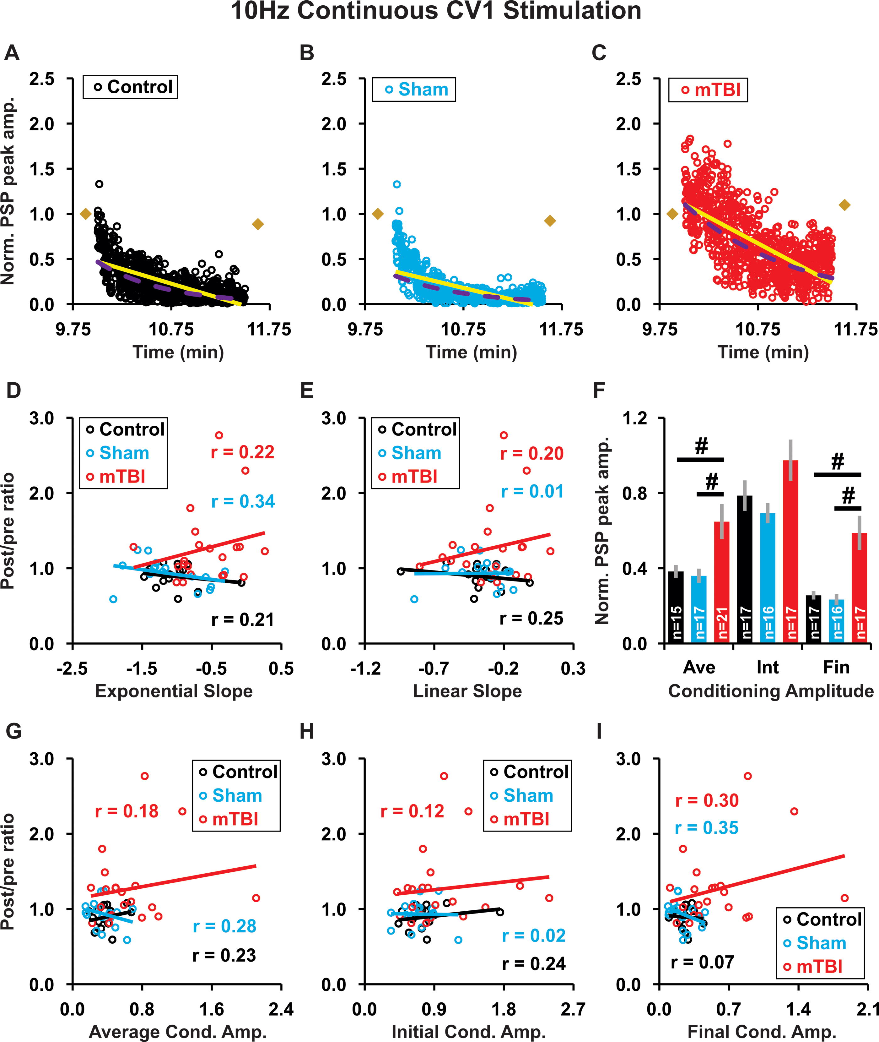
During 10 Hz continuous highly irregular conditioning, the kinetic profile of response amplitudes was not predictive of plasticity outcome. (A–C) Individual time plots of conditioning period normalized PSP peak amplitudes for representative examples from: control, sham, and mTBI groups. (D–E) Plots of post/pre ratio versus exponential slope (D), and linear slope (E) (control n = 15, sham n = 17, mTBI n = 21; for this and subsequent panels). r = correlation coefficient. Note that post/pre ratio shows no significant correlation with either exponential or linear slope (controls: p = 0.44, p = 0.38; shams: p = 0.18, p = 0.96; mTBI: p = 0.34, p = 0.37; linear regression). (F) Normalized PSP peak amplitude: average (Ave), initial (Int), and final (Fin) values. Note that although the initial amplitude was similar for all treatment groups (p = 0.15 Kruskal–Wallis), the average and final amplitudes were significantly increased after mTBI (p = 0.006, p < 0.001; Kruskal–Wallis). Subsequent pairwise comparisons: #p < 0.017, Dunn’s corrected. (G–I) Plots of post/pre ratio versus normalized PSP peak amplitude: average, initial, and final values. Post/pre ratio was not correlated with average, initial, or final amplitude for any treatment group (control: p = 0.41, 0.38, 0.82; sham: p = 0.28, 0.94, 0.18; mTBI: p = 0.43, 0.61, 0.19; linear regression). mTBI, mild traumatic brain injury; PSP, postsynaptic potential.

For 10 Hz discontinuous highly irregular conditioning, the kinetic profile of conditioning response amplitudes measured as the average slope of exponential or linear best fits (Fig. 10A–C) was predictive of plasticity outcome only in control and sham groups—showing significant negative correlations for both linear slope (control p < 0.001, sham p = 0.02) and exponential slope (control p < 0.001, sham p = 0.04; Fig. 10D–E). This result differs from both 1 Hz continuous highly irregular conditioning (significant positive correlation, cf. Fig. 8D–E) and 10 Hz continuous highly irregular conditioning (no correlation, cf. Fig. 9D–E). There was no significant difference in the magnitude of conditioning response slopes between treatment groups, for either: linear (control −0.560 ± 0.376, sham −0.908 ± 0.233, mTBI −1.157 ± 0.155; p = 0.19 Kruskal–Wallis; data not shown) or exponential best fits (control −0.899 ± 0.671, sham −1.555 ± 0.297, mTBI −1.959 ± 0.388; p = 0.24 Kruskal–Wallis; data not shown). In addition, there was no significant difference in the magnitude of conditioning response amplitude: average (p = 0.75), initial (p = 0.95), or final values (p = 0.41; Fig. 10F). However, in the mTBI group, conditioning response amplitude: average (p = 0.02), initial value (p = 0.03), and final value (p = 0.02) were all predictive of plasticity outcome (Fig. 10G-I). In contrast, for the control and sham groups, conditioning response amplitude was not predictive of plasticity outcome for: average (control p = 0.71, sham p = 0.35; Fig. 10G), initial (control p = 0.17, sham p = 0.24; Fig. 10H), or final values (control p = 0.69, sham p = 0.44; Fig. 10I).

FIG. 10.

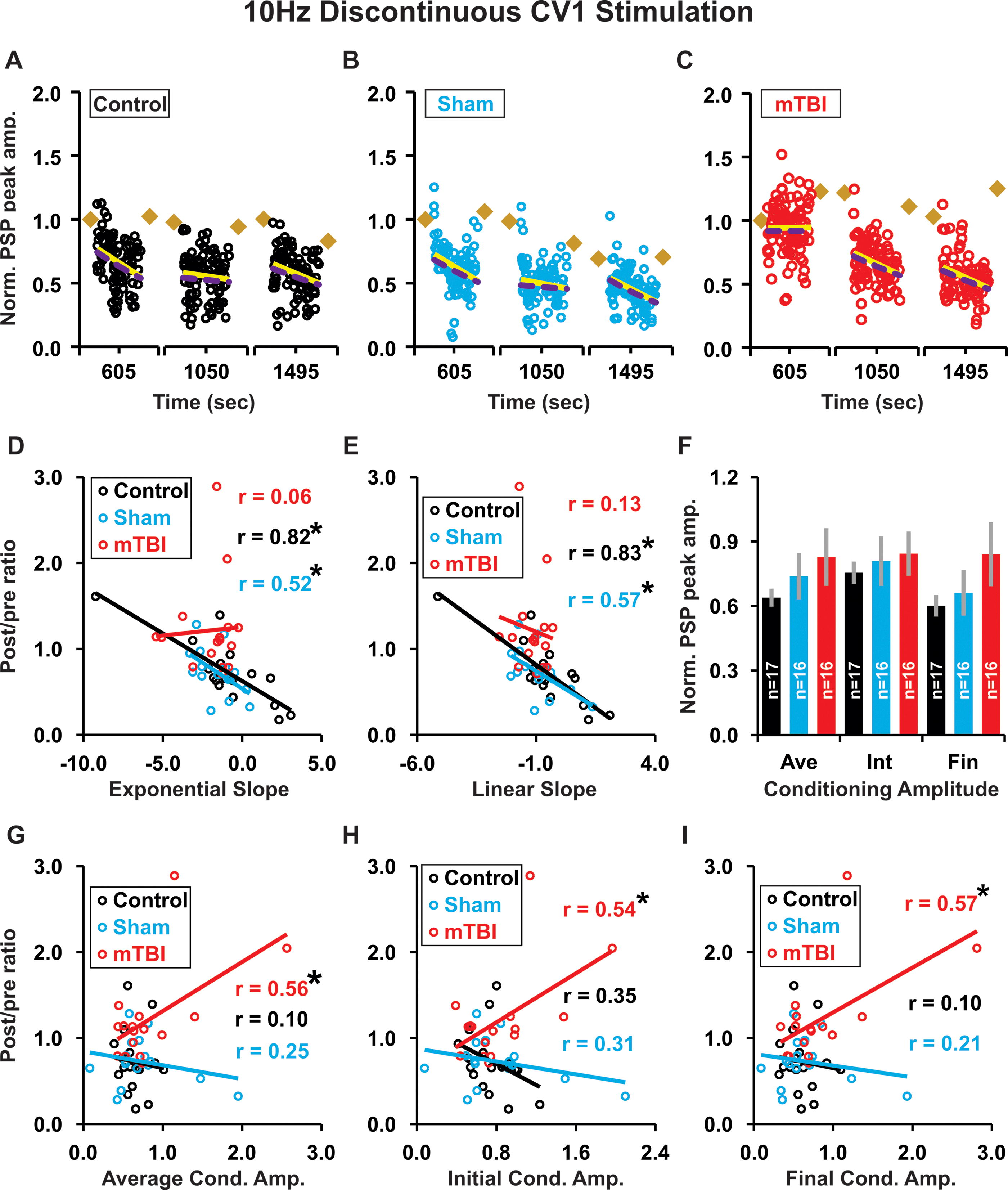
During 10 Hz discontinuous highly irregular conditioning, the kinetic profile of PSP responses had: slopes (exponential and linear) that were significantly correlated with plasticity outcome in control and sham, but not in mTBI groups; and amplitudes (average, initial and final) that were significantly correlated with plasticity outcome in mTBI groups, but not control or sham groups. (A–C) Individual time plots of conditioning period normalized PSP peak amplitudes for representative examples of: control, sham, and mTBI groups. Note that only the first (left), fifth (center), and ninth (right) conditioning subepochs are shown. Tan diamonds represent the average of normalized PSP peak amplitudes for (from left to right): the last 5 min of preconditioning and the first rest interval (left), the fourth and fifth rest intervals (center), and the eighth rest interval and the last 5 min of postconditioning (right). For each conditioning subepoch we calculated the exponential best fit (purple dashed line) and linear best fit (yellow solid line) to obtain the exponential and linear slopes. (D–E) Plots of post/pre ratio versus conditioning slope (average of all 9 conditioning subepochs) for exponential (D) and linear (E) best fits, respectively (control n = 17, sham n = 16, mTBI n = 16; for this and subsequent panels). r = correlation coefficient. Note that the conditioning slopes (exponential and linear) show a significant negative correlation with plasticity outcome in control (p < 0.001, p < 0.001) and sham (p = 0.04, p = 0.02), but not mTBI (p = 0.84, p = 0.64) groups. *p < 0.05, linear regression. (F) Normalized PSP peak amplitude: average (Ave), initial (Int), and final (Fin) values. Treatment group (control, sham, mTBI) had no effect on average (p = 0.75 Kruskal–Wallis), initial (p = 0.95 Kruskal–Wallis), or final amplitude (p = 0.41 Kruskal–Wallis). (G–I) Plots of post/pre ratio versus normalized PSP peak amplitude: average, initial, and final values. Conditioning amplitudes (average, initial, and final) showed a significant positive correlation with plasticity outcome in the mTBI (p = 0.03, 0.04, 0.03), but not the control (p = 0.71, 0.17, 0.69) or sham group (p = 0.35, 0.24, 0.44; linear regression). *p < 0.05 linear regression. mTBI, mild traumatic brain injury; PSP, postsynaptic potential.

Data from our WC recordings appear broadly representative

In order to assess whether our WC results were reflective of the larger population of synapses in L2/3, we also made simultaneous FP recordings. Representative examples of individual recordings and time plots for paired WC and FP recordings are shown in Supplementary Figure S2 for: 1 Hz continuous (Supplementary Fig. S2A–B), 10 Hz continuous (Supplementary Fig. S2C-D), and 10 Hz discontinuous (Supplementary Fig. S2E-F) conditioning. Notably, plasticity was highly correlated between the simultaneous WC and FP recordings regardless of treatment group (control p < 0.001, sham p < 0.001, mTBI p < 0.001; Supplementary Fig. S2G) or temporal pattern (CV 0.0 p < 0.001, CV 0.2 p < 0.001, CV 1.0 p < 0.001; Supplementary Fig. S2H).

Discussion

We found that mTBI dramatically affected the dependency of plasticity on the temporal pattern of conditioning. At all frequencies studied, with highly irregular temporal patterns of synaptic conditioning, where neurons from controls underwent LTD (Fig. 4C, 5C, 6C, 7C), those from mTBI animals underwent LTP (for 1 Hz or 10 Hz; Fig. 4F, 5F, 6F) or NC (for 100 Hz; Fig. 7F). Moreover, with slightly irregular or perfectly regular temporal patterns of conditioning, neurons from mTBI animals underwent different plasticity outcomes than those from controls (LTP vs. NC for 10 Hz continuous conditioning, CV 0, cf. Fig. 5D, A; LTD vs. NC for 10 Hz continuous conditioning, CV 0.2, cf. Fig. 5E, B; and LTD vs. LTP for 10 Hz discontinuous conditioning, CV 0.2, cf. Fig. 6E, B). Finally, for slightly or highly irregular 100 Hz discontinuous conditioning, neurons from mTBI rats displayed different plasticity outcomes from controls (LTP vs. NC for CV 0.2, cf. Fig. 7E, B; and NC vs. LTD for CV 1.0, cf. Fig. 7D, A).

To our knowledge previous studies have not examined the effect of temporal pattern on the induction of LTP or LTD following TBI, but they have shown that temporal pattern affects induction of synaptic plasticity in the normal brain. Studies using 2 Hz Markovian stimulation with different second order statistics reported that strong negative correlations produced LTD, whereas more positive correlations produced LTP.^115
–117 In addition, studies using a spike timing dependent plasticity protocol evoked by paired pre-post synaptic stimulation at 0.5–3 Hz observed LTD if ISIs were regular or had a Gaussian distribution, but no plasticity (NC) if ISIs had a Poisson distribution.^118,119 A direct comparison with these studies is difficult because we used a different approach in generating our stimulation protocols, but one study¹²⁰ used a similar approach—varying the CV for ISIs—and similar to them, we found that 1 Hz perfectly regular conditioning produced LTD, but inconsistent with them, we found that 1 Hz highly irregular conditioning often did too. This discrepancy in plasticity outcomes for highly irregular conditioning may reflect subtle but important differences in the temporal pattern of ISIs in the two studies or could reflect differences in: stimulus pulse duration, species, or degree of brain maturation, including the development of synaptic inhibition.

Analyses of PSP shape index and conditioning response kinetics suggest underlying plasticity mechanisms in mTBI

Our WC patch clamp recordings of compound PSPs from L2/3 pyramidal neurons evoked by stimulation of L4 probably included a mixture of excitatory and inhibitory components to L2/3 pyramidal neurons.^121

–125 Therefore, changes in evoked PSP amplitude after conditioning could reflect an alteration in any of these components. For example, LTP of the PSP could be due to an increase in the strength of excitatory transmission, a decreased strength of inhibitory transmission, or both.

We chose not to pharmacologically isolate either component as we aimed to have the experiments directly address the type of neurostimulation that would be used in a clinical situation. However, we did apply an analysis of PSP shape indices^{120,126

–129} (half width, rise time, and decay time) to our WC recordings (Supplementary Fig. S1). These results were generally consistent with LTP of the PSP being due to an increase in excitatory transmission strength and LTD being due to a decrease in excitatory transmission strength. Moreover, the FP results (Supplementary Fig. S2G–H) that are generally thought to reflect excitatory synaptic transmission^130,131 were consistent with this result.

Our results show that the frequency, continuity, and temporal pattern of conditioning stimulation interact to modify synaptic plasticity, but that interaction of these factors produces different plasticity outcomes in control (naive and sham) rats versus those with mTBI. Application of these results can also be informed by our findings on the utility of the kinetic profile of synaptic responses during the conditioning (Fig. 8–10) for predicting a desired plasticity outcome. Our utilization of probe trials (Fig. 6–7) to assess synaptic strength throughout the conditioning period could be useful to adapt a treatment protocol in real time to achieve the desired plasticity outcome.^{132

–137}

The increased intracellular calcium concentration and input resistance we observed following mTBI (Fig. 2) are indicative of increased neuronal excitability.^138,139 Evidence suggests that differences in the magnitude, duration, rate of rise, source, and spatial distribution of intracellular calcium signals are important for triggering LTD vs. LTP.^{134,140

–146} These distinct calcium signals may act differentially on downstream signaling cascades,^147

–151 to selectively alter postsynaptic AMPA receptors^{152

–157} and translation/transcription factors.^{158

–163} Moreover, intracellular calcium levels can increase over larger spatial and temporal scales, for example, by entry through voltage-gated calcium channels and/or release from intracellular stores,^164

–168 which can affect processes such as gene expression and protein synthesis that contribute to more persistent synaptic plasticity.^169

–172

Implications of our results for potential therapeutic interventions in the treatment of mTBI

One potential application of our findings is to inform the design of stimulation parameters for clinical interventions such that different patterns of synaptic conditioning characterized by specific combinations of temporal pattern, frequency, and continuity could be deployed to modulate plasticity outcomes, strengthening or weakening affected neural circuits, to promote recovery of cortical function after mTBI. Recent clinical studies have demonstrated the efficacy of neurostimulation for treatment of several neurological and psychiatric conditions, including the use of: tES for Parkinson’s disease,¹⁷³ Alzheimer’s disease,¹⁷⁴ seizures,¹⁷⁵ OCD,⁸³ and major depression;^176
–178 TMS for Alzheimer’s disease,¹⁷⁴ OCD,⁸¹ and postconcussive symptoms;¹⁷⁹ and DBS for Parkinson’s disease,¹⁸⁰ seizure disorders,¹⁸¹ OCD,¹⁸² and major depression.^183
–185 However, the relationship of various stimulation parameters to treatment efficacy is not well understood.¹⁸⁶ In order to optimize such approaches, the identification of the most effective stimulation parameters, including those that may elicit desired up- or downregulation of downstream synaptic networks, would be useful. Indeed, emerging methods and technologies for different stimulation modalities—DBS,^{89,187
–189} TMS,¹⁹⁰ tES,¹⁹¹ tFUS^192
–194—have the potential to provide new insights for optimizing neurostimulation protocols. In addition, TMS, tES, and tFUS have the important advantage of eliminating the need for invasive brain surgery.

Limitations and future directions

Our study design encompassed an extensive parameter space, comprised not only of different treatment groups (control, sham, mTBI) but also different stimulation as follows: frequencies (1, 10, and 100 Hz), temporal patterns (perfectly regular, slightly irregular, highly irregular), and continuities (continuous, discontinuous). Because of this, we chose to constrain several other factors, including: sex (we used only males), age at injury (8–9 weeks), and the duration of recovery (2–3 weeks). As our study was confined to males, it remains to be determined whether similar effects would occur in females as reports have indicated time- and sex-dependent differences in cerebrovascular responses to mTBI in rodents.¹⁹⁵ It would also be of interest to evaluate the effects of repetitive mTBIs on synaptic plasticity. Previous studies in rodents have shown that repetitive mTBIs with shorter interinjury times involve larger tissue volumes and result in greater tissue pathology, although the effects on synaptic plasticity have not been reported.¹⁹⁶ Similarly, recovery time after injury could potentially be an important variable for the effects of mTBI on synaptic plasticity as other metrics of injury have been shown to change with time.¹⁹⁷ In addition, while our study was focused on characterizing the effects of mTBI on synaptic plasticity outcomes, an important extension of this work going forward will be to identify the mechanisms underlying these effects. For example, determination of the underlying molecular signal detection and induction processes that differentiate the regular versus irregular rises in intracellular calcium,¹⁹⁸ which likely occur during synaptic stimulation, may provide clues to better understanding the functional differences in normal versus mTBI brains.

Transparency, Rigor, and Reproducibility Summary

The study design and analytical plans were not formally preregistered, but they were prespecified. The planned sample size for the righting reflex experiment was 12–15 rats/treatment group (control, sham, mTBI) based on data from similar studies.^199,200 For the electrophysiology experiments the planned sample size was 15–20 cells for each of the 24 experimental groups (4 stimulation protocols—1 Hz continuous, 10 Hz continuous, 10 Hz discontinuous, 100 Hz discontinuous; 3 temporal patterns—perfectly regular, slightly irregular, highly irregular; and 2 treatment groups—control, mTBI) based on data from similar studies.^120,143,201 Given that the typical yield of successful WC recordings in these studies was about 1.5 cells/animal, we estimated that 320 rats would be required for the electrophysiology experiments. In addition, when control and mTBI results for four of the stimulation groups appeared divergent, we amended our experimental design to include 55 sham operated controls.

The actual number of rats used for the righting reflex experiments was 45 (including 1 sham excluded for a disruption during testing), whereas that for the electrophysiology experiments was 389 rats (including: 1 sham and 5 mTBI rats excluded for surgical complications; and 67 rats excluded from WC experiments because recordings were incomplete, but retained for calcium experiments because preconditioning was successful). From these animals, we obtained 446 successful WC recordings and 222 successful calcium imaging experiments. This corresponded to 15–21 cells/experimental group for WC experiments and 37–96 cells/treatment group for calcium imaging experiments. Statistical significance was determined using SigmaPlot (Systat Software) or an online service (statskingdom.com/kruskal-wallis-calculator.html). Normality was assessed with a Shapiro–Wilk test. For normally distributed data, we used a t-test or a one-way ANOVA followed by Fisher’s LSD method for multiple comparisons. For non-normally distributed data we used a MWU test or a Kruskal–Wallis test followed by Dunn’s method for multiple comparisons with Sidak correction (Dunn’s correction). Differences were considered statistically significant at p < 0.05, except for Dunn’s corrected which was considered significant at p < 0.017.

At 8–9 weeks of age, rats were randomly assigned to treatment groups by an investigator who also performed the surgeries (mTBI or sham). Two to three weeks later, a different set of investigators blinded to treatment group performed the righting reflex, electrophysiology, and calcium imaging experiments. All data collection and analysis of individual experiments (including criteria-based exclusions—see methods) were performed by the investigators blinded to treatment group.

Data are available from the corresponding author upon request. The authors have agreed to publish this article under a Creative Commons Open Access license, and upon publication it will be freely available at: liebertpub.com/loi/neu.

Footnotes

Acknowledgments

The authors thank Susanna Kiss for administrative and technical support with: blinding procedures, sham and mTBI surgeries, righting reflex experiments, and histological processing. In addition, the authors express their gratitude to: members of Dr. Claudia Robertson’s laboratory for instruction and technical assistance with mTBI and sham procedures and Dr. P. Read Montague for helpful discussions regarding the development of temporal pattern distributions.

Authors’ Contributions

Conceptualization: Q.S.F., D.K., G.V.D.P., P.R.B, and M.J.F.; Methodology: Q.S.F., D.K., G.V.D.P., P.R.B., and M.J.F.; Validation: Q.S.F. and D.K.; Formal analysis: Q.S.F., D.K., G.V.D.P., and C.A.W.; Investigation: Q.S.F., D.K., G.V.D.P., and C.A.W.; Software: Q.S.F., C.A.W., and P.R.B.; Data curation: Q.S.F., C.A.W., and P.R.B.; Writing—original draft: Q.S.F. and M.J.F.; Writing—review and editing: Q.S.F., D.K., G.V.D.P., C.A.W., P.R.B. and M.J.F.; Visualization: Q.S.F., D.K. and M.J.F.; Supervision: Q.S.F. and M.J.F.; Project administration: Q.S.F. and M.J.F.; Resources: M.J.F.; Funding Acquisition: M.J.F. All authors contributed to the article and approved the submitted version.

Author Disclosure Statement

The authors have a patent pending (U.S. Patent Application No.: 63/610,701) for the software code (scripts and algorithms) used to generate the temporal patterns of stimulation, as well as the specific temporal patterns which were used in this study. A preprint of this article is available at: biorxiv.org/content/10.1101/2023.12.13.571587.

Funding Information

This work was supported by the Department of Defense (CDMRP grant W81XWH-08-2-0136) to Michael J. Friedlander and the Mission Connect Mild Traumatic Brain Injury Translational Research Consortium. The funding source had no involvement in the design of the study; the collection, analysis, or interpretation of the data; or writing of the article.

Supplementary Material

Supplementary Data S1

Supplementary Figure S1

Supplementary Figure S2

References

Gosselin

, Bottari

, Chen

J-K

, et al. Electrophysiology and functional MRI in post-acute mild traumatic brain injury. J Neurotrauma, 2011; 28(3):329–341; doi: 10.1089/neu.2010.1493

Petrie

, Cross

, Yarnykh

, et al. Neuroimaging, behavioral, and psychological sequelae of repetitive combined blast/impact mild traumatic brain injury in Iraq and Afghanistan war veterans. J Neurotrauma, 2014; 31(5):425–436; doi: 10.1089/neu.2013.2952

Bolouri

, Zetterberg

. Animal models for concussion: Molecular and cognitive assessments—relevance to sport and military concussions. In: Brain Neurotrauma: Molecular, Neuropsychological, and Rehabilitation Aspects. ( Kobeissy

. ed). Frontiers in Neuroengineering CRC Press/Taylor Francis: Boca Raton (FL); 2015.

Perry

, Sturm

, Peterson

, et al. Association of traumatic brain injury with subsequent neurological and psychiatric disease: A meta-analysis. J Neurosurg, 2016; 124(2):511–526; doi: 10.3171/2015.2.JNS14503

Carron

, Alwis

, Rajan

. Traumatic brain injury and neuronal functionality changes in sensory cortex. Front Syst Neurosci, 2016; 10:47; doi: 10.3389/fnsys.2016.00047

Huang

M-X

, Huang

, Harrington

, et al. Resting-state magnetoencephalography source magnitude imaging with deep-learning neural network for classification of symptomatic combat-related mild traumatic brain injury. Hum Brain Mapp, 2021; 42(7):1987–2004; doi: 10.1002/hbm.25340

Hubel

, Wiesel

, LeVay

. Plasticity of ocular dominance columns in monkey striate cortex. Philos Trans R Soc Lond B Biol Sci, 1977; 278(961):377–409; doi: 10.1098/rstb.1977.0050

Kim

, Dai

H-N

, McAtee

, et al. Remodeling of synaptic structures in the motor cortex following spinal cord injury. Exp Neurol, 2006; 198(2):401–415; doi: 10.1016/j.expneurol.2005.12.010

Fischer

, Graves

, Evans

, et al. Monocular deprivation in adult mice alters visual acuity and single-unit activity. Learn Mem, 2007; 14(4):277–286; doi: 10.1101/lm.392107

10.

Fischer

, Aleem

, Zhou

, et al. Adult visual experience promotes recovery of primary visual cortex from long-term monocular deprivation. Learn Mem, 2007; 14(9):573–580; doi: 10.1101/lm.676707

11.

Landi

, Rossini

. Cerebral restorative plasticity from normal ageing to brain diseases: A “Never Ending Story. Restor Neurol Neurosci, 2010; 28(3):349–366; doi: 10.3233/RNN-2010-0538

12.

Raemaekers

, Bergsma

, van Wezel

RJA

, et al. Effects of vision restoration training on early visual cortex in patients with cerebral blindness investigated with functional magnetic resonance imaging. J Neurophysiol, 2011; 105(2):872–882; doi: 10.1152/jn.00308.2010

13.

Grasso

, Gallina

, Bertini

. Shaping the visual system: Cortical and subcortical plasticity in the intact and the lesioned brain. Neuropsychologia, 2020; 142:107464; doi: 10.1016/j.neuropsychologia.2020.107464

14.

Mowery

, Garraghty

. Adult neuroplasticity employs developmental mechanisms. Front Syst Neurosci, 2022; 16:1086680; doi: 10.3389/fnsys.2022.1086680

15.

Tsumoto

. Long-term potentiation and long-term depression in the neocortex. Prog Neurobiol, 1992; 39(2):209–228; doi: 10.1016/0301-0082(92)90011-3

16.

Izquierdo

. Pharmacological evidence for a role of long-term potentiation in memory. Faseb J, 1994; 8(14):1139–1145.

17.

Dan

, Poo

M-M

. Spike timing-dependent plasticity of neural circuits. Neuron, 2004; 44(1):23–30; doi: 10.1016/j.neuron.2004.09.007

18.

Malenka

, Bear

. LTP and LTD: An embarrassment of riches. Neuron, 2004; 44(1):5–21; doi: 10.1016/j.neuron.2004.09.012

19.

Madroñal

, Gruart

, Sacktor

, et al. PKMzeta inhibition reverses learning-induced increases in hippocampal synaptic strength and memory during trace eyeblink conditioning. PLoS One, 2010; 5(4):e10400; doi: 10.1371/journal.pone.0010400

20.

, Dong

, Bagot

, et al. Hippocampal long-term depression is required for the consolidation of spatial memory. Proc Natl Acad Sci U S A, 2010; 107(38):16697–16702; doi: 10.1073/pnas.1008200107

21.

Cooke

, Bear

. How the mechanisms of long-term synaptic potentiation and depression serve experience-dependent plasticity in primary visual cortex. Philos Trans R Soc Lond B Biol Sci, 2014; 369(1633):20130284; doi: 10.1098/rstb.2013.0284

22.

Nabavi

, Fox

, Proulx

, et al. Engineering a memory with LTD and LTP. Nature, 2014; 511(7509):348–352; doi: 10.1038/nature13294

23.

Gruart

, Leal-Campanario

, López-Ramos

, et al. Functional basis of associative learning and its relationships with long-term potentiation evoked in the involved neural circuits: Lessons from studies in behaving mammals. Neurobiol Learn Mem, 2015; 137:171; doi: 10.1016/j.nlm.2015.04.006

24.

Dringenberg

. The history of long-term potentiation as a memory mechanism: Controversies, confirmation, and some lessons to remember. Hippocampus, 2020; 30(9):987–1012; doi: 10.1002/hipo.23213

25.

Stacho

, Manahan-Vaughan

. The intriguing contribution of hippocampal long-term depression to spatial learning and long-term memory. Front Behav Neurosci, 2022; 16:806356; doi: 10.3389/fnbeh.2022.806356

26.

Yang

, Gong

, Qin

, et al. Trafficking of NMDA receptors is essential for hippocampal synaptic plasticity and memory consolidation. Cell Rep, 2022; 40(7):111217; doi: 10.1016/j.celrep.2022.111217

27.

Sánchez-Rodríguez

, Temprano-Carazo

, Jeremic

, et al. Recognition memory induces natural LTP-like hippocampal synaptic excitation and inhibition. Int J Mol Sci, 2022; 23(18):10806; doi: 10.3390/ijms231810806

28.

Bliss

, Lomo

. Long-lasting potentiation of synaptic transmission in the dentate area of the anaesthetized rabbit following stimulation of the perforant path. J Physiol, 1973; 232(2):331–356; doi: 10.1113/jphysiol.1973.sp010273

29.

Lynch

, Dunwiddie

, Gribkoff

. Heterosynaptic depression: A postsynaptic correlate of long-term potentiation. Nature, 1977; 266(5604):737–739; doi: 10.1038/266737a0

30.

Dudek

, Bear

. Homosynaptic long-term depression in area CA1 of hippocampus and effects of N-methyl-D-aspartate receptor blockade. Proc Natl Acad Sci U S A, 1992; 89(10):4363–4367; doi: 10.1073/pnas.89.10.4363

31.

Mulkey

, Malenka

. Mechanisms underlying induction of homosynaptic long-term depression in area CA1 of the hippocampus. Neuron, 1992; 9(5):967–975; doi: 10.1016/0896-6273(92)90248-c

32.

Artola

, Singer

. Long-term potentiation and NMDA receptors in rat visual cortex. Nature, 1987; 330(6149):649–652; doi: 10.1038/330649a0

33.

Kirkwood

, Rioult

, Bear

. Experience-dependent modification of synaptic plasticity in visual cortex. Nature, 1996; 381(6582):526–528; doi: 10.1038/381526a0

34.

Daw

, Rao

, Wang

X-F

, et al. LTP and LTD vary with layer in rodent visual cortex. Vision Res, 2004; 44(28):3377–3380; doi: 10.1016/j.visres.2004.09.004

35.

Lebel

, Grossman

, Barkai

. Olfactory learning modifies predisposition for long-term potentiation and long-term depression induction in the rat piriform (olfactory) cortex. Cereb Cortex, 2001; 11(6):485–489; doi: 10.1093/cercor/11.6.485

36.

Canto-Bustos

, Friason

, Bassi

, et al. Disinhibitory circuitry gates associative synaptic plasticity in olfactory cortex. J Neurosci, 2022; 42(14):2942–2950; doi: 10.1523/JNEUROSCI.1369-21.2021

37.

Castro-Alamancos

, Donoghue

, Connors

. Different forms of synaptic plasticity in somatosensory and motor areas of the neocortex. J Neurosci, 1995; 15(7 Pt 2):5324–5333; doi: 10.1523/JNEUROSCI.15-07-05324.1995

38.

Froc

, Chapman

, Trepel

, et al. Long-term depression and depotentiation in the sensorimotor cortex of the freely moving rat. J Neurosci, 2000; 20(1):438–445; doi: 10.1523/JNEUROSCI.20-01-00438.2000

39.

Williams

, Holtmaat

. Higher-Order thalamocortical inputs gate synaptic long-term potentiation via disinhibition. Neuron, 2019; 101(1):91–102.e4; doi: 10.1016/j.neuron.2018.10.049

40.

Calabresi

, Maj

, Pisani

, et al. Long-term synaptic depression in the striatum: Physiological and pharmacological characterization. J Neurosci, 1992; 12(11):4224–4233; doi: 10.1523/JNEUROSCI.12-11-04224.1992

41.

Calabresi

, Pisani

, Mercuri

, et al. Long-term potentiation in the striatum is unmasked by removing the voltage-dependent magnesium block of nmda receptor channels. Eur J Neurosci, 1992; 4(10):929–935; doi: 10.1111/j.1460-9568.1992.tb00119.x

42.

Crepel

, Jaillard

. Pairing of pre- and postsynaptic activities in cerebellar Purkinje cells induces long-term changes in synaptic efficacy in vitro . J Physiol, 1991; 432:123–141; doi: 10.1113/jphysiol.1991.sp018380

43.

Ito

. Cerebellar long-term depression: Characterization, signal transduction, and functional roles. Physiol Rev, 2001; 81(3):1143–1195; doi: 10.1152/physrev.2001.81.3.1143

44.

Albensi

, Sullivan

, Thompson

, et al. Cyclosporin ameliorates traumatic brain-injury-induced alterations of hippocampal synaptic plasticity. Exp Neurol, 2000; 162(2):385–389; doi: 10.1006/exnr.1999.7338

45.

Schwarzbach

, Bonislawski

, Xiong

, et al. Mechanisms underlying the inability to induce area CA1 LTP in the mouse after traumatic brain injury. Hippocampus, 2006; 16(6):541–550; doi: 10.1002/hipo.20183

46.

Yaka

, Biegon

, Grigoriadis

, et al. D-cycloserine improves functional recovery and reinstates long-term potentiation (LTP) in a mouse model of closed head injury. Faseb J, 2007; 21(9):2033–2041; doi: 10.1096/fj.06-7856com

47.

Yamashita

, Hasuo

, Tokutomi

, et al. Edaravone attenuates impairment of synaptic plasticity in granule cell layer of the dentate gyrus following traumatic brain injury. Kurume Med J, 2011; 58(2):47–58; doi: 10.2739/kurumemedj.58.47

48.

Marshall

, Szmydynger-Chodobska

, Rioult-Pedotti

, et al. TrkB-enhancer facilitates functional recovery after traumatic brain injury. Sci Rep, 2017; 7(1):10995; doi: 10.1038/s41598-017-11316-8

49.

Feldmann

, Le Prieult

, Felzen

, et al. Proteasome and autophagy-mediated impairment of late long-term potentiation (l-LTP) after traumatic brain injury in the somatosensory cortex of mice. Int J Mol Sci, 2019; 20(12):3048; doi: 10.3390/ijms20123048

50.

Di Lazzaro

, Profice

, Pilato

, et al. Motor cortex plasticity predicts recovery in acute stroke. Cereb Cortex, 2010; 20(7):1523–1528; doi: 10.1093/cercor/bhp216

51.

Hosp

, Luft

. Dopaminergic meso-cortical projections to m1: Role in motor learning and motor cortex plasticity. Front Neurol, 2013; 4:145; doi: 10.3389/fneur.2013.00145

52.

Furman

, Sompol

, Kraner

, et al. Blockade of astrocytic calcineurin/NFAT signaling helps to normalize hippocampal synaptic function and plasticity in a rat model of traumatic brain injury. J Neurosci, 2016; 36(5):1502–1515; doi: 10.1523/JNEUROSCI.1930-15.2016

53.

Chou

, Krukowski

, Jopson

, et al. Inhibition of the integrated stress response reverses cognitive deficits after traumatic brain injury. Proc Natl Acad Sci U S A, 2017; 114(31):E6420–E6426; doi: 10.1073/pnas.1707661114

54.

Chan

, Wathen

, Mathews

, et al. Lateral cerebellar nucleus stimulation promotes motor recovery and suppresses neuroinflammation in a fluid percussion injury rodent model. Brain Stimul, 2018; 11(6):1356–1367; doi: 10.1016/j.brs.2018.07.051

55.

Shin

, Krishnan

, Stokes

, et al. Transcranial magnetic stimulation and environmental enrichment enhances cortical excitability and functional outcomes after traumatic brain injury. Brain Stimul, 2018; 11(6):1306–1313; doi: 10.1016/j.brs.2018.07.050

56.

Nagao

, Ito

. Roles of Synaptic Plasticity in Functional Recovery After Brain Injury. In: Neurobiological and Psychological Aspects of Brain Recovery. Contemporary Clinical Neuroscience. ( Petrosini

. ed). Springer International Publishing: Cham; 2023; pp.177–207; doi: 10.1007/978-3-031-24930-3_8

57.

Zhang

, Chen

, Lin

, et al. Impairment of synaptic plasticity in hippocampus is exacerbated by methylprednisolone in a rat model of traumatic brain injury. Brain Res, 2011; 1382:165–172; doi: 10.1016/j.brainres.2011.01.065

58.

De Beaumont

, Tremblay

, Poirier

, et al. Altered bidirectional plasticity and reduced implicit motor learning in concussed athletes. Cereb Cortex, 2012; 22(1):112–121; doi: 10.1093/cercor/bhr096

59.

Dorsett

, McGuire

, DePasquale

EAK

, et al. Glutamate neurotransmission in rodent models of traumatic brain injury. J Neurotrauma, 2017; 34(2):263–272; doi: 10.1089/neu.2015.4373

60.

Breit

, Schulz

, Benabid

A-L

. Deep brain stimulation. Cell Tissue Res, 2004; 318(1):275–288; doi: 10.1007/s00441-004-0936-0

61.

Krauss

, Lipsman

, Aziz

, et al. Technology of deep brain stimulation: Current status and future directions. Nat Rev Neurol, 2021; 17(2):75–87; doi: 10.1038/s41582-020-00426-z

62.

Hallett

. Transcranial magnetic stimulation: A primer. Neuron, 2007; 55(2):187–199; doi: 10.1016/j.neuron.2007.06.026

63.

Wassermann

, Zimmermann

. Transcranial magnetic brain stimulation: Therapeutic promises and scientific gaps. Pharmacol Ther, 2012; 133(1):98–107; doi: 10.1016/j.pharmthera.2011.09.003

64.

Ranieri

, Coppola

, Musumeci

, et al. Evidence for associative plasticity in the human visual cortex. Brain Stimul, 2019; 12(3):705–713; doi: 10.1016/j.brs.2019.01.021

65.

Nitsche

, Paulus

. Excitability changes induced in the human motor cortex by weak transcranial direct current stimulation. J Physiol, 2000; 527 Pt 3(Pt 3):633–639; doi: 10.1111/j.1469-7793.2000.t01-1-00633.x

66.

Kanai

, Chaieb

, Antal

, et al. Frequency-Dependent electrical stimulation of the visual cortex. Curr Biol, 2008; 18(23):1839–1843; doi: 10.1016/j.cub.2008.10.027

67.

Quinn

, Story-Remer

, Brandt

, et al. Transcranial direct current stimulation modulates working memory and prefrontal-insula connectivity after mild-moderate traumatic brain injury. Front Hum Neurosci, 2022; 16:1026639; doi: 10.3389/fnhum.2022.1026639

68.

Tufail

, Yoshihiro

, Pati

, et al. Ultrasonic neuromodulation by brain stimulation with transcranial ultrasound. Nat Protoc, 2011; 6(9):1453–1470; doi: 10.1038/nprot.2011.371

69.

Baek

, Pahk

, Kim

. A review of low-intensity focused ultrasound for neuromodulation. Biomed Eng Lett, 2017; 7(2):135–142; doi: 10.1007/s13534-016-0007-y

70.

di Biase

, Falato

, Di Lazzaro

. Transcranial focused ultrasound (tFUS) and transcranial unfocused ultrasound (tUS) neuromodulation: From theoretical principles to stimulation practices. Front Neurol, 2019; 10:549; doi: 10.3389/fneur.2019.00549

71.

Liu

, Qiu

, Hou

, et al. Review of noninvasive or minimally invasive deep brain stimulation. Front Behav Neurosci, 2021; 15:820017; doi: 10.3389/fnbeh.2021.820017

72.

Benabid

, Pollak

, Gross

, et al. Acute and long-term effects of subthalamic nucleus stimulation in Parkinson’s disease. Stereotact Funct Neurosurg, 1994; 62(1-4):76–84; doi: 10.1159/000098600

73.

Chung

CL-H

, Mak

MK-Y

, Hallett

. Transcranial magnetic stimulation promotes gait training in parkinson disease. Ann Neurol, 2020; 88(5):933–945; doi: 10.1002/ana.25881

74.

Liu

, Liu

, et al. Transcranial direct current stimulation for Parkinson’s disease: A systematic review and meta-analysis. Front Aging Neurosci, 2021; 13:746797; doi: 10.3389/fnagi.2021.746797

75.

Jeong

, Im

, Park

J-S

, et al. A pilot clinical study of low-intensity transcranial focused ultrasound in Alzheimer’s disease. Ultrasonography, 2021; 40(4):512–519; doi: 10.1436/6/usg.20138

76.

Luo

, Sun

, Tian

, et al. Deep brain stimulation for Alzheimer’s disease: Stimulation parameters and potential mechanisms of action. Front Aging Neurosci, 2021; 13:619543; doi: 10.3389/fnagi.2021.619543

77.

, Yang

, Feng

, et al. Therapeutic non-invasive brain treatments in Alzheimer’s disease: Recent advances and challenges. Inflamm Regen, 2022; 42(1):31; doi: 10.1186/s41232-022-00216-8

78.

Elder

, Friedman

, Devinsky

, et al. Responsive neurostimulation targeting the anterior nucleus of the thalamus in 3 patients with treatment-resistant multifocal epilepsy. Epilepsia Open, 2019; 4(1):187–192; doi: 10.1002/epi4.12300

79.

Tsuboyama

, Kaye

, Rotenberg

. Review of transcranial magnetic stimulation in epilepsy. Clin Ther, 2020; 42(7):1155–1168; doi: 10.1016/j.clinthera.2020.05.016

80.

Sudbrack-Oliveira

, Barbosa

, Thome-Souza

, et al. Transcranial direct current stimulation (tDCS) in the management of epilepsy: A systematic review. Seizure, 2021; 86:85–95; doi: 10.1016/j.seizure.2021.01.020

81.

Roth

, Barnea-Ygael

, Carmi

, et al. Deep transcranial magnetic stimulation for obsessive-compulsive disorder is efficacious even in patients who failed multiple medications and CBT. Psychiatry Res, 2020; 290:113179; doi: 10.1016/j.psychres.2020.113179

82.

Sheth

, Mayberg

. Deep brain stimulation for obsessive-compulsive disorder and depression. Annu Rev Neurosci, 2023; 46:341–358; doi: 10.1146/annurev-neuro-110122-110434

83.

Alizadehgoradel

, Molaei

, Barzegar Jalali

, et al. Targeting the prefrontal-supplementary motor network in obsessive-compulsive disorder with intensified electrical stimulation in two dosages: A Randomized, Controlled Trial. Transl Psychiatry, 2024; 14(1):78; doi: 10.1038/s41398-024-02736-y

84.

Mayberg

, Lozano

, Voon

, et al. Deep brain stimulation for treatment-resistant depression. Neuron, 2005; 45(5):651–660; doi: 10.1016/j.neuron.2005.02.014

85.

Perera

, George

, Grammer

, et al. The clinical tms society consensus review and treatment recommendations for TMS therapy for major depressive disorder. Brain Stimul, 2016; 9(3):336–346; doi: 10.1016/j.brs.2016.03.010

86.

Jog

, Wang

DJJ

, Narr

. A review of transcranial direct current stimulation (tDCS) for the individualized treatment of depressive symptoms. Pers Med Psychiatry, 2019; 17-18:17–22; doi: 10.1016/j.pmip.2019.03.001

87.

Alagapan

, Choi

, Heisig

, et al. Cingulate dynamics track depression recovery with deep brain stimulation. Nature, 2023; 622(7981):130–138; doi: 10.1038/s41586-023-06541-3

88.

Brocker

, Swan

, So

, et al. Optimized temporal pattern of brain stimulation designed by computational evolution. Sci Transl Med, 2017; 9(371):eaah3532; doi: 10.1126/scitranslmed.aah3532

89.

Cagnan

, Denison

, McIntyre

, et al. Emerging technologies for improved deep brain stimulation. Nat Biotechnol, 2019; 37(9):1024–1033; doi: 10.1038/s41587-019-0244-6

90.

Okun

, Hickey

, Machado

, et al. Temporally optimized patterned stimulation (TOPS®) as a therapy to personalize deep brain stimulation treatment of Parkinson’s disease. Front Hum Neurosci, 2022; 16:929509; doi: 10.3389/fnhum.2022.929509

91.

Collingridge

, Kehl

, McLennan

. Excitatory amino acids in synaptic transmission in the Schaffer collateral-commissural pathway of the rat hippocampus. J Physiol, 1983; 334:33–46; doi: 10.1113/jphysiol.1983.sp014478

92.

Bear

, Kirkwood

. Neocortical long-term potentiation. Curr Opin Neurobiol, 1993; 3(2):197–202; doi: 10.1016/0959-4388(93)90210-p

93.

Kirkwood

, Bear

. Homosynaptic long-term depression in the visual cortex. J Neurosci, 1994; 14(5 Pt 2):3404–3412; doi: 10.1523/JNEUROSCI.14-05-03404.1994

94.

Levy

, Steward

. Temporal contiguity requirements for long-term associative potentiation/depression in the hippocampus. Neuroscience, 1983; 8(4):791–797; doi: 10.1016/0306-4522(83)90010-6

95.

Frégnac

, Burke

, Smith

, et al. Temporal covariance of pre- and postsynaptic activity regulates functional connectivity in the visual cortex. J Neurophysiol, 1994; 71(4):1403–1421; doi: 10.1152/jn.1994.71.4.1403

96.

Huang

, Rozas

, Treviño

, et al. Associative Hebbian synaptic plasticity in primate visual cortex. J Neurosci, 2014; 34(22):7575–7579; doi: 10.1523/JNEUROSCI.0983-14.2014

97.

Baker

. Spontaneous and evoked activity of neurones in the somatosensory thalamus of the waking cat. J Physiol, 1971; 217(2):359–379; doi: 10.1113/jphysiol.1971.sp009576

98.

Rowe

, Fischer

. Dynamic properties of retino-geniculate synapses in the cat. Vis Neurosci, 2001; 18(2):219–231; doi: 10.1017/s0952523801182076

99.

Swadlow

, Bezdudnaya

, Gusev

. Spike timing and synaptic dynamics at the awake thalamocortical synapse. Prog Brain Res, 2005; 149:91–105; doi: 10.1016/S0079-6123(05)49008-1

100.

Luczak

, Barthó

, Marguet

, et al. Sequential structure of neocortical spontaneous activity in vivo . Proc Natl Acad Sci U S A, 2007; 104(1):347–352; doi: 10.1073/pnas.0605643104

101.

Boyer

, Baudin

, Stengel

, et al. In vivo low-intensity magnetic pulses durably alter neocortical neuron excitability and spontaneous activity. J Physiol, 2022; 600(17):4019–4037; doi: 10.1113/JP283244

102.

Armstrong

, Rawson

. Activity patterns of cerebellar cortical neurones and climbing fibre afferents in the awake cat. J Physiol, 1979; 289:425–448; doi: 10.1113/jphysiol.1979.sp012745

103.

Softky

, Koch

. The highly irregular firing of cortical cells is inconsistent with temporal integration of random EPSPs. J Neurosci, 1993; 13(1):334–350; doi: 10.1523/JNEUROSCI.13-01-00334.1993

104.

Shadlen

, Newsome

. The variable discharge of cortical neurons: Implications for connectivity, computation, and information coding. J Neurosci, 1998; 18(10):3870–3896; doi: 10.1523/JNEUROSCI.18-10-03870.1998

105.

Stevens

, Zador

. Input synchrony and the irregular firing of cortical neurons. Nat Neurosci, 1998; 1(3):210–217; doi: 10.1038/659

106.

Sabatier

, Leng

. Spontaneous discharge characteristic of neurons in the ventromedial nucleus of the rat hypothalamus in vivo . Eur J Neurosci, 2008; 28(4):693–706; doi: 10.1111/j.1460-9568.2008.06389.x

107.

Festa

, Aschner

, Davila

, et al. Neuronal variability reflects probabilistic inference tuned to natural image statistics. Nat Commun, 2021; 12(1):3635; doi: 10.1038/s41467-021-23838-x

108.

Cherian

, Robertson

, Contant

, et al. Lateral cortical impact injury in rats: Cerebrovascular effects of varying depth of cortical deformation and impact velocity. J Neurotrauma, 1994; 11(5):573–585; doi: 10.1089/neu.1994.11.573

109.

Cherian

, Robertson

, Goodman

. Secondary insults increase injury after controlled cortical impact in rats. J Neurotrauma, 1996; 13(7):371–383; doi: 10.1089/neu.1996.13.371

110.

Navarro

, Pillai

, Cherian

, et al. Histopathological and behavioral effects of immediate and delayed hemorrhagic shock after mild traumatic brain injury in rats. J Neurotrauma, 2012; 29(2):322–334; doi: 10.1089/neu.2011.1979

111.

McCormick

, Connors

, Lighthall

, et al. Comparative electrophysiology of pyramidal and sparsely spiny stellate neurons of the neocortex. J Neurophysiol, 1985; 54(4):782–806; doi: 10.1152/jn.1985.54.4.782

112.

Connors

, Gutnick

. Intrinsic firing patterns of diverse neocortical neurons. Trends Neurosci, 1990; 13(3):99–104; doi: 10.1016/0166-2236(90)90185-d

113.

Varela

, Song

, Turrigiano

, et al. Differential depression at excitatory and inhibitory synapses in visual cortex. J Neurosci, 1999; 19(11):4293–4304; doi: 10.1523/JNEUROSCI.19-11-04293.1999

114.

Kim

, Owen

, Holmes

, et al. Decreased afferent excitability contributes to synaptic depression during high-frequency stimulation in hippocampal area CA1. J Neurophysiol, 2012; 108(7):1965–1976; doi: 10.1152/jn.00276.2011

115.

Tsukada

, Aihara

, Mizuno

, et al. Temporal pattern sensitivity of long-term potentiation in hippocampal CA1 neurons. Biol Cybern, 1994; 70(6):495–503; doi: 10.1007/BF00198802

116.

Tsukada

, Ichinose

, Aihara

, et al. Dynamical cell assembly hypothesis - Theoretical possibility of spatio-temporal coding in the cortex. Neural Netw, 1996; 9(8):1303–1350

117.

Aihara

, Kobayashi

, Tsukada

. Spatiotemporal visualization of long-term potentiation and depression in the hippocampal CA1 area. Hippocampus, 2005; 15(1):68–78; doi: 10.1002/hipo.20031

118.

Guo

, Huang

, de Pasquale

, et al. Dark exposure extends the integration window for spike-timing-dependent plasticity. J Neurosci, 2012; 32(43):15027–15035; doi: 10.1523/JNEUROSCI.2545-12.2012

119.

Cui

, Prokin

, Mendes

, et al. Robustness of STDP to spike timing jitter. Sci Rep, 2018; 8(1):8139; doi: 10.1038/s41598-018-26436-y

120.

Perrett

, Dudek

, Eagleman

, et al. LTD induction in adult visual cortex: Role of stimulus timing and inhibition. J Neurosci, 2001; 21(7):2308–2319; doi: 10.1523/JNEUROSCI.21-07-02308.2001

121.

Douglas

, Martin

KAC

. Neuronal circuits of the neocortex. Annu Rev Neurosci, 2004; 27(1):419–451; doi: 10.1146/annurev.neuro.27.070203.144152

122.

Brown

, Hestrin

. Cell-type identity: A key to unlocking the function of neocortical circuits. Curr Opin Neurobiol, 2009; 19(4):415–421; doi: 10.1016/j.conb.2009.07.011

123.

Hang

, Dan

. Asymmetric temporal integration of layer 4 and layer 2/3 inputs in visual cortex. J Neurophysiol, 2011; 105(1):347–355; doi: 10.1152/jn.00159.2010

124.

, Olivas

, Ikrar

, et al. Primary visual cortex shows laminar-specific and balanced circuit organization of excitatory and inhibitory synaptic connectivity. J Physiol, 2016; 594(7):1891–1910; doi: 10.1113/JP271891

125.

Schneider-Mizell

, Bodor

, Brittain

, et al. MICrONS Consortium. Cell-type-specific inhibitory circuitry from a connectomic census of mouse visual cortex. bioRxiv, 2023; doi: 10.1101/2023.01.23.525290

126.

Jack

, Redman

. An electrical description of the motoneurone, and its application to the analysis of synaptic potentials. J Physiol, 1971; 215(2):321–352; doi: 10.1113/jphysiol.1971.sp009473

127.

Jack

, Miller

, Porter

, et al. The time course of minimal excitatory post-synaptic potentials evoked in spinal motoneurones by group Ia afferent fibres. J Physiol, 1971; 215(2):353–380; doi: 10.1113/jphysiol.1971.sp009474

128.

Turner

. Feed-forward inhibitory potentials and excitatory interactions in guinea-pig hippocampal pyramidal cells. J Physiol, 1990; 422:333–350; doi: 10.1113/jphysiol.1990.sp017987

129.

Yarden-Rabinowitz

, Yarom

. In vivo analysis of synaptic activity in cerebellar nuclei neurons unravels the efficacy of excitatory inputs. J Physiol, 2017; 595(17):5945–5963; doi: 10.1113/JP274115

130.

Mitzdorf

, Singer

. Prominent excitatory pathways in the cat visual cortex (A 17 and A 18): A current source density analysis of electrically evoked potentials. Exp Brain Res, 1978; 33(3-4):371–394; doi: 10.1007/BF00235560

131.

Haider

, Schulz

DPA

, Häusser

, et al. Millisecond coupling of local field potentials to synaptic currents in the awake visual cortex. Neuron, 2016; 90(1):35–42; doi: 10.1016/j.neuron.2016.02.034

132.

Katz

, Miledi

. The role of calcium in neuromuscular facilitation. J Physiol, 1968; 195(2):481–492; doi: 10.1113/jphysiol.1968.sp008469

133.

Stevens

, Tonegawa

, Wang

. The role of calcium-calmodulin kinase II in three forms of synaptic plasticity. Curr Biol, 1994; 4(8):687–693; doi: 10.1016/s0960-9822(00)00153-6

134.

Zucker

. Calcium- and activity-dependent synaptic plasticity. Curr Opin Neurobiol, 1999; 9(3):305–313; doi: 10.1016/s0959-4388(99)80045-2

135.

Seki

, Kudoh

, Shibuki

. Sequence dependence of post-tetanic potentiation after sequential heterosynaptic stimulation in the rat auditory cortex. J Physiol, 2001; 533(Pt 2):503–518; doi: 10.1111/j.1469-7793.2001.0503a.x

136.

Kitaura

, Hishida

, Kudoh

, et al. Activity-dependent persisting modification of polysynaptic neural circuits involving layer V pyramidal neurons in rat auditory cortex in vitro . Eur J Neurosci, 2004; 19(2):356–364; doi: 10.1111/j.0953-816x.2003.03136.x

137.

Hughes

, Kozai

. Dynamic amplitude modulation of microstimulation evokes biomimetic onset and offset transients and reduces depression of evoked calcium responses in sensory cortices. Brain Stimul, 2023; 16(3):939–965; doi: 10.1016/j.brs.2023.05.013

138.

Kaufmann

, Harrison

, Richardson

MJE

, et al. Intracellular soluble α-synuclein oligomers reduce pyramidal cell excitability. J Physiol, 2016; 594(10):2751–2772; doi: 10.1113/JP271968

139.

Sun

, Jacobs

. Knockout of Cyclophilin-D provides partial amelioration of intrinsic and synaptic properties altered by mild traumatic brain injury. Front Syst Neurosci, 2016; 10:63; doi: 10.3389/fnsys.2016.00063

140.

Artola

, Singer

. Long-term depression of excitatory synaptic transmission and its relationship to long-term potentiation. Trends Neurosci, 1993; 16(11):480–487; doi: 10.1016/0166-2236(93)90081-v

141.

Kato

, Tanaka

, Yamamoto

, et al. Distinct temporal profiles of activity-dependent calcium increase in pyramidal neurons of the rat visual cortex. J Physiol, 1999; 519 Pt 2(Pt 2):467–479; doi: 10.1111/j.1469-7793.1999.0467m.x

142.

Yang

, Tang

, Zucker

. Selective induction of LTP and LTD by postsynaptic [Ca2+]i elevation. J Neurophysiol, 1999; 81(2):781–787; doi: 10.1152/jn.1999.81.2.781

143.

Ismailov

, Kalikulov

, Inoue

, et al. The kinetic profile of intracellular calcium predicts long-term potentiation and long-term depression. J Neurosci, 2004; 24(44):9847–9861; doi: 10.1523/JNEUROSCI.0738-04.2004

144.

Evans

, Blackwell

. Calcium: Amplitude, duration, or location? Biol Bull, 2015; 228(1):75–83; doi: 10.1086/BBLv228n1p75

145.

Ebner

, Clopath

, Jedlicka

, et al. Unifying long-term plasticity rules for excitatory synapses by modeling dendrites of cortical pyramidal neurons. Cell Rep, 2019; 29(13):4295–4307.e6; doi: 10.1016/j.celrep.2019.11.068

146.

Landau

, Park

, Wong-Campos

, et al. Dendritic branch structure compartmentalizes voltage-dependent calcium influx in cortical layer 2/3 pyramidal cells. Elife, 2022; 11:e76993; doi: 10.7554/eLife.76993

147.

Lisman

. Three Ca2+ levels affect plasticity differently: The LTP zone, the LTD zone and no man’s land. J Physiol, 2001; 532(Pt 2):285; doi: 10.1111/j.1469-7793.2001.0285f.x

148.

Kennedy

. Synaptic signaling in learning and memory. Cold Spring Harb Perspect Biol, 2013; 8(2):a016824; doi: 10.1101/cshperspect.a016824

149.

Baudry

, Zhu

, Liu

, et al. Multiple cellular cascades participate in long-term potentiation and in hippocampus-dependent learning. Brain Res, 2015; 1621:73–81; doi: 10.1016/j.brainres.2014.11.033

150.

Hidalgo

, Arias-Cavieres

. Calcium, reactive oxygen species, and synaptic plasticity. Physiology (Bethesda), 2016; 31(3):201–215; doi: 10.1152/physiol.00038.2015

151.

Yasuda

. Biophysics of biochemical signaling in dendritic spines: Implications in synaptic plasticity. Biophys J, 2017; 113(10):2152–2159; doi: 10.1016/j.bpj.2017.07.029

152.

Lisman

. A mechanism for the Hebb and the anti-Hebb processes underlying learning and memory. Proc Natl Acad Sci U S A, 1989; 86(23):9574–9578; doi: 10.1073/pnas.86.23.9574

153.

Lee

, Barbarosie

, Kameyama

, et al. Regulation of distinct AMPA receptor phosphorylation sites during bidirectional synaptic plasticity. Nature, 2000; 405(6789):955–959; doi: 10.1038/35016089

154.

Smolen

, Baxter

, Byrne

. A model of the roles of essential kinases in the induction and expression of late long-term potentiation. Biophys J, 2006; 90(8):2760–2775; doi: 10.1529/biophysj.105.072470

155.

Kubota

, Waxham

. Lobe specific Ca2+-calmodulin nano-domain in neuronal spines: A single molecule level analysis. PLoS Comput Biol, 2010; 6(11):e1000987; doi: 10.1371/journal.pcbi.1000987

156.

Woolfrey

, Dell’Acqua

. Coordination of protein phosphorylation and dephosphorylation in synaptic plasticity. J Biol Chem, 2015; 290(48):28604–28612; doi: 10.1074/jbc.R115.657262

157.

Bayer

, Schulman

. CaM Kinase: Still Inspiring at 40. Neuron, 2019; 103(3):380–394; doi: 10.1016/j.neuron.2019.05.033

158.

Atkins

, Davare

, Oh

, et al. Bidirectional regulation of cytoplasmic polyadenylation element-binding protein phosphorylation by Ca2+/calmodulin-dependent protein kinase II and protein phosphatase 1 during hippocampal long-term potentiation. J Neurosci, 2005; 25(23):5604–5610; doi: 10.1523/JNEUROSCI.5051-04.2005

159.

Mauna

, Miyamae

, Pulli

, et al. Protein phosphatases 1 and 2A are both required for long-term depression and associated dephosphorylation of cAMP response element binding protein in hippocampal area CA1 in vivo . Hippocampus, 2011; 21(10):1093–1104; doi: 10.1002/hipo.20823

160.

Dong

, Vashisht

, Hegde

. Proteasome regulates the mediators of cytoplasmic polyadenylation signaling during late-phase long-term potentiation. Neurosci Lett, 2014; 583:199–204; doi: 10.1016/j.neulet.2014.09.038

161.

, Li

, Tsien

. Distinct roles of multiple isoforms of CaMKII in signaling to the nucleus. Biochim Biophys Acta, 2015; 1853(9):1953–1957; doi: 10.1016/j.bbamcr.2015.02.008

162.

Shioda

, Fukunaga

. Physiological and pathological roles of CaMKII-PP1 signaling in the brain. Int J Mol Sci, 2017; 19(1):20; doi: 10.3390/ijms19010020

163.

Laviv

, Scholl

, Parra-Bueno

, et al. In vivo imaging of the coupling between neuronal and CREB activity in the mouse brain. Neuron, 2020; 105(5):799–812.e5; doi: 10.1016/j.neuron.2019.11.028

164.

Jaffe

, Brown

. Metabotropic glutamate receptor activation induces calcium waves within hippocampal dendrites. J Neurophysiol, 1994; 72(1):471–474; doi: 10.1152/jn.1994.72.1.471

165.

Nishiyama

, Hong

, Mikoshiba

, et al. Calcium stores regulate the polarity and input specificity of synaptic modification. Nature, 2000; 408(6812):584–588; doi: 10.1038/35046067

166.

Zufall

, Leinders-Zufall

, Greer

. Amplification of odor-induced Ca(2+) transients by store-operated Ca(2+) release and its role in olfactory signal transduction. J Neurophysiol, 2000; 83(1):501–512; doi: 10.1152/jn.2000.83.1.501

167.

Matamales

. Neuronal activity-regulated gene transcription: How are distant synaptic signals conveyed to the nucleus? F1000Res, 2012; 1:69; doi: 10.1268/8/f1000research.1-69.v1

168.

Ashhad

, Narayanan

. Stores, channels, glue, and trees: Active glial and active dendritic physiology. Mol Neurobiol, 2019; 56(3):2278–2299; doi: 10.1007/s12035-018-1223-5

169.

West

, Chen

, Dalva

, et al. Calcium regulation of neuronal gene expression. Proc Natl Acad Sci U S A, 2001; 98(20):11024–11031; doi: 10.1073/pnas.191352298

170.

Chen

, West

, Tao

, et al. Upstream stimulatory factors are mediators of Ca2+-responsive transcription in neurons. J Neurosci, 2003; 23(7):2572–2581; doi: 10.1523/JNEUROSCI.23-07-02572.2003

171.

Tabuchi

. Synaptic plasticity-regulated gene expression: A key event in the long-lasting changes of neuronal function. Biol Pharm Bull, 2008; 31(3):327–335; doi: 10.1248/bpb.31.327

172.

Karpova

, Samer

, Turacak

, et al. Integration of nuclear Ca2+ transients and subnuclear protein shuttling provides a novel mechanism for the regulation of CREB-dependent gene expression. Cell Mol Life Sci, 2023; 80(8):228; doi: 10.1007/s00018-023-04876-8

173.

Broeder

, Vandendoorent

, Hermans

, et al. Transcranial direct current stimulation enhances motor learning in Parkinson’s disease: A Randomized Controlled Trial. J Neurol, 2023; 270(7):3442–3450; doi: 10.1007/s00415-023-11669-3

174.

, Jia

, Sun

, et al. Efficacy and safety of simultaneous rTMS–tDCS over bilateral angular gyrus on neuropsychiatric symptoms in patients with moderate Alzheimer’s disease: A Prospective, Randomized, Sham-Controlled Pilot Study. Brain Stimul, 2022; 15(6):1530–1537; doi: 10.1016/j.brs.2022.11.009

175.

Yang

, Wang

, Xu

, et al. Transcranial direct current stimulation reduces seizure frequency in patients with refractory focal epilepsy: A Randomized, Double-Blind, Sham-Controlled, And Three-Arm Parallel Multicenter Study. Brain Stimul, 2020; 13(1):109–116; doi: 10.1016/j.brs.2019.09.006

176.

Wang

, Wang

, Xue

, et al. Transcranial alternating current stimulation for treating depression: A Randomized Controlled Trial. Brain, 2022; 145(1):83–91; doi: 10.1093/brain/awab252

177.

Zheng

, Cai

D-B

, Nie

, et al. Adjunctive transcranial alternating current stimulation for patients with major depressive disorder: A systematic review and meta-analysis. Front Psychiatry, 2023; 14:1154354; doi: 10.3389/fpsyt.2023.1154354

178.

Hausman

, Alexander

, Cohen

, et al. tDCS reduces depression and state anxiety symptoms in older adults from the augmenting cognitive training in older adults study (ACT). Brain Stimul, 2024; 17(2):283–311; doi: 10.1016/j.brs.2024.02.021

179.

Mollica

, Greben

, Oriuwa

, et al. Neuromodulation treatments for mild traumatic brain injury and post-concussive symptoms. Curr Neurol Neurosci Rep, 2022; 22(3):171–181; doi: 10.1007/s11910-022-01183-w

180.

Hacker

, Turchan

, Heusinkveld

, et al. Deep brain stimulation in early-stage Parkinson disease: Five-year outcomes. Neurology, 2020; 95(4):e393–e401; doi: 10.1212/WNL.0000000000009946

181.

Peltola

, Colon

, Pimentel

, et al. MORE Study Group. Deep brain stimulation of the anterior nucleus of the thalamus in drug-resistant epilepsy in the MORE multicenter patient registry. Neurology, 2023; 100(18):e1852–e1865; doi: 10.1212/WNL.0000000000206887

182.

Gadot

, Najera

, Hirani

, et al. Efficacy of deep brain stimulation for treatment-resistant obsessive-compulsive disorder: Systematic review and meta-analysis. J Neurol Neurosurg Psychiatry, 2022:jnnp-2021-328738; doi: 10.1136/jnnp-2021-328738

183.

Crowell

, Riva-Posse

, Holtzheimer

, et al. Long-term outcomes of subcallosal cingulate deep brain stimulation for treatment-resistant depression. Am J Psychiatry, 2019; 176(11):949–956; doi: 10.1176/appi.ajp.2019.18121427

184.

Hitti

, Yang

, Cristancho

, et al. Deep brain stimulation is effective for treatment-resistant depression: A meta-analysis and meta-regression. J Clin Med, 2020; 9(9):2796; doi: 10.3390/jcm9092796

185.

Van Der Wal

, Bergfeld

, Lok

, et al. Long-term deep brain stimulation of the ventral anterior limb of the internal capsule for treatment-resistant depression. J Neurol Neurosurg Psychiatry, 2020; 91(2):189–195; doi: 10.1136/jnnp-2019-321758

186.

Mohan

, Watrous

, Miller

, et al. The effects of direct brain stimulation in humans depend on frequency, amplitude, and white-matter proximity. Brain Stimul, 2020; 13(5):1183–1195; doi: 10.1016/j.brs.2020.05.009

187.

Vedam-Mai

, Deisseroth

, Giordano

, et al. Proceedings of the eighth annual deep brain stimulation think tank: Advances in optogenetics, ethical issues affecting DBS research, neuromodulatory approaches for depression, adaptive neurostimulation, and emerging dbs technologies. Front Hum Neurosci, 2021; 15:765150; doi: 10.3389/fnhum.2021.644593

188.

Binder

, Lange

, Pozzi

, et al. Feasibility of local field potential-guided programming for deep brain stimulation in Parkinson’s disease: A comparison with clinical and neuro-imaging guided approaches in a Randomized, Controlled Pilot Trial. Brain Stimul, 2023; 16(5):1243–1251; doi: 10.1016/j.brs.2023.08.017

189.

, Wang

, Li

X-N

, et al. Neuronal and synaptic adaptations underlying the benefits of deep brain stimulation for Parkinson’s disease. Transl Neurodegener, 2023; 12(1):55; doi: 10.1186/s40035-023-00390-w

190.

Cosmo

, Zandvakili

, Petrosino

, et al. Repetitive transcranial magnetic stimulation for treatment-resistant depression: Recent critical advances in patient care. Curr Treat Options Psychiatry, 2021; 8(2):47–63; doi: 10.1007/s40501-021-00238-y

191.

Soleimani

, Nitsche

, Bergmann

, et al. Closing the loop between brain and electrical stimulation: Towards precision neuromodulation treatments. Transl Psychiatry, 2023; 13(1):279; doi: 10.1038/s41398-023-02565-5

192.

Legon

, Ai

, Bansal

, et al. Neuromodulation with single-element transcranial focused ultrasound in human thalamus. Hum Brain Mapp, 2018; 39(5):1995–2006; doi: 10.1002/hbm.23981

193.

, Bansal

, Mueller

, et al. Effects of transcranial focused ultrasound on human primary motor cortex using 7T fMRI: A Pilot Study. BMC Neurosci, 2018; 19(1):56; doi: 10.1186/s12868-018-0456-6

194.

Lee

, Park

, Lee

, et al. A review of functional neuromodulation in humans using low-intensity transcranial focused ultrasound. Biomed Eng Lett, 2024; 14(3):407–438; doi: 10.1007/s13534-024-00369-0

195.

Whitehead

, Velazquez-Cruz

, Albowaidey

, et al. Mild traumatic brain injury induces time- and sex-dependent cerebrovascular dysfunction and stroke vulnerability. J Neurotrauma, 2023; 40(5-6):578–591; doi: 10.1089/neu.2022.0335

196.

Huang

, Coats

, Mohd-Yusof

, et al. Tissue vulnerability is increased following repetitive mild traumatic brain injury in the rat. Brain Res, 2013; 1499:109–120; doi: 10.1016/j.brainres.2012.12.038

197.

Ondek

, Brevnova

, Jimenez-Ornelas

, et al. A new model of repeat mTBI in adolescent rats. Exp Neurol, 2020; 331:113360; doi: 10.1016/j.expneurol.2020.113360

198.

Rodrigues

, Tigaret

, Marie

, et al. A stochastic model of hippocampal synaptic plasticity with geometrical readout of enzyme dynamics. Elife, 2023; 12:e80152; doi: 10.7554/eLife.80152

199.

Kane

, Angoa-Pérez

, Briggs

, et al. A mouse model of human repetitive mild traumatic brain injury. J Neurosci Methods, 2012; 203(1):41–49; doi: 10.1016/j.jneumeth.2011.09.003

200.

Grin'kina

, Li

, Haber

, et al. Righting reflex predicts long-term histological and behavioral outcomes in a closed head model of traumatic brain injury. PLoS One, 2016; 11(9):e0161053; doi: 10.1371/journal.pone.0161053

201.

Wang

, Han

. Inhibition of inducible nitric oxide synthase attenuates deficits in synaptic plasticity and brain functions following traumatic brain injury. Cerebellum, 2018; 17(4):477–484; doi: 10.1007/s12311-018-0934-5

Supplementary Material

Please find the following supplemental material available below.

For Open Access articles published under a Creative Commons License, all supplemental material carries the same license as the article it is associated with.

For non-Open Access articles published, all supplemental material carries a non-exclusive license, and permission requests for re-use of supplemental material or any part of supplemental material shall be sent directly to the copyright owner as specified in the copyright notice associated with the article.

0.00 MB

0.50 MB

0.26 MB

0.52 MB

Synaptic Plasticity in the Injured Brain Depends on the Temporal Pattern of Stimulation

Abstract

Introduction

METHODS (Details in Supplementary Data S1)

Animal use and experimental design

Mild traumatic brain injury

Righting reflex

Brain slice preparation

In vitro electrophysiology

Stimulation protocols

Temporal patterns of conditioning stimulation

Analyzing electrophysiology data

Calcium imaging

Statistics

Results

Efficacy of our mTBI model

Effect of temporal pattern and treatment condition on plasticity outcome

Kinetic properties of conditioning period responses

Data from our WC recordings appear broadly representative

Discussion

Analyses of PSP shape index and conditioning response kinetics suggest underlying plasticity mechanisms in mTBI

Implications of our results for potential therapeutic interventions in the treatment of mTBI

Limitations and future directions

Transparency, Rigor, and Reproducibility Summary

Footnotes

Acknowledgments

Authors’ Contributions

Author Disclosure Statement

Funding Information

Supplementary Material

References

Supplementary Material