Sketching Methods with Small Window Guarantee Using Minimum Decycling Sets

Abstract

Most sequence sketching methods work by selecting specific k-mers from sequences so that the similarity between two sequences can be estimated using only the sketches. Because estimating sequence similarity is much faster using sketches than using sequence alignment, sketching methods are used to reduce the computational requirements of computational biology software. Applications using sketches often rely on properties of the k-mer selection procedure to ensure that using a sketch does not degrade the quality of the results compared with using sequence alignment. Two important examples of such properties are locality and window guarantees, the latter of which ensures that no long region of the sequence goes unrepresented in the sketch. A sketching method with a window guarantee, implicitly or explicitly, corresponds to a decycling set of the de Bruijn graph, which is a set of unavoidable k-mers. Any long enough sequence, by definition, must contain a k-mer from any decycling set (hence, the unavoidable property). Conversely, a decycling set also defines a sketching method by choosing the k-mers from the set as representatives. Although current methods use one of a small number of sketching method families, the space of decycling sets is much larger and largely unexplored. Finding decycling sets with desirable characteristics (e.g., small remaining path length) is a promising approach to discovering new sketching methods with improved performance (e.g., with small window guarantee). The Minimum Decycling Sets (MDSs) are of particular interest because of their minimum size. Only two algorithms, by Mykkeltveit and Champarnaud, are previously known to generate two particular MDSs, although there are typically a vast number of alternative MDSs. We provide a simple method to enumerate MDSs. This method allows one to explore the space of MDSs and to find MDSs optimized for desirable properties. We give evidence that the Mykkeltveit sets are close to optimal regarding one particular property, the remaining path length. A number of conjectures and computational and theoretical evidence to support them are presented. Code available at https://github.com/Kingsford-Group/mdsscope

1. INTRODUCTION

Sketching methods, such as minimizers (Roberts et al., 2004a) or open-syncmers (Edgar, 2021), distill a long sequence into a smaller “sketch,” a set of k-mers and their positions in the sequence. By comparing these sketches, it is possible to quickly estimate whether two sequences are similar and may have a good quality alignment between them or not. Because sketching methods greatly reduce the computational needs in many genomics algorithms with usually little impact on the quality of the result, they are used in many computational biology software packages [see Zheng et al. (2023) for a review].

For our purposes, a k-mer sketching method is modeled by a function φ that takes a context as an input (a substring of the input sequence of fixed length c) and outputs a set of positions within the context of the selected k-mers. The output of φ can be the empty set, meaning that nothing is selected in this context. The sketch ${\mathcal{M}}_{\phi }(S)$ for a sequence S is the union of all selected positions over all the contexts of S (see Section 2). This sketch contains a subset of all the k-mers in S as the function φ might not pick any k-mer in a context or adjacent contexts may pick the same locations.

The two properties of sketching methods that downstream applications rely on to prove correctness are as follows:

1.

Locality The property that similar sequences (i.e., that have reasonably long identical subsequences) will have common elements in their sketches, and hence, long enough matches will be detected using the sketches. This is naturally satisfied because the selection is done using a deterministic function (φ); therefore, two sequences that share an exact substring of length at least c will select the same k-mers in that context.

2.

Window guarantee The maximum distance w between two selected k-mers is the window size or guarantee. A small window size guarantees that no large part of a sequence is ignored. Equivalently, the window guarantee means that k-mers are selected at approximately regular intervals.

Sketching methods are usually optimized for two metrics, density (Schleimer et al., 2003) and conservation (Edgar, 2021). The density is the relative size of the sketch, formally defined as $|{\mathcal{M}}_{\phi }(S)|/\left|S\right|$ . A lower density is desirable as a smaller sketch usually implies less computation and lower memory requirements. The conservation is the proportion of elements that are common between a sketch of S and a sketch of a slightly mutated sequence $S\prime$ , where the common elements are either k-mers or subsequences covered by these k-mers. Higher conservation is desirable because it usually correlates to higher sensitivity to detect sequence similarities in the face of mutations and errors. For a fixed k, a smaller context size leads to higher conservation, as the presence of a k-mer in the sketch of the mutated $S\prime$ may be affected by mutations in the entire context (Shaw and Yu, 2022).

Not all sketching methods satisfy the window guarantee property (i.e., for some sketching methods, there are infinitely long sequences S with an empty sketch; see Section 3). However, sketching methods that do not satisfy the window property are problematic in two ways. First, most algorithms using a sketching method do not have a proof of correctness in cases without the window property (e.g., an aligner may miss arbitrarily long, good quality alignments, preventing claims of sensitivity).

Second, the sketch optimization problem is ill-formed without the window property. The empty selection function that returns the empty set for any input sequence satisfies vacuously the locality property, it has perfect conservation, and it has the lowest possible density. But of course, no information is preserved in an empty sketch and this trivial solution is not useful. The existence of trivial solutions is not a purely theoretical concern. When optimizing sketching methods using machine learning, almost empty (and not practically useful) solutions are found if no window constraint is used in the loss function (Hoang et al., 2022a).

A set of k-mers M is unavoidable if any infinitely long sequence must have k-mers from M. Because any sequence uniquely corresponds to a path in the de Bruijn graph D_k of order k, an equivalent point of view is the decycling sets (DSs): M is an unavoidable set of k-mers (and a decycling set) if and only if $D_k\mathrm{\setminus }M$ , the de Bruijn graph D_k with the k-mers from M removed, is a directed acyclic graph (DAG).

There is a strong two-way connection between such decycling sets and sketching methods with a window guarantee. Consider the set $M_{\phi }$ of possibly selected k-mers (the union of all k-mers selected over every possible context) for sketching method φ. If the sketching method has a window guarantee, then $M_{\phi }$ is a decycling set. Moreover, the window size of φ is equal to the remaining path length of $M_{\phi }$ , that is, the length of the longest path in the DAG $D_k\mathrm{\setminus }{M}_{\phi }$ .

The function φ of a sketching method with the smallest possible context (c = k, aka context-free methods, such as syncmers) must return an empty set for some input contexts, otherwise it would select every k-mer and would be equivalent to no sketching. Consequently, in the context-free case, φ is equivalent to the indicator function of its set $M_{\phi }$ : as the input context contains only one k-mer, the output of φ is not empty exactly when the input k-mer is in $M_{\phi }$ . A sketching method with a larger context may not select every occurrence of k-mers in $M_{\phi }$ from S. For example, a context may contain multiple k-mers from $M_{\phi }$ but the function φ only selects one of them (DeBlasio et al., 2019). In other words, given two sketching methods, one context-free and one with a context, having the same set of possibly selected k-mers, the method with a context can lower its density at the expense of having a lower conservation. Conversely, given a decycling set M, the indicator function of M defines a context-free sketching method with a window guarantee.

This connection between decycling sets and sketching methods suggests, first, that the properties of the decycling sets ultimately define the properties of the associated sketching method. In other words, by studying the space of decycling sets we gain insights into the design space of sketching methods. Second, the space of decycling sets is much larger than the decycling sets generated by the few families of sketching methods currently used. Rather than creating ad hoc sketching methods, a promising strategy is to find a decycling set with desirable properties and use the sketching method associated with this set.

In this study, we focus on minimum decycling sets (MDSs), i.e., deycling sets of minimum size. MDSs provide a logical starting point for the study of decycling sets. First, the MDSs are by definition as small as possible, therefore reducing as much as possible the cost of storing and querying such a set. Second, for context-free case, a small $M_{\phi }$ set corresponds, in expectation, to smaller sketches (aka low-density method). Finally, these sets are likely to have short remaining path lengths (say polynomial in k), corresponding to sketching methods with small window guarantee.

The connection between MDSs and sketching methods was already explored (Orenstein et al., 2017, 2016; Ekim et al., 2020; Pellow et al., 2023), but mostly using one particular MDS construction by Mykkeltveit (1972). In this study, we give new methods to explore the space of all MDSs as a way to define new sketching methods with desirable properties.

After describing the window guarantee of common sketching methods, we describe the structure of the de Bruijn graph and of its cycles. We then give two simple graph operations that can be used to enumerate MDSs. Provided Conjecture 1 is true (for which we provide ample theoretical and experimental evidence); all MDSs can be reached with these operations. Using these operations, we design an optimization procedure to find MDSs with short remaining path lengths. This optimization procedure gives further insight on the range of possible window guarantees for sketching methods and of the well-known Mykkeltveit set.

The conjectures and optimization methods proposed here are the basis to further the understanding of MDSs and the design space of the sketching methods that are central to computational biology algorithms, in particular sketching methods with a small context and a strong window guarantee.

2. PRELIMINARIES AND NOTATIONS

An alphabet is a set Σ of size $\sigma =\left|\Sigma \right|$ . Although the results generalize to any alphabet size, we consider the binary alphabet $\Sigma =\{0,1\}$ and the DNA alphabet $\{A,C,G,T\}$ of size 4. A sequence S is an element of ${\Sigma }^{*}$ , and sequences are indexed starting at 1. $S[a:k]$ represents the subsequence starting at position a of length k, that is, the ath k-mer of S. $[n]$ is the set of integers $\{1,\dots ,n\}$ .

We assume that $c\ge k$ . A sketching scheme is defined by its selection function $\phi :{\Sigma }^c\to \mathcal{P}([c-k+1])$ , where $\mathcal{P}$ denotes the power set. A context is a subsequence of length c of S: $S[i:c]$ with $i\in [|S|-c+1]$ . The sketch of S is the set of the positions of the selected k-mers in S: ${\mathcal{M}}_{\phi }(S)={\displaystyle {\cup }_{i\in [|S|-c+1]}\{i+o|o\in \phi (}S[i:c])\}$ . The set of all possibly selected k-mers for the sketching method φ is $M_{\phi }={\displaystyle {\cup }_{s\in {\Sigma }^c}\{s[o:k]|o\in \phi (s)\}}$ .

The de Bruijn graph of order k is the directed graph $D_k=({\Sigma }^k,E_k)$ , where each k-mer is a node and the edges $u\to v$ represent the suffix–prefix relationship $u[2:k-1]=v[1:k-1]$ . The de Bruijn graph is σ-regular, Eulerian, and Hamiltonian. For convenience, short strings, such as k-mers, are commonly represented as base-σ numbers.

3. WINDOW GUARANTEE OF EXISTING SKETCHING SCHEMES

We review sketching methods commonly used in computational biology and evaluate their window guarantee.

Hash-based methods. Hash methods use a hash function h and select the k-mers m that satisfy, for example, $h(m)=0\mathrm{mod}p$ or h(m) < t for some predefined constants p, t (Karp and Rabin, 1987; Ekim et al., 2021). Effectively, the hash function randomizes the k-mers, and the criteria selects a subset of the k-mers. Other approaches apply a sketching method like minimizers or syncmers and further down-sample the sketch using a hash function (Rouzé et al., 2023; Edgar, 2021).

In general, these methods do not have a window guarantee and, historically, this was one of the motivations for Schleimer et al. (2003) to introduce the winnowing scheme (which is equivalent to minimizers). Although hash-based schemes can have low density and have a short context (c = k), it is achieved at the cost of having no window guarantee. For example, by choosing low values of the threshold t, the density can be made arbitrarily low, but the number of distinct cyclic sequences not covered by the scheme increases dramatically.

Window-based methods. These methods always pick at least one k-mer in each context and therefore the context and the window guarantee are closely linked.

The minimizer scheme has three parameters $(k,w,\mathcal{O})$ and in each window of w consecutive k-mers (i.e., the context is a substring of length $w+k-1$ ), the selection function returns the position of the smallest k-mer according to the order $\mathcal{O}$ (Roberts et al., 2004a,b). There are many ways to select the order $\mathcal{O}$ (Zheng et al., 2021, 2020b; Hoang et al., 2022b; Jain et al., 2020), for example to improve the density, but because the selection function never returns the empty set, all these methods have a window guarantee of w, independent of the choice of $\mathcal{O}$ .

The density of minimizers schemes is usually between $1.5/(w+1)$ and $2/(w+1)$ (Marçais et al., 2017, 2018), and the context length is $c=w+k-1$ . Density can be lowered by increasing w, although this increases the context length (hence weakens the locality and lowers the conservation). Having a coupling between the window guarantee and the context length constrains the parameter choices for minimizer schemes.

Compared to minimizers, the minmers scheme (Kille et al., 2023) adds a fourth parameter d: in each window of dw consecutive k-mers the selection function returns the position of the d smallest k-mers according to $\mathcal{O}$ . Minmers achieve a density closer to $1/w$ while having a significantly longer context of $dw+k-1$ .

Positional minimums. Under this generic name are methods such as open-syncmers (Edgar, 2021), masked minimizers (Hoang et al., 2022a), and parameterized syncmers (Dutta et al., 2022).

Parameterized syncmers schemes have four parameters $(k,s,\mathcal{O},m)$ where $s\le k$ and m is a nonempty bit-mask of length k. A context of length c = k is selected if the smallest s-mer in the context (choose left-most to break ties) is at position i and bit i is set in the mask m. This is a generalization of the syncmers schemes: the mask of syncmers has exactly one bit set to 1.

Masked minimizers have a two-step process as follows: the first step selects an element similarly to parameterized syncmers, and, second, a reporting function returns the final selection (which can be, e.g., the smallest s-mer or the k-mer containing it). This two-step approach unifies syncmers and minimizers like schemes.

Whether these schemes have a window guarantee depends on whether the first bit of the mask m is set. If the first bit is set and a k-mer is not selected, then this implies that an s-mer at position i > 1 is strictly smaller than the s-mer at position 1, forming a decreasing list of s-mers. As the k-mers are shifted along the sequence, this decreasing list of s-mers must eventually come to an end, hence there is a window guarantee. This window guarantee is weak as the window can be as long as ${\sigma }^{k-1}$ as seen in the following construction.

Assume $s\le k-1$ and create an order on the s-mer using a de Bruijn sequence D of order s (D contains all the s-mers once and only once) and by definition s₁ < s₂ if and only if the s-mer s₁ appears after s₂ in D. The sequence D is a decreasing sequence of s-mers of length ${\sigma }^s+s-1$ . With $s=k-1$ , we created a sequence of length $\Omega ({\sigma }^{k-1})$ without a selected k-mer.

If the first bit is not set, because of the left-most tie breaking rule, there is no window guarantee. Hence, these methods have a short context and a weak or missing window guarantee.

4. CYCLE STRUCTURE OF THE DE BRUIJN GRAPH

There exist two methods to generate decycling sets of minimum size by Mykkeltveit (1972) and Champarnaud et al. (2004). These algorithms are of great theoretical importance as they settled a conjecture of Golomb (1967) on the size of an MDS. They are also practical algorithms as membership in these MDSs is testable in time and memory polynomial in k (i.e., the entire set does not need to be precomputed and stored). But, as we shall see, the space of all MDSs is much larger than these two MDSs.

We provide a method that uses only two simple graph operations—called F-move and I-move—that transform an MDS into another MDS. Furthermore, we conjecture that these two operations are sufficient to enumerate all MDSs. In other words, given a graph where the nodes are all the MDSs and the edges represent these operations, Conjecture 1 states that this graph is strongly connected. We give theoretical and computational evidence to support this conjecture.

This section describes the structure of the cycles in the de Bruijn and how through these two operations MDSs interact with the cycles. Although these two operations are similar in nature and together they might enumerate all MDSs, we describe them separately as they have qualitatively distinct effects on the MDSs (see Proposition 2 and Conjecture 2).

A pure cycling register (PCR), aka a conjugacy class, is a cycle in the de Bruijn graph made of the circular permutation of a k-mer. For example, the PCR of the 4-mer 1011 over the binary alphabet is $1011\to 0111\to 1110\to 1101\to 1011$ . The PCRs form a partition of the k-mers, and therefore, any MDS must contain at least one k-mer from each PCR. We call a k-mer set with exactly one k-mer in each PCR a PCR set. The theorems of Mykkeltveit (1972) and Champarnaud et al. (2004) show that every MDS is a PCR set. In contrast, not every PCR set is an MDS.

4.1. F-moves

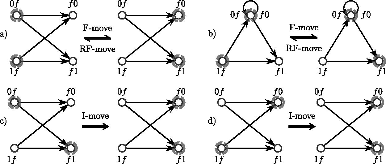
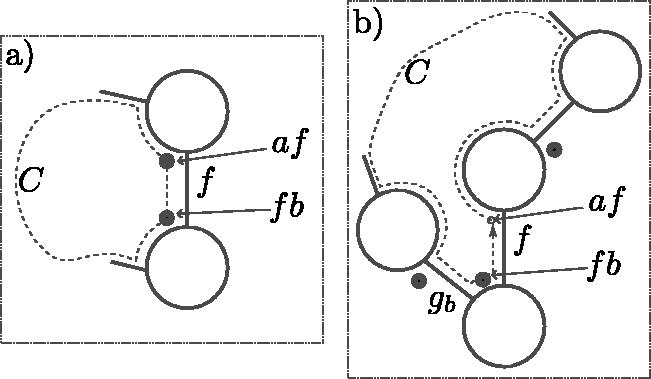
The left-companions (respectively right-companions) is the set of k-mers that have the same suffix (respectively prefix). Given $f\in {\Sigma }^{k-1}$ , then $\mathrm{l}\mathrm{c}(f)\triangleq \left\{af\right|a\in \Sigma \}$ are the left companions sharing the suffix f and $\mathrm{r}\mathrm{c}(f)\triangleq \left\{fa\right|a\in \Sigma \}$ are the right companions. See Figure 1 for examples. If $f=a^{k-1}$ , then the k-mers af and fa are equal (homopolymer a^k), and this k-mer is in both the left- and right-companion sets for f. The homopolymers are the only such k-mers. Every other k-mer is a left companion for exactly one suffix and a right companion for a different prefix.

FIG. 1.

For $f\in {\Sigma }^{k-1}$ , the left-companions (k-mers 0f and 1f for the binary alphabet) and right-companions (f0 and f1) induce a directed complete bipartite $K_{\sigma ,\sigma }$ . (a) When the left-companions are in the set (left subgraph, highlighted in gray), an F-move replaces these nodes with the right-companions (right subgraph). An RF-move is the reverse operation, replacing the right-companions with the left-companions. (b) When one k-mer is a homopolymer (shown here with $f=0^{k-1}$ , so $0f=f0$ ), the induced subgraph is slightly different, but the F-moves and RF-moves are defined analogously. (c) One of the possible I-moves, $f{|}_1$ , where a mixture of left- and right-companions is in the set. (d) The other possible I-move, $f{|}_2$ . For any $f\in {\Sigma }^{k-1}$ there are 1F-move, 1 RF-move, and $2^{\sigma }-2$ I-moves possible, unless f is a homopolymer.

Proposition 1. (Existence of F-moves). In any MDS M, there exists $f,f\prime \in {\Sigma }^{k-1}$ such that M contains the left companions of f and the right companions of $f\prime$ .

Proof. By contradiction, assume that there is no such $f\prime$ . Color all the nodes of the graph blue and do a random walk in the graph, starting from any node not in M, avoiding the nodes in M. Color in red the nodes traversed. Any k-mer m is the left companion of a suffix, say f_m, and every outgoing edge from m is an incoming edge to a right companion of f_m (see Fig. 1). Because no right-companion set is in M, it is always possible to continue the walk avoiding M from any m. Given that the graph is finite, the red nodes will eventually create a cycle, contradicting M being a decycling set. The same reasoning applies for the existence of f traversing edges in the reverse direction.☐

An F-move [named after Fredricksen (1992)] in M for $f\in {\Sigma }^{k-1}$ is the operation of exchanging the set of left companions of f for the set of right companions, as shown in Figure 1. We use the functional notation fM to designate the set obtained by the valid F-move f from M: $fM\triangleq M\cup \mathrm{r}\mathrm{c}(f)\mathrm{\setminus }\mathrm{l}\mathrm{c}(f)$ . This is a valid operation only when M contains lc(f). As a consequence of Proposition 1 there always exists a valid F-move in an MDS. The RF-move (reverse F-move) is the inverse operation, valid when M contains rc(f), $f^{r}M\triangleq M\cup \mathrm{l}\mathrm{c}(f)\mathrm{\setminus }\mathrm{r}\mathrm{c}(f)$ , satisfying $f^{r}fM=f{f}^{r}M=M$ .

Proposition 2. (F-moves preserve decycling sets). Let M be an MDS such that $\mathrm{l}\mathrm{c}(f)\subset M$ , then fM is also an MDS.

Proof. If there is a cycle that avoids fM, then it must use one of the nodes in lc(f), otherwise it was already a cycle avoiding M. Any cycle using a node in lc(f) then must use a node in $\mathrm{r}\mathrm{c}(f)\subset fM$ .☐

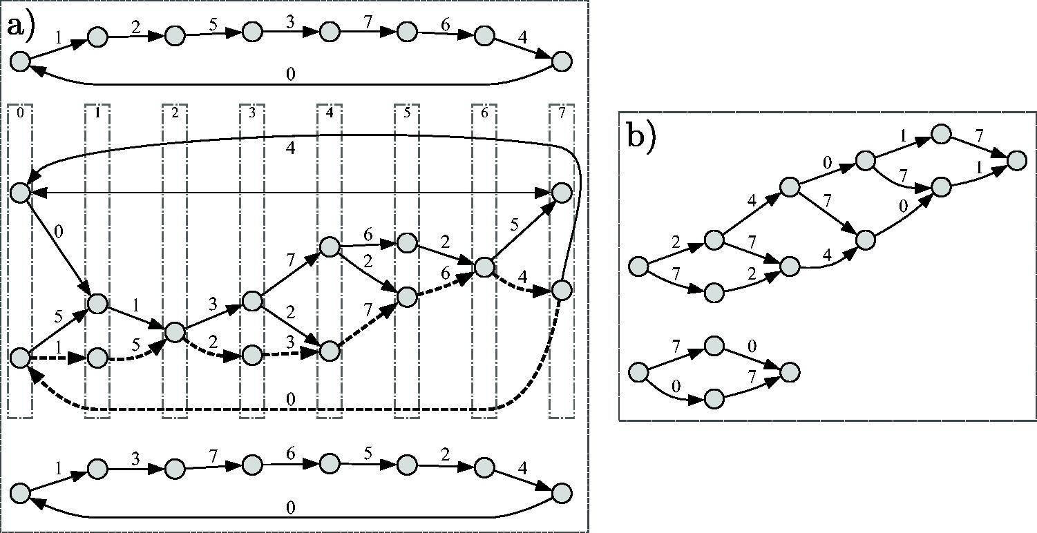
An analogous statement holds for RF-moves. F-moves give a procedure to enumerate some MDSs, starting, for example, from either the Mykkeltveit or Champarnaud set and repeatedly applying a (guaranteed-to-exist by Prop. 1) F-move. Unfortunately, not all MDSs are reachable using only F-moves. The MDS graph $G_{\text{MDS}}(\sigma ,k)$ has all the MDSs as nodes and edges that represent F-moves operations between MDSs. $G_{\text{MDS}}$ is not connected, as seen in Figure 2, but its components have a well characterized structure (proof in Section 8.1).

FIG. 2.

(a) MDS graph $G_{\text{MDS}}(2,4)$ with edge labels as numbers in $[0,{\sigma }^{k-1}]$ representing the F-moves. There are 3 components. Each component is strongly connected and can be partitioned into ${\sigma }^{k-1}=8$ layers with edges only from one layer to the next. The gray vertical boxes in the middle component highlight the layers, numbered from 0 to ${\sigma }^{k-1}$ . Each layer in the middle component has size 1 or 2. An example of a cycle of length 8 with every F-move done exactly once is highlighted with dashed edges. (b) Example of 2 components of nondecycling PCR sets. The components are DAGs with a longest path less than 8 edges.

Proposition 3. ( $G_{\text{MDS}}$ component structure). For any σ and k, the components of $G_{\text{MDS}}(\sigma ,k)$ satisfy the following:

1. 1.

Every component is strongly connected.

The length of every cycle is a multiple of ${\sigma }^{k-1}$ , that is, for every cycle C, there exists ${\alpha }_C\in {\mathbb{N}}^{*}$ such that C is of length ${\alpha }_C{\sigma }^{k-1}$ .

In a cycle of length $\alpha {\sigma }^{k-1}$ , every possible F-move $f\in {\Sigma }^{k-1}$ occurs exactly α times.

Every node is in a cycle of length ${\sigma }^{k-1}$ (hence the girth is ${\sigma }^{k-1}$ ).

Each component is a ${\sigma }^{k-1}$ -partite directed graph.

4.2. I-moves

An I-move, as in an “incomplete F-move,” is valid when M contains a mixture of left- and right-companions: for some $f\in {\Sigma }^{k-1}$ and $\forall a\in \Sigma$ , either af or fa is in M. See Figure 1 for an example. For a given $f\in {\Sigma }^{k-1}$ , there are $2^{\sigma }-2$ distinct I-moves as follows: one for each possible choice of left-companion nodes in M, excluding the F-move [all of lc(f)] and the RF-move [none of lc(f)]. There is one exception as follows: when $f=a^{k-1}$ is a homopolymer, af = fa is both in lc(f) and rc(f), and the number of possible I-moves for f is $2^{\sigma -1}-2$ .

An I-move is denoted by $f{|}_m$ where $m\in [1,2^{\sigma }-2]$ is interpreted as a bit mask giving the nodes from lc(f) (i.e., the ath bit m_a = 1 if $af\in M$ and m_b = 0 if $fb\in M$ ). With this notation, the F-move f would be equivalent to $f{|}_0$ , whereas the RF-move would be $f{|}_{2^{\sigma }-1}$ . By definition the notation $f{|}_m$ implicitly implies that it is a potential I-move and that m is neither the empty nor the full mask ( $m\ne 0$ and $m\ne 2^{\sigma }-1$ ). An identical argument as for Proposition 2 shows that applying a valid I-move to an MDS also gives an MDS.

Although F-moves and I-moves seem like similar operations and both preserve MDSs, they have distinct effect on MDSs. First, empirically we observe that I-moves, unlike F-moves, are not always possible. MDSs always have a valid F-move (Proposition 1), whereas an MDS may not have any valid I-move. All of the ${\sigma }^{k-1}$ F-moves are represented by an edge in every component of the MDS graph. By contrast, out of the ${\sigma }^{k-1}·(2^{\sigma }-2)$ potential I-moves, only a subset of those are valid operations. σ = 2 and k = 5 is an extreme case where no MDS has any valid I-move. Moreover, some I-moves can be a valid operation in one component and not in another.

Second, F-moves not only preserve the decycling property of MDSs, but they also preserve the “coverage” of every cycle by an MDS. To make this notion precise, define the hitting number of a cycle C of D_k by the MDS M as the size of their intersection: ${\mathcal{H}}_M(C)=|M\cap C|$ . Because M is a decycling set, necessarily ${\mathcal{H}}_M(C)\ge 1$ . PCRs, for example, have a hitting number of 1, whereas any Hamiltonian cycle has a hitting number equal to $\left|M\right|$ .

Furthermore, the cycle signature of MDS M is the vector of all hitting numbers for all possible cycles: $\mathcal{S}(M)={〈{\mathcal{H}}_M(C)〉}_{C\text{\hspace{0.17em}cycle\hspace{0.17em}of\hspace{0.17em}}{D}_k}$ . Per the following proposition, F-moves preserve hitting numbers and signatures, whereas I-moves do not.

Proposition 4.

1. 1.

   Let M be an MDS and f a valid F-move in M, then for any cycle C, ${\mathcal{H}}_M(C)={\mathcal{H}}_{fM}(C)$ .

   2.

   For every valid I-move $f{|}_m$ in MDS M, there exists a cycle C of D_k such that ${\mathcal{H}}_M(C)\ne {\mathcal{H}}_{f{|}_{m}M}(C)$ .

   3.

   For any MDS M₁, M₂ from the same component of $G_{\text{MDS}},\mathcal{S}(M_1)=\mathcal{S}(M_2)$ .

   4.

   For any MDS M₁, M₂ from different components of $G_{\text{MDS}},\mathcal{S}(M_1)\ne \mathcal{S}(M_2)$ .

   Proof. Let f be a valid F-move in MDS M and C be a cycle of D_k. Because every outgoing edge of a node in lc(f) is an incoming edge to a node in rc(f), C must contain as many nodes from lc(f) as from rc(f) (which can be 0). Before the F-move, all the nodes from lc(f) and none from rc(f) are in M, whereas the opposite is true for fM. Hence the hitting number is unaffected by the F-move, proving 1.

   Let $f{|}_m$ be a valid I-move in M, $a,b\in \Sigma$ , such that m_a = 1 and m_b = 0 (i.e., both af and fb are in M). Because D_k is $(\sigma -1)$ -vertex connected (Sridhar, 1988), there exists a path P from fb to af  that avoids $cf,c\in \Sigma \mathrm{\setminus }\left\{a\right\}$ . Path P followed by edge $af\to fb$ form a cycle C such that ${\mathcal{H}}_M(C)={\mathcal{H}}_{fM}(C)+1$ (af is in M but not in fM). By the same construction, there exists a “complementary” cycle $C\prime$ using bf and fa such that ${\mathcal{H}}_M(C\prime )={\mathcal{H}}_{fM}(C\prime )-1$ . This proves 2.

   As a component of G_MDS is strongly connected by F-moves, statement 3 is a direct consequence of 1. A proof for 4 is given in Section 8.2.☐

   As a consequence of this proposition, the hitting number and signature are constant over a component of the MDS graph, and the hitting number ${\mathcal{H}}_{\chi }(C)$ and the signature $\mathcal{S}(\chi )$ are well defined for a component χ. Because an I-move changes the signature, every I-move links MDSs from different components. Consider now the component graph $G_{\text{comp}}(\sigma ,k)$ with one node for each component of G_MDS and a directed edge from component ${\chi }_1\to {\chi }_2$ if there is an I-move from an MDS $M_1\in {\chi }_1$ to $M_2\in {\chi }_2$ . In fact, as stated in the following Proposition, G_comp is an undirected graph (proof in Section 8.3).

   Proposition 5. ( $G_{\text{comp}}$ is undirected). Let $f{|}_m$ be a valid I-move from MDS M₁ in component χ₁ to M₂ in χ₂. Then there exists $M{\prime }_2,M{\prime }_1$ in ${\chi }_2,{\chi }_1$ , respectively, such that $f{|}_{\overline{m}}$ (where $\overline{m}$ is the bit-complement of m) is a valid I-move from $M{\prime }_2$ to $M{\prime }_1$ .

   4.3. Enumerating All MDSs

   We make the following two conjectures regarding the use of I-moves to enumerate all MDSs.

   Conjecture 1 (Connectivity by I-moves). The G_comp graph is connected. Equivalently, every MDS is reachable from the Mykkeltveit MDS using a sequence of F-moves and I-moves.

   This conjecture is supported by the previous theoretical results, in particular that all the components have a different signature and that an I-move always changes the signatures. For reasonable values of k (σ = 2, $k\le 7$ ), it is computationally feasible to enumerate all PCR sets and check which of them are also decycling sets. Using this brute force method we can confirm that $G_{\text{comp}}(2,k)$ is connected up to k = 7.

   The following conjecture is computationally also verified up to k = 7 and exposes another fundamental difference between F-moves and I-moves. Every F-move is always valid in every component, whereas the valid I-moves identify a component (similar to the cycle signature). For a component χ, let the list of I-moves be $\mathcal{I}(\chi )=\left\{f{|}_m\right|\exists M\in \chi \text{\&\hspace{0.17em}where\&\hspace{0.17em}}f{|}_m\text{is}\text{a}\text{valid}\text{I-move}\text{in}M\}$ .

   Conjecture 2 (I-move signature). Every component in $G_{\text{MDS}}$ has a distinct list of valid I-moves.

   The validity of this second conjecture is likely related to the previous one. To prove Conjecture 1, one needs to show that for any two components ${\chi }_1,{\chi }_2$ there is a path of I-moves to go from χ₁ to χ₂. Conjecture 2 can be used as a guide to find that path: because $\mathcal{I}({\chi }_1)\ne \mathcal{I}({\chi }_2)$ , then there exists a valid I-move in either $\mathcal{I}({\chi }_1)\mathrm{\setminus }\mathcal{I}({\chi }_2)$ or $\mathcal{I}({\chi }_2)\mathrm{\setminus }\mathcal{I}({\chi }_1)$ (note that it is possible to have, for example, $\mathcal{I}({\chi }_1)\subset \mathcal{I}({\chi }_2)$ ). Do that I-move and repeat with the new components. Although in our testing Conjecture 2 is useful to find a path from χ₁ to χ₂, it is not sufficient as it does not guarantee that the size of the difference between the I-move lists is decreasing.

   To create Table 1 we use both conjectures as follows: one to traverse the graph and the other to avoid enumerating a component more than once. The results in this table empirically show that, independent of the validity of the two preceding conjectures, the space of MDSs reachable using F-moves and I-moves is very large. The ability to traverse that previously unexplored space of MDSs allows us to create optimizing methods to create new sketching methods.

   Table 1.

   G_comp and G_MDS Properties for σ = 2

   Method	Exhaustive						I-moves
   k	2	3	4	5	6	7	8	9	10
   # components	1	1	3	1	273	4	194,133	4,318,173	195,740,496
   # MDSs	2	4	30	28	68,288	18,432	$\approx 3.1·{10}^{11}$	$>1.3·{10}^{17}$	—
   Layer range	1–1	1–1	1–2	1–2	1–48	28–153	$\approx 2.5·{10}^3–29·{10}^3$	$>1.2·{10}^8$	—

   “Layer range” gives, when possible, the range of the number of Minimum Decycling Sets (MDSs) in each layer of G_MDS. The numbers for $k\le 7$ are exact, computed from the exhaustive list of MDSs. For columns $k\in [8,10]$ , the number of components is correct provided the conjectures are correct, otherwise the numbers provided are under-estimations. For k = 8, the layer size and number of MDSs are estimated by sampling 100 random components. For k = 9, the numbers are likely severe under-estimations. For k = 10, computation is too expansive. For the DNA alphabet σ = 4, these numbers would grow even more quickly

4.4. Nondecycling PCR Sets

Nondecycling PCR sets may also have valid F-moves and I-moves, but there are significant differences with MDSs. Unlike MDSs (see Proposition 1), a nondecycling set is not guaranteed to contain sets of left- and right-companions. Even more, the analog graph to G_MDS with nondecycling PCR sets as nodes and F-moves for edges is a nonconnected graph where each component is a DAG (see Fig. 2 and Section 8.4). There cannot be any F-moves between an MDS and a nondecycling set. In contrast, there can be an I-move from a nondecycling set to an MDS (but not the other way around).

5. REMAINING PATH LENGTH AND WINDOW GUARANTEE

By traversing the component graphs and the MDS graph, one can search for MDSs with desirable properties. Unfortunately, as seen in Table 1, every aspect of these graphs (i.e., number of MDS, number of components, layer size, and so on) seems to have super-exponential growth. Enumerating all MDSs for $k\ge 9$ with the binary alphabet is likely not reasonable, and for the DNA alphabet it is even more difficult. In this section, we provide some methods to explore the space of MDSs more efficiently and study the window guarantee of MDSs.

5.1. Efficiently Traversing the Component Graph

As is seen in Table 1, the number of MDSs and components is increasing quickly with k, although an actual estimate of the growth as a function of k is not known. The memory used to traverse a component can be reduced by noticing that each component is partitioned into ${\sigma }^{k-1}$ layers with edges only from one layer to the next (see Fig. 2). Therefore, it is only necessary to keep in memory the MDSs of the current and next layer to exhaustively enumerate every MDS in the component.

As each component contains at least one cycle of length ${\sigma }^{k-1}$ , the number of MDSs grows by at least a factor of ${\sigma }^{k-1}$ faster compared with components. In fact, it grows much faster as each of the ${\sigma }^{k-1}$ layers has a size that grows fast with k as well (see Table 1). While the number of MDSs and the size of the layers varies significantly between components, in general it is not efficient to traverse an entire component to find all the valid I-moves. Using the following proposition, it is possible to find all the valid I-moves in a component by considering only one MDS.

Given an MDS M, any cycle C satisfies $H_M(C)\ge 1$ . The cycles with a hitting number of exactly 1, called constrained cycles, play an important role in the existence or not of a valid I-move: an I-move is only valid if there is no constrained cycle using edges of the I-move.

   Proposition 6. Let $f\in {\Sigma }^{k-1},m\in [1,2^{\sigma }-2]$ , and let χ be a component of $G_{\mathit{MDS}}$ . Then $f{|}_m$ is not a valid I-move in any MDS of χ if and only if $\exists a,b$ such that $m_a=1,m_b=0$ and there exists a constrained cycle using the edge $af\to fb$ .

This proposition, proved in Section 8.5, shows that to find the list of valid I-moves in the entire component it is sufficient to find the edges not covered by a constrained cycle in just one of the MDSs of the component. This holds, as by Proposition 1, that the list of constrained cycles is constant across the MDSs of a component. Moreover, tagging the edges covered by constrained cycle can be done with one depth first search for each k-mer in the MDS. The main advantage of this method is that its run time is independent of the number of MDSs in the component.

5.2. Remaining Path Length

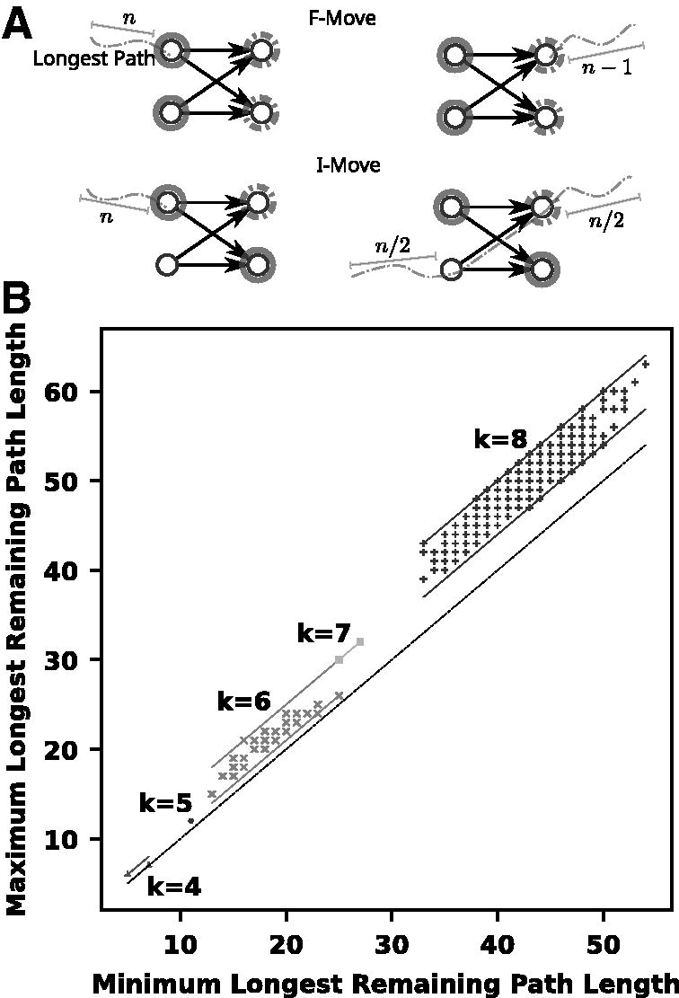
The remaining path length of an MDS, M, is the length of the longest path in the DAG obtained by removing the k-mers of M from D_k. Given a selection scheme that selects in a sequence the k-mers from M, the remaining path length is precisely the window guarantee of the scheme. The following proposition gives bounds on the effect of an F-move or I-move on the remaining path length (see Fig. 3).

FIG. 3.

Left: If a longest path does not start at a valid F-move f, i.e., one of the left-companion of f in solid gray is missing, then it could be extended to the left, contradicting maximality. Doing F-move f (changing solid gray for dashed nodes) can shorten the longest path by 1 node. Also, after doing F-move f, a path now ending in one of the solid gray nodes could be the longest and was extended by 1 node. If the path goes through an I-move $f\prime \prime {|}_m$ , then doing the I-move cuts the path in two possibly equal parts. Right: Comparison of the minimum and maximum remaining longest path for components of $G_{\text{MDS}}(2,k)$ for $4\le k\le 8$ . Each point represents one connected component of the graph. The minimum and maximum remaining path lengths are computed over all the MDSs of a component. Therefore, the vertical distance of a point from the diagonal y = x (in yellow) shows the variation of remaining path length within a component. For k = 8, a subsample of 500 components was examined, as the total number of components is exceedingly large. The lines are drawn to depict the bounds of the increase between components. In all cases seen, the difference between the minimum and maximum remaining length within a component is in some range $[\alpha ,\alpha +k]$ for an alpha that is less than k.

Proposition 7. An F-move or RF-move can increase or decrease the remaining path length by at most 1. An I-move can increase the remaining path length by at most 1 or decrease it by at most half.

Proof. First, notice that the longest path in $D_k\mathrm{\setminus }M$ must start at a valid F-move and end at a valid RF-move. Let $P=(m_1,\dots ,m_n)$ be a longest path. The k-mer m₁ is the right companion of some suffix f. Suppose there exists $a\in \Sigma$ such that $af\notin M$ , then the path $P\prime =(af,m_1,\dots ,m_n)$ avoids M and is longer than P, contradicting its maximality. Therefore $\mathrm{l}\mathrm{c}(f)\subset M$ and f is a valid F-move in M. The proof is symmetrical for m_n as the left-companion of some prefix $f\prime$ with $rc(f\prime )\subset M$ .

Because $m_1\in fM$ , the path P is shortened by 1 by the F-move f, which may shorten the longest path if there were no other paths of that length. In addition, $rc(f)\subset fM$ (i.e., f is a valid RF-move in fM but it was not in M); hence, there might be maximal path $P\prime$ ending at a left-companion of f with $|P\prime |>n$ . Because the F-move only moved nodes forward by one edge, $|P\prime |\le n+1$ and the longest path may have increased by 1. The same argument applies to an RF-move.

For a valid I-move $f\prime \prime {|}_m$ in M, the same reasoning applies for increasing by 1. In contrast, a longest path may have used an edge $af\prime \prime \to f\prime \prime b$ where $m_a=0,m_b=1$ . That is, $P=(m_1,\dots ,m_i=af\prime \prime ,m_{i+1}=f\prime \prime b,\dots ,m_n)$ . After the I-move, $fb\in f\prime \prime {|}_{m}M$ , and the path is now broken in up to two parts as follows: $(m_1,\dots ,m_i)$ and $(m_{i+2},\dots ,m_n)$ . Therefore, the remaining path length could be halved if $i=n/2$ . ☐

Based on this, we implemented a simulated annealing algorithm to find the smallest and largest remaining path lengths among MDSs. The longest path for the MDS M is computed using a modified topological sort of the DAG $D_k\mathrm{\setminus }M$ . Suppose that we are computing the smallest remaining path length. Starting from a component of the MDS graph, the program performs a fixed number of random F-moves (2k by default) and computes the remaining path length for each MDS and keeps the minimum. Then, it finds all the valid I-moves in the current component as explained in Section 5.1, and it picks one at random.

After performing the I-move, in the new component, the remaining path length is computed for 2k MDSs reachable by F-moves and a new minimum is computed. If this new minimum is lower than the previous minimum, then the new component becomes the current component. Otherwise, it becomes the current component only with some small probability. Then the process is repeated from the current component for a fixed number of iterations. As is traditional with simulated annealing, the probability to jump to “worse” components decreases over time.

Table 2 shows the remaining path length for the two previously known algorithms to generate MDSs and the range of remaining path length. These ranges are either exact when an exhaustive list of MDSs is computable and approximated using simulated annealing otherwise. Based on the pattern that the Mykkeltveit set is always at or close to the minimum remaining path length, we conjecture that it holds for all parameters k and σ.

Table 2.

The Remaining Path Length for the Mykkeltveit and Champarnaud Sets Compared With the Range of Remaining Path Length

σ	Algorithm	k
		4	5	6	7	8	9	10	11	12	13	14	15	16	17	18	19	20
		2	Mykkeltveit	5	11	21	27	39	55	74	89	119	143	194	219	253	299	408	437	539
	Champarnaud	7	11	21	27	47	57	94	112	190	209	367	415	683	756	1343	1393	2560
	SA Min	5	11	13	25	32	48	70	89	119	143	194
	SA Max	7	12	26	32	55	80	116	158	257	288	387
4	Mykkeltveit	21	41	77	111	145	231	330	403	616
	Champarnaud	27	39	119	141	429	520	1601	1765	6180
	SA Min	20	41	77	111	145
	SA Max	34	66	149	270	530

For σ = 2 and $k\le 7$ , the range of remaining path length is computed exactly from the exhaustive list of MDSs. The other values in the simulated annealing (SA) Min and SA Max rows are estimated using an SA algorithm and are underlined.

Conjecture 3. For a given σ, let ${\ell }_{\text{min}}(k),{\ell }_{\text{max}}(k),{\ell }_{\text{Mykk}}(k)$ , respectively, be the smallest, largest, and Mykkeltveit set remaining path lengths. Then ${\ell }_{\text{Mykk}}(k)-{\ell }_{\text{min}}(k)=o({\ell }_{\text{max}}(k)-{\ell }_{\text{min}}(k))$ asymptotically in k.

5.3. Per-Component Remaining Path Length

Proposition 7 gives a bound on the change in the remaining path length as the MDS graph is traversed using F-moves and I-moves. Within one component, given that every MDS is in a cycle of length σ^k, the remaining path length along this cycle could change by up to ${\sigma }^k/2$ . In other words, this proposition only gives an exponential bound on the range of remaining path length within a component.

The graph in Figure 3 has a point for each component at the coordinate $(m_P(\chi ),M_P(\chi ))$ where $m_P(\chi )$ is the minimum of the remaining path length over all the MDSs of the component χ, and $M_P(\chi )$ is the maximum. The vertical distance from the diagonal y = x represents the range of remaining path lengths within a component. We observe for $k\le 8$ on the binary alphabet that the range is bounded by O(k).

Conjecture 4. Within a component of G_MDS, the range of remaining path length is O(k).

There are plausible reasons for having such a small range. Consider the following two extremes: (1) there are many F-moves and RF-moves valid at the same time in an MDS M, (2) there is only 1 F-move and 1 RF-move valid in M. In the first case, doing one of these F-moves or RF-moves affects the maximal paths that start or end at these moves. Consequently, many of these moves change the length of paths that are not the longest. In other words, these moves have no effect on the remaining path length. In the second case, it is possible to show that doing the 1 valid F-move does not change the remaining path length (the longest path is truncated by its first node and extending by one node, hence not changing in length). This type of situation is likely to happen when there are few F-moves and RF-moves possible. In both cases, most F-moves do not affect the remaining path length.

This conjecture partially justifies only exploring O(k) MDSs within one component in the simulated annealing algorithm in Section 5.2.

6. DISCUSSION

Proportion of MDSs. A simple algorithm to generate a random MDS, sampling the space of MDSs uniformly, is to select at random k-mer from each PCR and check whether it is decycling, and to resample if not. Even though the space of MDSs is (maybe surprisingly) large, it is nonetheless only a tiny fraction of the PCR sets. The number of PCR sets is easily computable (Fredricksen and Kessler, 1986), and asymptotically, there are $\Omega (k^{{\sigma }^k/k})$ PCR sets. There is no formula for the number of MDSs, but based on the numbers from Table 1, for k = 8, of the $2·{10}^{29}$ PCR sets the proportion that are MDSs is only $2·{10}^{-18}$ . For k = 9 that proportion is essentially 0. Thus, the random sampling method is not of any practical use.

In that sense Conjecture 1, provided it is true, is an efficient method to enumerate all MDSs as only MDSs are ever considered without the need to filter out an overwhelming number of nondecycling sets. Even if this conjecture is eventually proven wrong, the F-moves and I-moves allow us to explore a large subspace of MDSs and, using simulated annealing or more advanced machine learning methods, to find MDSs with desirable properties.

Moreover, on the theoretical side, providing evidence for this conjecture lead us to a deeper understanding of the space of MDSs and to formulate the other conjectures.

Mykkeltveit set and short windows. It is surprising (or lucky) that the first algorithm for constructing MDSs by Mykkeltveit (1972) gives a set with close to the shortest remaining path length. This fact may explain retrospectively the success of previous methods using this set as the starting point to design minimizers schemes (Orenstein et al., 2016, 2017; Ekim et al., 2020; Pellow et al., 2023). The growth of the remaining path length for the Mykkeltveit set is well characterized (Zheng et al., 2020a): it is $\Omega (k^2)$ and $O(k^3)$ . Fitting the data from Table 2 we obtain an exponent of 3.12 ± 0.14, suggesting an actual growth of $\Theta (k^3)$ . Provided that Conjecture 3 holds, this would answer the question of the shortest window guarantee that is possible using an MDS. For comparison, fitting the Champarnaud data gives an exponent of 6.1 ± 0.59.

Longest remaining path length. Conjecture 4 only suggests a bound on the range of remaining path length within a component of G_MDS. A legitimate question is what is the bound of the range in G_MDS as a whole. Figure 3 could suggest that this range is polynomial in k, although the trend in this figure is much too short to elevate this statement to a conjecture. Given the known results bounding the longest remaining path of the Mykkeltveit set by $O(k^3)$ , this would mean a polynomial bound on the remaining path length of MDSs.

This statement seems counterintuitive at first (and is, of course, not proven). We saw in Section 3 that syncmers have a window guarantee of ${\sigma }^{k-1}$ ; hence, there exists DSs that are not of minimum size that have exponentially long remaining paths. How then can sets with fewer k-mers (MDSs) have a shorter remaining path length? The intuition is as follows. In the syncmers construction, we chose one exponentially long path (length ${\sigma }^{k-1}-1$ ) through the graph, whereas every node not on this path is added to the DS M. The size of the DS $\left|M\right|={\sigma }^k(1-1/\sigma )$ is exponential as well: it takes many nodes, guiding that long path, to prevent cycles. In contrast, the size of an MDS is $\sim {\sigma }^k/k$ , which is $o({\sigma }^k)$ . The average remaining path length is k and there are too few k-mers in an MDS to guide an exponentially long path to prevent it from creating cycles (i.e., to have back edges).

In practice, even a $O(k^3)$ window guarantee may be too long, and an MDS may need to be extended to a decycling set with even shorter remaining path length [as done in Orenstein et al. (2017)]. Hence starting with an MDS with the shortest possible remaining path length is advantageous. Even if Conjecture 3 is true, it does not prevent the existence of decycling sets with smaller remaining path lengths than the Mykkeltveit set. Whether MDSs with remaining path length of $o(k^3)$ exist is still an open question.

7. CONCLUSION

The window guarantee is an important requirement, theoretically and practically, to define and optimize sketching methods. As discussed, an underlying concept that can be extracted from the definition of this guarantee in any local sketching method is a set of nodes in the de Bruijn graph which are unavoidable (i.e., decycling). While many such sets exist, the minimum-sized sets have important properties that can be exploited and examined. In this work, we described some of the first theoretical findings on properties of these sets, as well as a method to traverse many (if perhaps not all) MDSs for a given k-mer length. We also showed that the choice of MDS, whether direct or as an implication of the design of the sketching method, does have an impact on the strength of the window guarantee. Although we provide our major results as conjectures, we present significant evidence to support these claims.

8. EXTENDED PROOFS

8.1. MDS Graph Structure

Lemma 1 (Commutative property). Let M be an MDS and $f_1,f_2\in {\Sigma }^{k-1}$ be two valid F-moves in M, then f₁ is a valid F-move in $f_{2}M$ , f₂ is valid in $f_{1}M$ , and $f_1{f}_{2}M=f_2{f}_{1}M$ .

Proof. The left companions of f₁ and f₂ are all in different PCRs. Hence, after doing the F-move f₁ or f₂, the other F-move is still valid. Moreover, regardless of the order in which the F-moves are performed, the resulting set is the same.

There is no equivalent statement to Lemma 1 for I-moves: if $f_1{|}_{m_1},f_2{|}_{m_2}$ are two valid I-moves in M, then $f_2{|}_{m_2}$ may not be valid in $f_1{|}_{m_1}M$ .

Lemma 1 applies to a sequence of F-moves $(f_1,\dots ,f_{i-1},f_i,f_{i+1},\dots ,f_n)$ . Suppose that this is a valid sequence of F-moves starting from MDS M and that both f_i and $f_{i+1}$ are valid F-moves in $f_{i-1}\dots f_{1}M$ , then $f_{i+1}{f}_i{f}_{i-1}\dots f_{1}M=f_i{f}_{i+1}{f}_{i-1}\dots f_{1}M$ and $f_n\dots f_{i+1}{f}_i{f}_{i-1}\dots f_{1}M=f_n\dots f_i{f}_{i+1}{f}_{i-1}\dots f_{1}M$ .

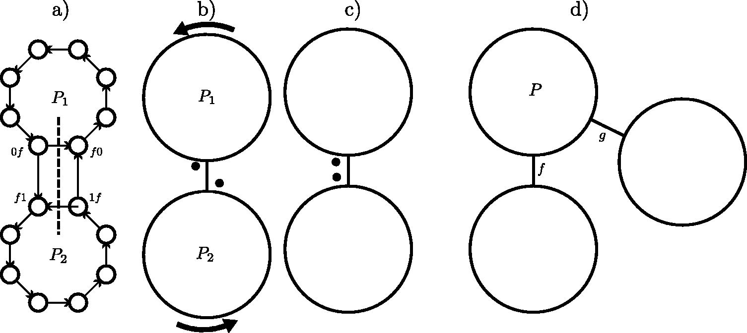
In the following proofs, we use the simplified representation for PCRs, F- and I-moves given in Figure 4. For simplicity, the figure shows an example with the binary alphabet. When $\sigma >2$ , an F-move f represents a hyperedge between σ PCRs rather than a simple edge as shown.

FIG. 4.

Simplified representation of PCRs, F-moves, and I-moves when σ = 2. (a) shows two PCRs from the de Bruijn graph D_k. Every PCR is a circle, and they are all oriented counterclockwise (see PCR P₁ and P₂ here). Let f be an F-move that involves P₁, P₂. Here P₁ has the edge $0f\to f0$ , and P₂ has $1f\to f1$ : these are the PCR edges. The cross-PCR edges $0f\to f1$ and $1f\to f0$ form antiparallel edges between P₁ and P₂. (b) The simplified PCR/pebbles representation shows PCRs as large cycles without representing individual k-mers and only representing the F-move edges of interest. The elements from the MDS in each PCR (the pebbles) are small black circles that can travel only counterclockwise around the PCR. An F-move is an edge between P₁ and P₂ and acts as a semaphore: a pebble can move one step around the PCR and across the edge of f only when the other pebbles are present next to the edge in the other PCR [i.e., lc(f) is in the MDS], as shown in b), and all pebbles move across the edge at the same time. (c) The position of the pebbles for the I-move $f{|}_1$ : bit 0 is set but not bit 1, so the pebbles are on 0f and f1 (left side of the edge of f). The top pebble can move across the edge, counterclockwise, whereas the lower one stays still. For I-move $f{|}_2$ with bit 0 unset and bit 1 set, the pebbles would be on 1f and f0, on the right side of the edge of f. (d) If F-moves f and g have a PCR P in common, then, because F-moves act like semaphores, it is not possible to do the F-move f twice before g is done once. For the pebble to go around P to do f a second time, necessarily the F-move g was done as well. PCR, pure cycling register.

Proposition 3. ( $G_{\text{MDS}}$ component structure). For any σ and k, the components of $G_{\text{MDS}}(\sigma ,k)$ satisfy the following:

1. 1.

Every component is strongly connected.

2.

The length of every cycle is a multiple of ${\sigma }^{k-1}$ , that is, for every cycle C, there exists ${\alpha }_C\in {\mathbb{N}}^{*}$ such that C is of length ${\alpha }_C{\sigma }^{k-1}$ .

3.

In a cycle of length $\alpha {\sigma }^{k-1}$ , every possible F-move $f\in {\Sigma }^{k-1}$ occurs exactly α times.

4.

Every node is in a cycle of length ${\sigma }^{k-1}$ (hence the girth is ${\sigma }^{k-1}$ ).

5.

Each component is a ${\sigma }^{k-1}$ -partite directed graph.

Proof of points 2 and 3, length of cycles. Every PCR is a cycle in D_k, and an MDS M is seen as pebbles sitting on the k-mers (see Fig. 4b). There is one pebble per PCR. An F-move involves σ distinct PCRs (edges $af\to fa,a\in \Sigma$ are each in their own PCR). Hence, an F-move is a hyperedge connecting σ PCRs. An F-move is like moving the pebbles along σ PCRs at a time, from left-companions to right-companions, and this move is legal only if $\mathrm{l}\mathrm{c}(f)\subset M$ . In that sense, an F-move is like a semaphore: pebbles can move only if all their left-companions are present in the set.

First, because every MDS has a valid F-move and a component of G_MDS is finite, a component must have a cycle. Let $C=(M_0,\dots ,M_{n-1})$ be a cycle of MDSs in G_MDS, and equivalently $C=(f_0,\dots ,f_{n-1})$ is a list of F-moves such that $M_{i+1}=f_i{M}_i$ (indices taken modulo n). After doing F-move f₀, the pebble on at least one PCR, say P₀, has moved. Because C is a cycle, by the time $f_{n-1}$ is done, all pebbles are back on their respective starting spot. Meaning the pebble on P₀ went all the way around (possibly multiple times) P₀. To move around P₀ with F-moves, the pebbles in the PCRs adjacent to P₀ must have moved as well. By the time $f_{n-1}$ is done, every pebble in the PCRs adjacent to P₀ has moved around its respective PCR. By transitivity, and because the de Bruijn graph is strongly connected, every pebble on every PCR has gone around its PCR after $f_{n-1}$ is done. Because every pebble went around its PCR, this means that every one of the ${\sigma }^{k-1}$ F-moves was done and $n\ge {\sigma }^{k-1}$ .

Conversely, because the F-move/hyperedge act as semaphores, it is not possible for a pebble on a PCR to do more rotations around its own PCR than the pebbles on the adjacent (by hyperedge) PCRs. To see this, consider the starting position of the pebble on PCR P₀. For this pebble to start a second turn around P₀, all of its left-companions must be back on their starting spot and also start a second turn around their own PCRs. This holds for all PCRs by transitivity.

Hence, in a cycle of the MDS graph, the pebbles of all PCRs go around the same number of times, say α, and the number of F-moves in the cycle C is $n=\alpha {\sigma }^{k-1}$ .☐

Proof of point 1, strongly connected. As in the previous proof, there exists a cycle $C=(M_0,\dots ,M_{n-1})$ in G_MDS, and its edges are $(f_0,\dots ,f_{n-1})$ with $M_{i+1}=f_i{M}_i$ .

We show that for any node M_i of this cycle and any neighbor M of M_i, reachable by an F-move or RF-move from M_i, M and M_i are in a cycle. If this holds, by transitivity of the relation “being in the same strongly-connected component”, any pair of nodes in the component are in a cycle and the component is strongly connected.

Without loss of generality, we prove this property for the neighbors of M₀ (see Fig. 5). It is a consequence of the commutativity of the F-moves (Lemma 1). Let $M=f{M}_0$ be a neighbor of M₀ for some $f\ne f_0$ . Because in a cycle all F-moves occur, there exists a first $j\in [1,n-1]$ such that $f_j=f$ (and $f\ne f_i,i\in [0,j-1]$ ). f is valid in M₀; hence, it is also valid in M₁, and recursively in $M_2,\dots ,M_j$ . Therefore, f commutes with $f_0,\dots ,f_{j-1}$ , and the sequence of F-move $(f_j,f_0,\dots ,f_{j-1})$ is another path from M₀ to $M_{j+1}$ that is going through M. This path followed by the remainder of C from $M_{j+1}$ back to M₀ is a cycle that includes both M₀ and M.☐

FIG. 5.

Example of a cycle in $G_{\text{MDS}}(2,4)$ . The outer circle is $C=(f_0,\dots ,f_7)$ , a cycle of length ${\sigma }^{k-1}$ . $M=f{M}_0$ is a neighbor of M₀ not on C. Because f must occur in C, here $f=f_3$ , then f commutes with $f_0,f_1,f_2$ . Hence $(f=f_3,f_0,f_1,f_2,f_4,\dots ,f_7)$ is also a cycle in $G_{\text{MDS}}(2,4)$ , and it contains M₀ and M.

Proof of point 4, cycle length ${\sigma }^{k-1}$ . Let M be a MDS on a cycle C in G_MDS. It is of length $\alpha ·{\sigma }^{k-1}$ , with $\alpha \ge 1$ by point 2. Suppose that $\alpha >1$ . Let $C=(f_1,\dots ,f_{\alpha ·{\sigma }^{k-1}})$ be the sequence of F-moves representing that cycle. Every distinct F-move occurs exactly α times in that sequence. We show that the sequence can be reordered so that the ${\sigma }^{k-1}$ different F-moves occur at the first ${\sigma }^{k-1}$ positions of the sequence.

If it is not already the case that the first ${\sigma }^{k-1}$ F-moves are distinct, there must be an F-move f that occurs twice in the list before an F-move g occurs for the first time. Let i < j be two indices which are the first two occurrences of f in the sequence (i.e., $f_i=f_j=f$ ) and such that j + 1 is the first occurrence of g ( $f_{j+1}=g$ ). If any of the PCRs involved in the F-move f are also involved in the F-move g, then it is not possible to use f twice in C before using g (see Fig. 4d). Therefore the PCRs involved in the F-moves f and g are distinct, and g must be a valid F-move just before the second use of f as well. In other words, f_j and $f_{j+1}$ commute.

Repeated swapping of F-moves leads to the desired sequence of F-moves with all ${\sigma }^{k-1}$ distinct F-moves in the first positions, which induces a cycle of length ${\sigma }^{k-1}$ containing M.☐

Proof of point 5, ${\sigma }^{k-1}$ -partite. Partition the nodes of a component of G_MDS as follows. We create ${\sigma }^{k-1}$ sets: ${\mathcal{P}}_0,\dots ,{\mathcal{P}}_{{\sigma }^{k-1}-1}$ . Let M₀ be an arbitrary MDS of the component and assign it to the set ${\mathcal{P}}_0$ . For every other MDS M, take a shortest path $P(M)=M_0\to M$ in G_MDS. Assign M to the partition with index $\left|P\right|\mathrm{mod}{\sigma }^{k-1}$ .

Because M₀ is in a cycle of length ${\sigma }^{k-1}$ , every set ${\mathcal{P}}_i$ has at least one MDS assigned to it. Moreover, every MDS is assigned to exactly one set. Hence the sets ${\mathcal{P}}_i$ form a partition of the MDSs in the component.

An edge between MDSs in sets ${\mathcal{P}}_i$ and ${\mathcal{P}}_j$ with $j>i+1$ would imply the existence of a cycle containing M₀ of length $<{\sigma }^{k-1}$ , which is not possible.☐

8.2. Cycle Signature Is Unique per Component

An MDS M is called f-terminal if the only valid F-move in M is f.

Lemma 2. For any $f\in {\Sigma }^{k-1}$ and in any component of G_MDS, there exists an f-terminal MDS.

Proof. From Proposition 3, in any component there exists an MDS $M\prime$ where f is a valid F-move. If there exists other valid F-moves than f in $M\prime$ , do them recursively. That is, we do every possible F-move in $M\prime$ but refuse to do f. This creates a path P of MDSs in G_MDS starting at $M\prime$ that does not contain f as an edge.

Because every cycle in G_MDS contains every possible F-move, P cannot induce a cycle, and it must terminate at an MDS M. By construction M is f-terminal.☐

An f-terminal MDS M has a useful property: every maximal path in D_k that avoids M (as created by a walk like in Proposition 1) must start at a k-mer $m\in rc(f)$ . Equivalently, any walk in D_k that avoids M following edges backward ends at some $m\in rc(f)$ .

Proposition 4.

1.

Let M be an MDS and f a valid F-move in M, then for any cycle C, ${\mathcal{H}}_M(C)={\mathcal{H}}_{fM}(C)$ .

2.

For every valid I-move $f{|}_m$ in MDS M, there exists a cycle C of D_k such that ${\mathcal{H}}_M(C)\ne {\mathcal{H}}_{f{|}_{m}M}(C)$ .

3.

For any MDS M₁, M₂ from the same component of $G_{\text{MDS}},\mathcal{S}(M_1)=\mathcal{S}(M_2)$ .

4.

For any MDS M₁, M₂ from different components of $G_{\text{MDS}},\mathcal{S}(M_1)\ne \mathcal{S}(M_2)$ .

Points 1–3 were proven in Section 4.2.

Proof of point 4, different signatures. Fix $f\in {\Sigma }^{k-1}$ . Because the signature is constant in a component by point 1, and because by Lemma 2 there always exists an f-terminal MDS in a component, it suffices to show that the signatures are different for two f-terminal MDSs M₁, M₂ from different components. We will construct a cycle C in D_k that has different hitting numbers between the components: ${\mathcal{H}}_{M_1}(C)\ne {\mathcal{H}}_{M_2}(C)$ .

M₁ and M₂ are in different components, so they are distinct MDSs and there exists a PCR R where the selected k-mer is different. That is, $R\cap M_1\triangleq m_1\ne m_2\triangleq R\cap M_2$ . Take a path P in D_k following edges backward from node 0f (which is in both M₁ and M₂ because they are f-terminal) to m₁ that avoids nodes $af,a\in \Sigma \mathrm{\setminus }\left\{0\right\}$ . Path P exists because D_k is $(\sigma -1)$ -connected. Because $m_1\in M_1\Delta M_2$ , there must exist a first node $m\in P$ which is in $M_1\Delta M_2$ .

Let P₁ be the restriction of the path P from 0f to m and, without loss of generality, assume that $m\in M_1$ . By construction, $|P_1\cap M_1|=|P_1\cap M_2|+1$ .

Let P₂ be a path created by a maximal random walk in D_k, following edges backward, starting from m and that avoids M₂. Because M₂ is f-terminal, the walk ends at a node $fa\in rc(f),a\in \Sigma$ . By construction, $|P_2\cap M_1|\ge |P_2\cap M_2|=0$ (P₂ avoids nodes from M₂ but may contain nodes from M₁).

Two cases can happen. First case, there exists a first node $m\prime \in P_1\cap P_2$ . Then define the cycle C as the restriction of P₁ from $m\prime$ to m followed by the restriction of P₂ from m to $m\prime$ . Second case, $P_1\cap P_2=\varnothing$ and define the cycle C as the concatenation of P₁, P₂ and backward edge $fa\to 0f$ .

In both cases, C satisfies by construction ${\mathcal{H}}_{M_1}(C)>{\mathcal{H}}_{M_2}(C)$ .☐

8.3. G_comp Is Undirected

Proposition 5. ( $G_{\text{comp}}$ is undirected). Let $f{|}_m$ be a valid I-move from MDS M₁ in component χ₁ to M₂ in χ₂. Then there exists $M{\prime }_2,M{\prime }_1$ in ${\chi }_2,{\chi }_1$ , respectively, such that $f{|}_{\overline{m}}$ (where $\overline{m}$ is the bit-complement of m) is a valid I-move from $M{\prime }_2$ to $M{\prime }_1$ .

Proof. See Figure 6. In component χ₁, by Proposition 3, there is a cycle C₁ of length ${\sigma }^{k-1}$ that contains MDS M₁, and this cycle has f that has an F-move. Hence, $C_1=(M_1,\dots ,M_1^f,M{\prime }_1,\dots ,M_{{\sigma }^{k-1}})$ , where $M_1^f$ is the MDS where f is a valid I-move and $M{\prime }_1=f{M}_1^f$ . Equivalently, looking at the edges, $C_1=(F_{\overline{m}},f,F_m)$ , where $F_{\overline{m}},F_m$ are sequences of F-moves.

FIG. 6.

Simplified example for finding the complementary I-moves, when σ = 2. On the left box, component χ₁ and component χ₂ on the right of G_MDS. The cycles C₁, C₂ are cycles in χ₁ and χ₂, respectively. The simplified PCR/pebble drawings represent the position of the pebbles on the PCRs of P_m (top PCR) and $P_{\overline{m}}$ (bottom PCR). The edge between these PCRs represents f. The PCR/pebbles drawings next to the MDS nodes represent the state of the PCRs for these MDSs, whereas the drawings next to the dotted line (sequences of F-moves) represent the action of the sequence of F-moves on the pebbles. From the cycle C₁ in χ₁, we construct cycle C₂ in χ₂ by swapping the order of the F-moves: $(F_{\overline{m}},f,F_m)\to (F_m,f,F_{\overline{m}})$ . These cycles go through the desired MDSs $M{\prime }_2$ and $M{\prime }_1$ that are linked by the complementary I-move $f{|}_{\overline{m}}$ .

By hypothesis $f{|}_m$ is a valid I-move in M₁, which means that if m_a = 1, then $af\in M_1$ and $fa\in M_1$ otherwise.

Let’s call P_m the set of PCRs that contain af when m_a = 1 and $P_{\overline{m}}$ the PCRs containing af when m_a = 0 (P_m contains only the top PCR in Fig. 6 and $P_{\overline{m}}$ the bottom PCR).

In $M_1^f$ , f is a valid F-move, which means that $af\in M_1^f$ for all $a\in \Sigma$ . In other words, the sequence of F-moves $F_{\overline{m}}$ made by the pebbles in the PCRs in $P_{\overline{m}}$ goes around from fa to af, whereas the pebbles in the PCRs in P_m did not move. (The only way for the pebbles in the PCRs in P_m to move is to do F-move f, which by construction is not in $F_{\overline{m}}$ ).

Similarly, the sequence of F-moves F_m made by the pebbles in the PCRs in P_m goes around from fa to af, whereas the pebbles in the PCRs of $P_{\overline{m}}$ did not move.

Now from M₁ do the valid I-move $f{|}_m$ . This advances the pebbles in the PCRs of P_m from af to fa (forward by 1 edge), to get to M₂ in component χ₂, where $rc(f)\subset M_2$ . The position of the pebbles in M₁ and M₂ agrees everywhere except on the PCRs of P_m. Because the F-moves in $F_{\overline{m}}$ do not affect the PCRs of P_m, the sequence $F_{\overline{m}}$ is a valid sequence of F-moves in M₂ as well.

$fa\in M_2$ for all $a\in \Sigma$ . Applying $F_{\overline{m}}$ to M₂ leads to MDS $M{\prime }_2$ where $af\in M{\prime }_2$ if m_a = 0 and $fa\in M{\prime }_2$ otherwise. In other words, I-move $f{|}_{\overline{m}}$ is valid in $M{\prime }_2$ . It is easy to check that doing the I-move $f{|}_{\overline{m}}$ gets back to $M{\prime }_1$ .

For completion, one can check that the sequence of F-moves F_m applies to $M{\prime }_2$ because $M{\prime }_2$ and $M{\prime }_1$ only differ on the pebbles on the PCRs of $P_{\overline{m}}$ and F_m does not affect those PCRs. Applying F_m to get to $M_2^f$ where f is a valid F-move and $M_2=f{M}_2^f$ .

Therefore, the cycle $C_1=(F_{\overline{m}},f,F_m)$ is a valid cycle in χ₁ and contains M₁ and $M{\prime }_1$ , whereas $C_2=(F_m,f,F_{\overline{m}})$ is valid in χ₂ and contains M₂ and $M{\prime }_2$ .☐

8.4. Nondecycling PCR Sets

Proposition 8. Let G_PCR be the graph with nondecycling PCR sets as nodes and F-moves as edges. Then each component of G is a DAG.

Proof. Suppose there exists a cycle $\mathcal{C}=\{M_1,\dots ,M_n\}$ in G_PCR, where $M_{i+1}=f_i{M}_i$ . Because M₁ is not decycling, then there exists a cycle C in $D_k\mathrm{\setminus }{M}_1$ . Because RF-moves preserve the hitting number, C is also a cycle in $D_k\mathrm{\setminus }{f}_1{M}_1$ , and by induction a cycle in $D_k\mathrm{\setminus }{M}_i,i\in [1,n]$ . From the proof Proposition 3, any cycle $\mathcal{C}$ must do every ${\sigma }^{k-1}$ F-move to return to the starting set, and the union of all the left-companions of the F-moves is the set of all k-mers. This is a contradiction.☐

8.5. I-moves and Constrained Cycles

Proposition 6. Let $f\in {\Sigma }^{k-1},m\in [1,2^{\sigma }-2]$ , and let χ be a component of $G_{\text{MDS}}$ . Then $f{|}_m$ is not a valid I-move in any MDS of χ if and only if $\exists a,b$ such that $m_a=1,m_b=0$ , and there exists a constrained cycle using the edge $af\to fb$ .

Proof. Let $f{|}_m$ be a potential I-move with m_a = 1 and m_b = 0 ( $a,b\in \Sigma ,a\ne b$ ).

Suppose there exists a constrained cycle C in the de Bruijn graph D_k using the edge $af\to fb$ and $H_{\chi }(C)=1$ . If $f{|}_m$ is a valid I-move in an MDS $M\in \chi$ , then by definition $af,fb\in M$ , hence $H_M(C)\ge 2$ . This contradicts that C is constrained (see Fig. 7a).

FIG. 7.

A) The $f{|}_m$ with m_a = 1 and m_b = 0 is not possible because ${\mathcal{H}}_M(C)=1$ . When the I-move $f{|}_m$ is valid, necessarily C’s hitting number must be at least 2. B) Suppose $f{|}_m$ is never valid, then a backward walk creates a cycle with hitting number 1 using the edge $af\to fb$ .

Conversely, suppose that $f{|}_m$ is not a valid I-move in any MDS of χ. Let $M^f\in \chi$ be an MDS where f is a valid F-move and $M=f{M}^f$ . Then $rc(f)\subset M$ . Define $g_c\triangleq f[2:k-2]c,c\in \Sigma$ , that is, for all right-companion of f, $fc\in \mathrm{l}\mathrm{c}(g_c)$ .

From M recursively do all valid F-moves except for the F-moves g_c where m_c = 0 to obtain $M\prime \in \chi$ where the only valid F-moves are exactly those that we refused to do. There must exist $a\in \Sigma$ such that m_a = 1 and $af\notin M\prime$ , otherwise $f{|}_m$ is a valid I-move in $M\prime$ (see Fig. 7b). From af do a walk that avoids $M\prime$ using backward edges. This walk must end at one of the right-companions of the valid F-moves in $M\prime$ , that is, there exists b such that walk ends at $m\prime \in rc(g_b)$ . By construction there is a backward edge $m\prime \to fb$ . Then follow the backward edge $fb\to af$ to create a cycle C. By construction the only node from $M\prime$ in cycle C is fb, hence ${\mathcal{H}}_{M\prime }(C)=1$ and C uses the edge $af\to fb$ with m_a = 1 and m_b = 0.☐

References

1.
ChamparnaudJ-M, HanselG, PerrinD. Unavoidable sets of constant length. Int J Algebra Comput, 2004; 14(02):241–251; doi: 10.1142/S0218196704001700
2.
DeBlasioD, GbosiboF, KingsfordC, et al.Practical universal k-mer sets for minimizer schemes. In Proceedings of the 10th ACM International Conference on Bioinformatics, Computational Biology and Health Informatics, BCB ’19, 167-176, New York, NY, USA, 2019. ACM; doi: 10.1145/3307339.3342144
EdgarR. Syncmers are more sensitive than minimizers for selecting conserved k-mers in biological sequences. PeerJ, 2021; 9:e10805; doi: 10.7717/peerj.10805
5.
EkimB, BergerB, ChikhiR. Minimizer-space de Bruijn graphs: Whole-genome assembly of long reads in minutes on a personal computer. Cell Syst, 2021; 12(10):958–968.e6; doi: 10.1016/j.cels.2021.08.009
6.
EkimB, BergerB, OrensteinY. A randomized parallel algorithm for efficiently finding near-optimal universal hitting sets. In SchwartzR., editor, Research in Computational Molecular Biology, Lecture Notes in Computer Science, 37–53, Cham, 2020. Springer International Publishing. 10.1007/978-3-030-45257-5_3
7.
FredricksenH. A new look at the de Bruijn graph. Discrete Applied Mathematics, 1992; 37:193–203; doi: 10.1016/0166-218X(92)90133-U
8.
FredricksenH, KesslerJI. An algorithm for generating necklaces of beads in two colors. Discrete Mathematics, 1986; 61(2–3):181–188; doi: 10.1016/0012-365X(86)90089-0
HoangM, ZhengH, KingsfordC. DeepMinimizer: A differentiable framework for optimizing sequence-specific minimizer schemes. In Pe’erI., editor, Research in Computational Molecular Biology, 52-69, Cham, 2022b. Springer International Publishing; doi: 10.1007/978-3-031-04749-7_4
12.
JainC, RhieA, ZhangH, et al.Weighted minimizer sampling improves long read mapping. Bioinformatics, 2020; 36(Suppl_1):i111–i118; doi: 10.1093/bioinformatics/btaa435
13.
KarpRM, RabinMO. Efficient randomized pattern-matching algorithms. IBM J Res & Dev, 1987; 31(2):249–260; doi: 10.1147/rd.312.0249
14.
KilleB, GarrisonE, TreangenTJ, et al.Minmers are a generalization of minimizers that enable unbiased local Jaccard estimation. Bioinformatics, 2023; 39(9); doi: 10.1093/bioinformatics/btad512
MarçaisG, PellowD, BorkD, et al.Improving the performance of minimizers and winnowing schemes. Bioinformatics, 2017; 33(14):i110–i117; doi: 10.1093/bioinformatics/btx235
17.
MykkeltveitJ. A proof of Golomb’s conjecture for the de Bruijn graph. Journal of Combinatorial Theory, Series B, 1972; 13(1):40–45.
18.
OrensteinY, PellowD, MarçaisG, et al.Compact universal k-mer hitting sets. In Algorithms in Bioinformatics, Lecture Notes in Computer Science, 257–268. Springer, Cham, 2016; doi: 10.1007/978-3-319-43681-4_21
19.
OrensteinY, PellowD, MarçaisG, et al.Designing small universal k-mer hitting sets for improved analysis of high-throughput sequencing. PLoS Comput Biol, 2017; 13(10):e1005777; doi: 10.1371/journal.pcbi.1005777
20.
PellowD, PuL, EkimB, et al.Efficient minimizer orders for large values of k using minimum decycling sets. Genome Res, 2023; 33(7):1154–1161; doi: 10.1101/gr.277644.123
21.
RobertsM, HayesW, HuntBR, et al.Reducing storage requirements for biological sequence comparison. Bioinformatics, 2004a;20(18):3363–3369; doi: 10.1093/bioinformatics/bth408
22.
RobertsM, HuntBR, YorkeJA, et al.A preprocessor for shotgun assembly of large genomes. J Comput Biol, 2004b;11(4):734–752; doi: 10.1089/cmb.2004.11.734
23.
RouzéT, MartayanI, MarchetC, et al.Fractional hitting sets for efficient and lightweight genomic data sketching, 2023.
24.
SchleimerS, WilkersonDS, AikenA. Winnowing: Local algorithms for document fingerprinting. In Proceedings of the 2003 ACM SIGMOD International Conference on Management of Data, SIGMOD ’03, ACM. New York, NY, USA, 2003. 76–85; doi: 10.1145/872757.872770
25.
ShawJ, YuYW. Theory of local k-mer selection with applications to long-read alignment. Bioinformatics, 2022; 38(20):4659–4669; doi: 10.1093/bioinformatics/btab790
26.
SridharMA. On the connectivity of the De Bruijn graph. Information Processing Letters, 1988; 27(6):315–318; doi: 10.1016/0020-0190(88)90219-0
27.
ZhengH, KingsfordC, MarçaisG. Lower density selection schemes via small universal hitting sets with short remaining path length. In SchwartzR., editor, Research in Computational Molecular Biology, Lecture Notes in Computer Science, 202-217, Cham, 2020a. Springer International Publishing; doi: 10.1007/978-3-030-45257-5_13
28.
ZhengH, KingsfordC, MarçaisG. Improved design and analysis of practical minimizers. Bioinformatics, 2020b;36(Suppl_1):i119–i127; doi: 10.1093/bioinformatics/btaa472