Sage Journals: Discover world-class research

Abstract

Developing cancer prognostic models using multiomics data is a major goal of precision oncology. DNA methylation provides promising prognostic biomarkers, which have been used to predict survival and treatment response in solid tumor or plasma samples. This review article presents an overview of recently published computational analyses on DNA methylation for cancer prognosis. To address the challenges of survival analysis with high-dimensional methylation data, various feature selection methods have been applied to screen a subset of informative markers. Using candidate markers associated with survival, prognostic models either predict risk scores or stratify patients into subtypes. The model's discriminatory power can be assessed by multiple evaluation metrics. Finally, we discuss the limitations of existing studies and present the prospects of applying machine learning algorithms to fully exploit the prognostic value of DNA methylation.

1. INTRODUCTION

The prognosis of cancer means the prediction of the likely course and outcome of cancer. Survival analysis provides statistics about cancer prognosis by predicting the probability of survival past a certain time. An accurate estimation of prognosis is not only important for patients but also helps doctors evaluate and choose treatments. Cancer prognosis is normally determined by clinicopathological risk factors, including cancer type, tumor grade, clinical stage, and patient age. However, these predictors only provide a rough classification of the seriousness of the disease, and there is an urgent need to improve the performance of cancer prognostic models.

Recent years have witnessed an increase in interest in using high-dimensional biological and clinical data for cancer prognosis. Gene expression data are most commonly used to predict survival and serve as benchmarks to compare novel prognostic models (Bøvelstad et al., 2007; Ren et al., 2019; van Wieringen et al., 2009). Other multiomics data, including genomic, proteomic, and epigenetic data, are also employed for cancer prognosis (Mallik and Zhao, 2020). In addition, several strategies have been developed to combine low-dimensional clinical data and high-dimensional omics data into survival models (De Bin et al., 2014). Even clinical data can be high dimensional, thus requiring an extension of existing methods and the development of new ones for survival analysis (Spooner et al., 2020).

Survival analysis with high-dimensional data faces many challenges that need to be overcome to ensure its application to cancer prognosis: (1) Survival analysis differs from other statistical analyses in that survival data are usually censored (Leung et al., 1997), which means true survival times are unknown for a subset of samples. In addition, survival time data usually follow heavy-tailed distributions and contain outliers. (2) The cause of death may be misclassified and unrelated to cancer, adding to noise in the outcome (Rampatige et al., 2013; Leger et al., 2017). (3) Although conventional clinicopathological predictors are well studied and validated, molecular predictors are more difficult to collect and not well established. (4) High dimensionality and small sample sizes make models have high variance and prone to overfitting. (5) Combining clinical data and omics data that have different statistical properties and dimensions is not straightforward and requires cautious validation (Boulesteix and Sauerbrei, 2011; De Bin et al., 2014).

DNA methylation has emerged as a promising prognostic factor due to its biological importance and stability (Xu et al., 2015; Hu and Zhou, 2017). A growing number of studies have reported DNA methylation alterations in disease as potential prognostic biomarkers (Heyn and Esteller, 2012). We selected and analyzed relevant publications in the past 5 years (Table 1) to provide an overview of existing DNA methylation-based cancer prognosis methods (Fig. 1), aiming at presenting the development and prospects of the research direction.

FIG. 1.

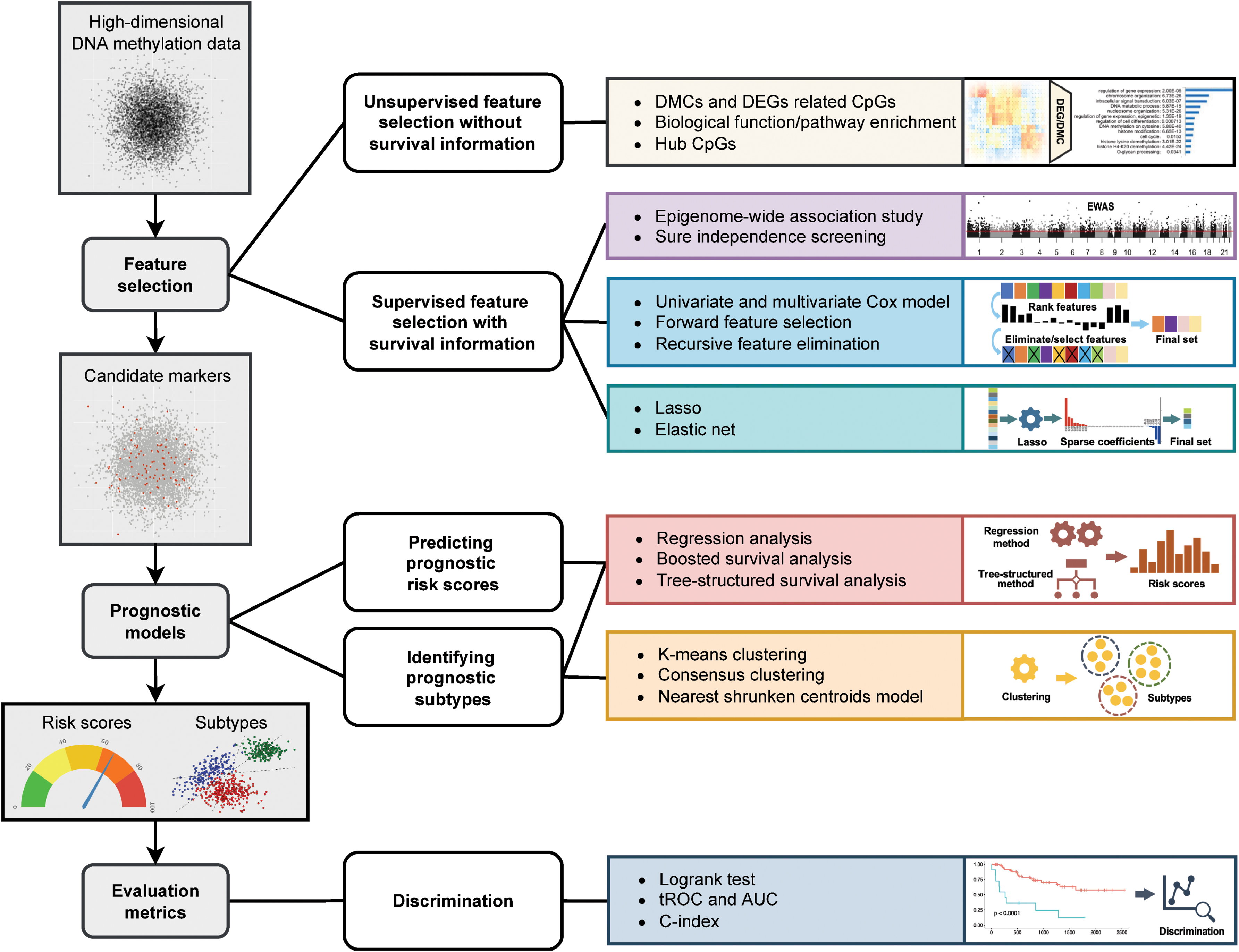
Overview of prognostic analysis of high-dimensional DNA methylation data. The left column provides the three-step procedure of prognostic analysis. First, feature selection methods identify a subset of informative markers that are associated with survival. Second, with the candidate markers, prognostic models either predict risk scores or stratify patients into subtypes. Finally, evaluation metrics are used to evaluate a model's discriminatory power. In each step, the computational methods are visualized and categorized in the right two columns. AUC, area under the ROC curve; C-index, concordance index; DEGs, differentially expressed genes; DMCs, differentially methylated CpG sites; EWAS, epigenome-wide association study; LASSO, least absolute shrinkage and selection operator; tROC, time-dependent receiver operating characteristic.

Table 1.

Summary of Reviewed Studies

Publication	Cancer type	Methylation data type	Sample size	Feature selection method	Candidate marker	Prognostic model
Predicting prognostic risk scores using tissue-based methylation
Guo et al. (2021)	Bladder cancer	Illumina 450K array	18 paired tumor and adjacent normal tissue samples for feature selection; 357 tumor samples for prognosis analysis	Differentially expressed CpG sites, Cox regression, LASSO, SVM-RFE	8 CpGs	Cox regression, nomogram
Zhang et al. (2020)	Breast cancer	Illumina 450K array	776 tumor samples	Univariate and multivariate Cox regression	6 CpGs	Cox regression
Ren et al. (2018)	Breast cancer	Illumina 450K and 27K array	8000 normal samples for feature selection; 1076 tumor samples and 122 adjacent normal tissue samples for prognosis analysis	Penalized regression	353 CpGs	Elastic net regression, Cox regression
Hao et al. (2017)	Breast cancer, lung cancer	Illumina 450K array	520 tumor samples, 65 adjacent normal tissue samples from breast cancer patients; 585 tumor samples, 49 adjacent normal tissue samples from lung cancer patients	Univariable Cox regression, LASSO, boosting	29 CpGs from LASSO and 11 CpGs from boosting for breast cancer; 75 CpGs from LASSO and 52 CpGs from boosting for lung cancer	Cox regression
Li et al. (2021)	Colorectal cancer	Illumina 450K array	307 tumor samples, 38 adjacent normal tissue samples	DMCs located near TSS and have significantly negative correlations with DEGs, SIS, and stepwise regression	10 CpGs	Cox regression
Guo et al. (2019)	Cutaneous melanoma	Illumina 450K array	461 tumor samples	Univariate and multivariate Cox regression	4 CpGs	Cox regression
Dai et al. (2021)	Gastric cancer	Illumina 450K array	395 tumor samples	CpG sites significantly associated with OS, DSS, PFI, and DFI, univariate Cox regression	7 CpGs	Cox regression
Peng et al. (2020)	Gastric cancer	Illumina 450K array	363 tumor samples	CpG sites have significantly negative correlations with DEGs, univariate and multivariate Cox regression	10 CpGs	Cox regression
Hu and Zhou (2017)	Ovarian cancer, breast cancer, and glioblastoma multiforme	Illumina 450K array	605 ovarian tumor samples, 343 breast tumor samples, and 295 glioblastoma multiforme samples	Top 10% CpG sites with the largest degrees in the DNA methylation interaction network, univariable Cox regression	76 CpGs for ovarian cancer, 69 CpGs for breast cancer, 88 CpGs for glioblastoma multiforme	Cox regression
Identifying prognostic subtypes using tissue-based methylation
Jiang et al. (2020)	ALL, AML	Illumina 450K array	194 AML samples, 136 ALL samples, and 754 normal blood samples	DMCs, univariate Cox regression	93 CpGs for ALL, 39 CpGs for AML	2-means clustering
Jiang et al. (2020)	ALL, AML	Illumina 450K array		DMCs, univariate Cox regression	23 CpGs for ALL, 20 CpGs for AML	Nearest shrunken centroids
Yang et al. (2019)	Colon adenocarcinoma	Illumina 450K and 27K array	424 tumor samples	CpGs in promoter regions, univariate and multivariate Cox regression	356 CpGs	Consensus clustering
Yang et al. (2019)	Colon adenocarcinoma	Illumina 450K and 27K array	424 tumor samples		18 CpGs	Cox regression
Feng et al. (2021)	Ovarian cancer	Illumina 450K array	108 tumor samples	DMCs, GO, and KEGG pathway enrichment analysis	8 CpGs	Binary logistic regression
Yin, Zhang et al. (2021)	Ovarian cancer	Illumina 27K array	571 tumor samples	Univariate and multivariate Cox regression	250 CpGs	Consensus clustering
Yin, Kong et al. (2021)	Pancreatic cancer	Illumina 450K array	178 tumor samples	Univariate and multivariate Cox regression	4227 CpGs	Consensus clustering
Prognostic analysis using plasma-based methylation
Zuccato et al. (2021)	Chordoma	Illumina EPIC array	68 tumor samples	Most variably methylated CpG sites	15,000 CpGs	Consensus clustering, Cox regression
Zuccato et al. (2021)	Chordoma	cfMeDIP-seq	12 matched plasma samples from patients	Top DMRs between two clusters	500 DMRs	Random forest
Luo et al. (2020)	Colorectal cancer	Targeted bisulfite sequencing	801 plasma samples from patients	Univariable Cox regression, LASSO	5 CpGs	Cox regression, nomogram
Luo et al. (2020)	Colorectal cancer	Targeted bisulfite sequencing	801 plasma samples from patients	Univariable Cox regression, LASSO	45 CpGs	Iterative consensus clustering
Xu et al. (2017)	Hepatocellular carcinoma	Targeted bisulfite sequencing	1049 plasma samples from patients	Univariable Cox regression, LASSO	8 CpGs	Cox regression

ALL, acute lymphocytic leukemia; AML, acute myelogenous leukemia; cfMeDIP-seq, cell-free methylated DNA immunoprecipitation-sequencing; DEGs, differentially expressed genes; DFI, disease-free interval; DMCs, differentially methylated CpG sites; DSS, disease-specific survival; GO, Gene Ontology; KEGG, Kyoto Encyclopedia of Genes and Genomes; LASSO, least absolute shrinkage and selection operator; OS, overall survival; PFI, progression-free interval; RFE, recursive feature elimination; SIS, sure independence screening; SVM-RFE, support vector machine recursive feature elimination; TSS, transcription start site.

To address the aforementioned challenges in analyzing high-dimensional DNA methylation data, usually a small methylation marker set is carefully screened, so survival analysis can be performed in a low-dimensional space. In this review, Section 2 presents various feature selection techniques that are applied before establishing prognostic models. Section 3 describes models used to predict the risk of death or stratify cancer prognostic subtypes. Section 4 explains different performance metrics that are used to evaluate a model's discriminatory ability. Section 5 discusses the limitations of current methods and future directions. Section 6 concludes the article.

2. METHYLATION FEATURE SELECTION

The Illumina HumanMethylation27 (27K) array and HumanMethylation450 (450K) array have been commonly used to assess the methylation status of thousands of CpGs (5′-C-phosphate-G-3′ sequence of nucleotides) across the whole genome. Recently, Illumina released the HumanMethylationEPIC (EPIC) array, which covers >850,000 CpGs distributed genome-wide (Pidsley et al., 2016). In addition to methylation arrays, high-throughput sequencing techniques, including reduced representation bisulfite sequencing (RRBS) with 2,599,828 CpG sites covered and whole genome bisulfite sequencing (WGBS) with 9,719,824 CpG sites covered (Doherty and Couldrey, 2014), can target a wider range of methylomes. These data contain a far larger number of methylation features (p) than the sample size (n).

In the high-dimensional setting (p ≫ n), classical statistical methods cannot be applied directly to predict survival (Witten and Tibshirani, 2010). Therefore, many methods have been applied to identify a subset of informative methylation features. It is also of clinical interest to identify a small number of methylation features that are highly associated with the survival outcome to simplify the prognostic model. Generally, the feature selection methods that identify DNA methylation signatures for cancer prognosis prediction can be categorized into two groups in terms of the use of survival information: (1) the methods that do not need survival information, referred to as “unsupervised” feature selection; and (2) the methods that require survival information, referred to as “supervised” feature selection.

2.1. Unsupervised feature selection without using survival information

Methylation feature selection without survival information generally starts with identifying differentially methylated CpG sites (DMCs) or differentially expressed genes (DEGs) between patients with two conditions, for example, cancer versus normal. The purpose of finding DEGs is to select methylation CpG sites located within or closely adjacent to DEGs, which are regarded to be functional. Numerous methods have been developed to identify DMCs and DEGs.

To infer DMCs from methylation array data, such as Illumina's 27K/450K/EPIC Infinium arrays, typical statistical methods include the Wilcoxon rank-sum test [offered by the IMA R package (Wang et al., 2012)] and Fisher's exact test [offered by the COHCAP R package (Warden et al., 2013)]. In addition, t-tests, analysis of variances (ANOVAs), and moderated t/F-statistics are also recommended methods (Wei et al., 2006; Chaudhary et al., 2018; Shafi et al., 2018). For differential expression analysis of gene expression data, the limma (Ritchie et al., 2015), DESeq2 (Love et al., 2014), and edgeR (Robinson et al., 2010) R packages are widely used.

Suitable approaches for identifying DMCs and DEGs can be chosen based on the objectives. For example, Feng et al. (2021) used limma to identify significant DMCs between chemoresistant and chemosensitive ovarian cancer patients. To identify methylation patterns that are correlated with DEGs, Guo et al. (2021) screened differentially expressed CpG sites between bladder tumor and adjacent normal tissues using limma. Li et al. (2021) identified DMCs by comparing all tumor and normal samples through unpaired t-tests, and paired tumor and normal samples through paired t-tests. They also identified DEGs between all tumor and normal samples as well as paired tumor and normal samples using DESeq2. Then, they filtered those DMCs located in DEGs and significant negative correlated with gene expression (Li et al., 2021). Similarly, Peng et al. (2020) acquired DEGs using edgeR and selected DNA methylation signatures of the screened DEGs whose average methylation level was significantly negatively correlated with gene expression.

In addition to DMCs, the hubs in the DNA methylation interaction network can also be candidates for cancer prognosis (Hu and Zhou, 2017). Hu and Zhou (2017) first constructed a DNA methylation interaction network by the rank correlations of DNA methylation levels in cancer samples and then chose the top 10% nodes with the largest degrees as hub methylation sites.

Identified DMCs can be further filtered with curated biological knowledge, such as the Gene Ontology (GO) (Ashburner et al., 2000) and Kyoto Encyclopedia of Genes and Genomes (KEGG) (Kanehisa and Goto, 2000) databases. DMCs or DEGs that were not significantly enriched in prognosis-relevant biological functions/pathways are filtered out. For example, Feng et al. (2021) enriched the differentially methylated genes using the GO and KEGG databases and selected candidate CpGs by their biological function.

2.2. Supervised feature selection using survival information

Supervised feature selection methods use survival information to guide the selection of features that achieve the best performance of survival prediction. There are three categories of supervised methods: filter methods, wrapper methods, and embedded methods (Guyon and Elisseeff, 2003). The procedures of wrapper and embedded methods are based on predictive models, whereas filtering methods are independent of any predictive models. In practice, due to different feature selection principles, these methods can be used in combination to find the optimal methylation feature subset.

2.2.1. Filter methods

Selecting DNA methylation sites that are truly associated with survival outcomes, such as overall survival (OS), disease-specific survival (DSS), progression-free interval (PFI), and disease-free interval (DFI), is the goal of most supervised feature selection methods. Filter methods evaluate the statistical significance of the correlation between individual methylation features and survival outcomes and keep the top-ranked features based on their correlation significance. Therefore, filter methods are generally used as a preprocessing step and are independent of any predictive models.

One example of using filter methods for feature selection is that Dai et al. (2021) conducted an epigenome-wide association study (EWAS) to screen DNA methylation markers associated with OS, DSS, PFI, and DFI. To choose optimal CpG sites for cancer prognosis prediction, Li et al. (2021) applied sure independence screening (SIS) (Fan and Lv, 2008), which selects predictors based on their correlations with the response. SIS reduces the high dimensionality to below the sample size and can be used in combination with refined lower dimensional methods such as least absolute shrinkage and selection operator (LASSO) (Fan and Lv, 2008).

2.2.2. Wrapper methods

Different from filtering methods, wrapper methods aim to search a subset of features that can achieve the best performance for a survival predictive model by evaluating all the possible combinations of variables against the evaluation criterion. Popular wrapper methods include univariate and multivariate Cox regression analyses, forward feature selection, and recursive feature elimination (RFE).

The univariate Cox proportional hazards regression model is a straightforward univariate feature selection method to find the methylation sites significantly associated with the survival of patients. Each feature is fitted with the model, and its relevance to the survival outcome can be measured by the p-value of the likelihood ratio test (De Bin et al., 2014; Hu and Zhou, 2017) or the Cox score (Beer et al., 2002; Witten and Tibshirani, 2010; Jiang et al., 2020). After the ranking of feature significance is obtained, the best combination of k features will be selected.

To choose the tuning parameter k, different strategies, such as fitting multivariate Cox proportional hazards regression models (De Bin et al., 2014) or permutation-based false discovery rate approaches (Beer et al., 2002; Witten and Tibshirani, 2010), can be applied. In practice, the univariate Cox model combined with the multivariate Cox model is widely used to identify the optimal subset of prognostic CpG sites (Guo et al., 2019; Yang et al., 2019; Peng et al., 2020; Zhang et al., 2020; Yin et al., 2021, 2021). Once the univariate and multivariate Cox regression models are fitted, one can easily calculate the hazard ratio (HR) and 95% confidence interval of individual covariates to see their association with the clinical endpoints (Ren et al., 2018).

However, a drawback of univariate feature selection is that it does not consider the correlations between features, so the most significant features may have strong correlations and are less optimal in predictive performance (De Bin et al., 2014). To alleviate this issue, wrapper methods such as forward feature selection and RFE heuristically search the optimal feature subset: using a specific survival predictive model, forward stepwise selection starts from an empty feature subset and includes one methylation feature in the model at a time if the inclusion of the feature can increase the performance one by one; in contrast, backward elimination starts from the full feature set and recursively excludes a feature whose elimination decreases the performance.

Li et al. (2021) used the strategy of stepwise selection to identify prognosis-associated CpGs. Guo et al. (2021) employed a backward elimination procedure, support vector machine recursive feature elimination (SVM-RFE), to select candidate CpGs. They ranked variables based on nonlinear SVM and SVM for survival analysis and improved the performance of the classical RFE algorithm (Guyon et al., 2002).

2.2.3. Embedded methods

Embedded approaches are implemented by survival predictive models that have built-in regularization functions. The regularized regression coefficients indicate the importance of features and, therefore, provide a natural method of feature selection. Unlike wrapper methods, embedded approaches can perform feature selection and model learning simultaneously. Since most studies used the Cox proportional hazards regression model (Cox, 1972) to predict survival, regularization, particularly shrinkage, was introduced to the Cox model. Popular examples of embedded methods are penalized Cox regression models, including LASSO, ridge, and elastic net regression.

LASSO (Tibshirani, 1996) penalizes the regression coefficients to shrink them toward zero, resulting in the selection of the most relevant variables. Subsequently, Tibshirani (1997) adapted the LASSO technique to the Cox proportional hazards regression model for survival analysis. Guo et al. (2021) and Hao et al. (2017) used LASSO to identify candidate methylation sites for classifying patients into high- and low-risk progression groups. Luo et al. (2020) and Xu et al. (2017) first used the univariate Cox method to rank features, among which the top-ranking circulating tumor DNA methylation sites were then selected by the LASSO-Cox method.

3. PROGNOSTIC MODELS

Prognostic models estimate the risk of a prognostic endpoint from multiple prognostic predictors for individual patients. Some prognostic models predict the absolute risk or relative risk that relates to the survival probability; others perform risk grouping to identify prognostic subtypes (Steyerberg et al., 2013). Although it is more accurate to provide a risk score for each patient, stratifying patients into risk groups or prognostic subtypes may inform treatment choices (Steyerberg et al., 2013). Another benefit of obtaining multiple prognostic groups is that a survival curve, which is a useful visualization and summary of the survival data, can be plotted for different groups. The Kaplan–Meier (KM) (Kaplan and Meier, 1958) survival curve is widely used to plot the KM survival probability, which is estimated nonparametrically from censored and uncensored survival times.

3.1. Predicting prognostic risk scores

A common way to calculate the risk score or prognostic index (PI) is $R i s k s c o r e = β_{1} x_{1} + β_{2} x_{2} \dots + β_{p} x_{p},$

where $x_{1}, x_{2}, \dots, x_{p}$ are covariates and $β_{1}, β_{2}, \dots, β_{p}$ are estimated coefficients. The Cox proportional hazards regression model is the most popular method for estimating the coefficients in a risk prediction model. Incorporating the screened prognosis-associated CpGs, a risk score model was used to calculate a weighted sum of methylation levels for each patient based on the regression coefficients of the Cox model (Hu and Zhou, 2017; Xu et al., 2017; Guo et al., 2019, 2021; Yang et al., 2019; Luo et al., 2020; Peng et al., 2020; Zhang et al., 2020; Dai et al., 2021; Li et al., 2021).

In addition to the Cox model, the risk score can be predicted in other ways. Ren et al. (2018) applied Horvath's (2013) elastic net regression model to calculate the DNA methylation age, which can be regarded as a special type of prognostic risk score.

The risk score predicted from methylation markers can also be integrated into an effective and intuitive nomogram model (Balachandran et al., 2015) with other clinicopathological information (e.g., age, sex, TNM stage, and primary tumor location) to predict survival (Luo et al., 2020; Guo et al., 2021; Yin et al., 2021).

In practice, most studies used risk scores to stratify cancer patients exhibiting significantly different survival probabilities. According to some cutoff points, patients are divided into two or more risk groups. For example, low- and high-risk groups are identified using the median-risk score. There are a number of ways to evaluate the prognostic value of the risk score, which shall be discussed in Section 4.

3.2. Identifying prognostic subtypes

Molecular subtypes based on DNA methylation have the potential to support the clinical stratification of patients and provide guidance for personalized treatment (Capper et al., 2018; Yang et al., 2019). An important topic related to prognosis is to determine prognosis-related molecular subtypes by DNA methylation.

Consensus clustering (Monti et al., 2003) is a robust approach that determines the cluster assignments based on multiple iterations of the clustering algorithm on subsamples. It has been applied to identify DNA methylation-based prognostic subtypes of multiple cancers (Yang et al., 2019; Yin et al., 2021, 2021; Zuccato et al., 2021). Luo et al. (2020) applied an iterative consensus clustering method to identify cell-free DNA (cfDNA) methylation-based subtypes of colorectal cancer. Then, they used the correlation coefficients between cluster centroids and samples to classify the validation data (Luo et al., 2020).

Once subtype labels are assigned to samples, a classification model can be built to predict prognostic subtypes. Jiang et al. (2020) performed 2-means clustering on training samples to obtain leukemia subtypes that differed significantly in survival. Based on the created subtype labels, they used the nearest shrunken centroids model (Tibshirani et al., 2002, 2003) to classify the validation samples into prognostic subtypes. Feng et al. (2021) classified patients into chemoresistant and chemosensitive groups using binary logistic regression. After identifying two chordoma subtypes from solid tumor samples, Zuccato et al. (2021) developed random forest models (Breiman, 2001) to classify patients into correct subtypes based on cfDNA methylation data.

3.3. Other prognostic models

In the past decade, a number of machine learning methods with built-in feature selection have been developed for survival analysis of high-dimensional data (Leger et al., 2017; Steele et al., 2018; Orozco-Sanchez et al., 2019; Spooner et al., 2020). Although they have not been widely used for DNA methylation-based cancer prognosis, they may have great potential and are presented as follows.

Tree-structured and boosted survival models can detect complex relationships among features and may provide more accurate predictions than traditional methods such as the Cox proportional hazards regression model when there is nonlinearity in the data (Bou-Hamad et al., 2011; Leger et al., 2017; Spooner et al., 2020). Hao et al. (2017) applied boosting (Friedman, 2001), which is an ensemble learning algorithm that performs wrapper-based feature selection (Alsahaf et al., 2022), to reduce the dimensionality of methylation data and construct a predictive prognostic model.

CoxBoost (Cox model with likelihood-based boosting) (Binder and Schumacher, 2008) is the best-performing algorithm in a study that systematically compared 10 survival analysis methods (Spooner et al., 2020). Leger et al. (2017) evaluated 11 methods for time-to-event survival data and recommended a few models based on boosting trees (BT), such as BT-Cox and BT-Weibull (Leger et al., 2017), random forest based methods, such as random survival forest (RSF) (Ishwaran et al., 2008) and random forest using maximally selected rank statistics (MSR-RF) (Wright et al., 2017), and the boosted gradient linear model (BGLM-Cox) (Leger et al., 2017). These models should be considered in future studies.

4. EVALUATION METRICS

To evaluate the performance of a model, two aspects of prediction capability need to be considered: (1) calibration: the predicted risk closely matches the true (observed) risk (Alba et al., 2017); and (2) discrimination: distinguish the relative risk of patients (Clark et al., 2003b). If risk estimates are accurate, a model is well calibrated; if a model adequately differentiates between those with a higher risk and those with a lower risk, it has a good discriminatory ability. Although discrimination alone is insufficient to assess a predictive model, when discrimination is inadequate, a model has no clinical value and does not need to be further tested with other metrics (Alba et al., 2017). Since most studies we reviewed do not report on calibration, the focus of this section is methods for evaluating discrimination.

Using the KM survival curve to visualize the estimated survival probabilities of two or more risk groups against time, we may intuitively see the difference between groups. Quantitatively, formal statistical tests are required to test whether the difference is statistically significant (Clark et al., 2003a). The logrank test (Peto et al., 1977) is the most popular method for comparing the survival probabilities among different risk score groups classified by cutoff points (Hao et al., 2017; Hu and Zhou, 2017; Xu et al., 2017; Guo et al., 2019, 2021; Jiang et al., 2020; Luo et al., 2020; Zhang et al., 2020; Dai et al., 2021; Feng et al., 2021; Li et al., 2021; Yin et al., 2021; Zuccato et al., 2021). The evaluation metric is the p-value of the test. Other tests, such as the Wilcoxon test (Guo et al., 2019), can also be used to detect a difference between groups. These statistical tests of significance do not provide the magnitude of the difference (Binder and Schumacher, 2008), whereas the HR measures the difference through comparison of the slopes of the curves.

A drawback of performing statistical tests on predefined risk groups is that it may not be biologically meaningful to simply use fixed thresholds to classify patients (Bøvelstad et al., 2007). To overcome this problem, metrics such as the receiver operating characteristic (ROC) curve and the area under the ROC curve (AUC) can evaluate the discriminant power of predicted risk scores without specifying rigid cutoffs. Commonly used metrics for evaluating the performance of binary classification predictions (e.g., chemoresistant vs. chemosensitive) are sensitivity, specificity, ROC curve, and AUC. In survival analysis, these metrics are slightly different because of the intervention of time. For a given survival threshold time t, the time-dependent ROC (tROC) curve (Heagerty et al., 2000; Simon et al., 2011) is plotted as sensitivity(t) versus 1 − specificity(t) or all risk score cutoffs used to define binary classes (Luo et al., 2020; Zhang et al., 2020; Guo et al., 2021), thus avoiding the use of rigid cutoffs.

The metrics presented earlier are built on the assumption that dichotomous risk groups exist. Such tests assess whether the patients are classified into the right group but overlook patients’ risk ranking within the group (Bøvelstad et al., 2007). In addition, it is more meaningful for risk to be a continuous indicator instead of a categorical label. The concordance index (c-index) (Harrell, 2001) addresses the aforementioned problems by taking the order of the risk score into account. The c-index is the probability of all pairs of patients whose predicted survival times are correctly ordered (Luo et al., 2020; Peng et al., 2020). It ranges from 0.5 (for random predictions) to 1 (for perfect predictions).

In addition to these evaluation metrics, the strategy of cross-validation (internal validation) is widely used for assessing prognostic models. Simon et al. (2011) suggested a method to derive cross-validated KM curves and tROC curves. However, the issue of data overfitting may still exist after internal validation and may prevent a prognostic model from predicting a new observation well, even though the most important features are selected and data dimensionality is significantly reduced. To address this issue, external validation using an independent data set from a different clinical setting other than the training data is an effective way to evaluate the prognostic model. In addition, external validation is a necessary step to claim whether a prognostic model is clinically useful (Steyerberg et al., 2013).

5. LIMITATIONS AND PROSPECTS

There is great potential for the discovery of methylation markers related to cancer prognosis. To date, 450K methylation arrays have dominated studies investigating the cancer methylome (Stirzaker et al., 2014), including DNA methylation-based cancer prognosis (Table 1). Although 450K detects >450,000 CpG sites that cover 96% of the CGIs (Bibikova et al., 2011), it lacks coverage of genomic regions such as distal regulatory elements (Pidsley et al., 2016). The methylation changes beyond CGIs, CGI shores, and shelves are largely overlooked (Strand et al., 2014). With the development of sequencing technology, we believe there will be growth in the identification of novel prognostic markers beyond the currently investigated genomic regions.

Choosing proper feature selection methods and their suitable hyperparameters is critical yet challenging for analyzing high-dimensional DNA methylation data. Although different approaches or combinations of multiple approaches have been used for different data sets in the literature, there is a need for a systematic investigation and comparison of various feature selection methods. In addition, the number of features required to achieve optimal performance is debatable. The traditional Cox model is the most commonly used model for multivariate biomarker discovery and survival analysis; however, it can only use a small number of significant markers because the maximum number of variables it allows depends on the incidence rate (or hazard) (van Dijk et al., 2008). As more machine learning algorithms designed for high-dimensional survival data are being invented, we envision that increased sensitivity and specificity for cancer prognosis can be achieved with larger marker panels.

Feature selection is expected to reduce overfitting and improve accuracy. However, it is not always the case that it can optimize the performance of a prognostic model. Machine learning approaches, including random forest methods and boosted survival models, provide efficient and highly competitive solutions to the issue of high dimensionality. Such prognostic models are adapted to a variety of wrapper or embedded methods to deal with high-dimensional data, so extra regularization and subset selection steps may not need to be taken (Pölsterl et al., 2016; Orozco-Sanchez et al., 2019; Spooner et al., 2020).

In addition to features selection methods, dimensionality reduction techniques can be considered. Unlike feature selection that selects or excludes features without transformation, dimensionality reduction maps high-dimensional data into a latent space with lower dimensionality. For example, deep learning-based methods such as autoencoders have been applied to reduce the dimensionality of multiomics data, including DNA methylation, and showed improved performance in survival prediction (Chaudhary et al., 2018; Zhang et al., 2021).

The accurate prediction of prognostic outcomes generally requires multiple prognostic predictors (Steyerberg et al., 2013). Although omics research investigates a wide range of biological factors (including genomic, epigenomic, transcriptomic, proteomic, and metabolomic features) for cancer prognosis, classical clinical predictors alone can often provide reasonably satisfying results. It is, therefore, reasonable to combine methylation signatures with clinicopathological information to improve the prognostic estimation (Luo et al., 2020). Adding clinical factors to the model can also adjust for potential confounders such as patient age (Dai et al., 2021; Zuccato et al., 2021).

If the association between prognostic factors and clinical outcomes is weak, it may not always be the problem of feature selection methods or prognostic models. Noisy survival outcomes can be the cause of unsatisfactory performance. Many studies focus on predicting OS, which includes all people surviving all causes of death. As time elapsed, more patients died of diseases other than cancer, thus increasing the noise in the OS endpoint. Recurrence-free survival may be a better outcome for estimating cancer-specific prognosis (Ren et al., 2018). Furthermore, benchmark databases labeled by experts are urgently needed for validating and comparing prognosis methods (Zhu et al., 2020).

6. CONCLUSION

Compared with other genomic data (e.g., gene expression), high-dimensional DNA methylation data for cancer prognosis have not been extensively studied. Most studies have mainly focused on using DNA methylation data to identify cancer subtypes (molecular typing of cancer), identify markers for cancer diagnosis, or stratify patients for treatment. Prognosis analysis is usually a minor or add-on part of the study. In those studies, DNA methylation markers associated with survival were usually identified using various feature selection methods.

A traditional Cox model is commonly used to characterize the relationship between methylation features and survival outcomes. For model evaluation, we suggest using multiple metrics for a comprehensive assessment since different metrics assess different perspectives of the discriminatory ability of survival prediction models. Given that DNA methylation dynamically and precisely captures the pathological states of organs, we believe that there is great potential for the development of more machine learning algorithms to harness high-dimensional methylation data in analyzing censored cancer survival data.

Footnotes

AUTHORS’ CONTRIBUTIONS

R.H. performed literature survey and article preparation. W.L. and X.J.Z provided conceptualization, editing, and supervision.

AUTHOR DISCLOSURE STATEMENT

X.J.Z. and W.L. are cofounders of EarlyDiagnostics, Inc. The other authors declare no competing interests.

FUNDING INFORMATION

This research is supported by the National Cancer Institute (Grant Nos. U01CA230705 to X.J.Z., R01CA246329 to X.J.Z. and W.L., and U01CA237711 to W.L.).

References

Alba

A.C.

, Agoritsas

, Walsh

, et al. 2017. Discrimination and calibration of clinical prediction models: users’ guides to the medical literature. JAMA, 318, 1377–1384.

Alsahaf

, Petkov

, Shenoy

, et al. 2022. A framework for feature selection through boosting. Expert Syst. Appl. 187, 115895.

Ashburner

, Ball

C.A.

, Blake

J.A.

, et al. 2000. Gene ontology: tool for the unification of biology. Nat. Genet. 25, 25–29.

Balachandran

V.P.

, Gonen

, Smith

J.J.

, et al. 2015. Nomograms in oncology: more than meets the eye. Lancet Oncol. 16, e173–e180.

Beer

D.G.

, Kardia

S.L.

, Huang

C.-C.

, et al. 2002. Gene-expression profiles predict survival of patients with lung adenocarcinoma. Nat. Med. 8, 816–824.

Bibikova

, Barnes

, Tsan

, et al. 2011. High density DNA methylation array with single CpG site resolution. Genomics, 98, 288–295.

Binder

, and Schumacher

2008. Allowing for mandatory covariates in boosting estimation of sparse high-dimensional survival models. BMC Bioinform. 9, 1–10.

Bou-Hamad

, Larocque

, and Ben-Ameur

2011. A review of survival trees. Stat. Surv. 5, 44–71.

Boulesteix

A.-L.

, and Sauerbrei

2011. Added predictive value of high-throughput molecular data to clinical data and its validation. Brief. Bioinform. 12, 215–229.

10.

Bøvelstad

H.M.

, Nygård

, Størvold

H.L.

, et al. 2007. Predicting survival from microarray data—a comparative study. Bioinformatics, 23, 2080–2087.

11.

Breiman

2001. Random forests. Mach. Learn. 45, 5–32.

12.

Capper

, Jones

D.T.

, Sill

, et al. 2018. DNA methylation-based classification of central nervous system tumours. Nature, 555, 469–474.

13.

Chaudhary

, Poirion

O.B.

, Lu

, et al. 2018. Deep learning-based multi-omics integration robustly predicts survival in liver cancer. Clin. Cancer Res. 24, 1248–1259.

14.

Clark

T.G.

, Bradburn

M.J.

, Love

S.B.

, et al. 2003a. Survival analysis part I: basic concepts and first analyses. Br. J. Cancer 89, 232–238.

15.

Clark

T.G.

, Bradburn

M.J.

, Love

S.B.

, et al. 2003b. Survival analysis part IV: further concepts and methods in survival analysis. Br. J. Cancer 89, 781–786.

16.

Cox

D.R.

1972. Regression models and life-tables. J. R. Stat. Soc. Ser. B Methodol. 34, 187–202.

17.

Dai

, Nishi

, Li

Z.-X.

, et al. 2021. DNA methylation signatures associated with prognosis of gastric cancer. BMC Cancer, 21, 1–14.

18.

De Bin

, Sauerbrei

, and Boulesteix

A.L.

2014. Investigating the prediction ability of survival models based on both clinical and omics data: two case studies. Stat. Med. 33, 5310–5329.

19.

Doherty

, and Couldrey

2014. Exploring genome wide bisulfite sequencing for DNA methylation analysis in livestock: a technical assessment. Front. Genet. 5, 126.

20.

Fan

, and Lv

2008. Sure independence screening for ultrahigh dimensional feature space. J. R. Stat. Soc. Ser. B Methodol. 70, 849–911.

21.

Feng

.-y., Yan

.-b., Huang

.-z., et al. 2021. Abnormal methylation characteristics predict chemoresistance and poor prognosis in advanced high-grade serous ovarian cancer. Clin. Epigenetics, 13, 1–18.

22.

Friedman

J.H.

2001. Greedy function approximation: a gradient boosting machine. Ann. Stat. 1189–1232.

23.

Guo

, Zhu

, et al. 2019. A four-DNA methylation biomarker is a superior predictor of survival of patients with cutaneous melanoma. Elife, 8, e44310.

24.

Guo

, Yin

, Dai

, et al. 2021. A novel CpG methylation risk indicator for predicting prognosis in bladder cancer. Front. Cell Dev. Biol. 9, 642650.

25.

Guyon

, and Elisseeff

2003. An introduction to variable and feature selection. J. Mach. Learn. Res. 3, 1157–1182.

26.

Guyon

, Weston

, Barnhill

, et al. 2002. Gene selection for cancer classification using support vector machines. Mach. Learn. 46, 389–422.

27.

Hao

, Luo

, Krawczyk

, et al. 2017. DNA methylation markers for diagnosis and prognosis of common cancers. Proc. Natl. Acad. Sci. U.S.A. 114, 7414–7419.

28.

Harrell

F.E.

2001. Regression Modeling Strategies: With Applications to Linear Models, Logistic Regression, and Survival Analysis. Springer, New York.

29.

Heagerty

P.J.

, Lumley

, and Pepe

M.S.

2000. Time-dependent ROC curves for censored survival data and a diagnostic marker. Biometrics, 56, 337–344.

30.

Heyn

, and Esteller

2012. DNA methylation profiling in the clinic: applications and challenges. Nat. Rev. Genet. 13, 679–692.

31.

Horvath

2013. DNA methylation age of human tissues and cell types. Genome Biol. 14, 1–20.

32.

W.-L.

, and Zhou

X.-H.

2017. Identification of prognostic signature in cancer based on DNA methylation interaction network. BMC Med. Genomics, 10, 81–91.

33.

Ishwaran

, Kogalur

U.B.

, Blackstone

E.H.

, et al. 2008. Random survival forests. Ann. Appl. Stat. 2, 841–860.

34.

Jiang

, Ou

, He

, et al. 2020. DNA methylation markers in the diagnosis and prognosis of common leukemias. Signal Transduct. Target. Ther. 5, 1–10.

35.

Kanehisa

, and Goto

2000. KEGG: kyoto encyclopedia of genes and genomes. Nucleic Acids Res. 28, 27–30.

36.

Kaplan

E.L.

, and Meier

1958. Nonparametric estimation from incomplete observations. J. Am. Stat. Assoc. 53, 457–481.

37.

Leger

, Zwanenburg

, Pilz

, et al. 2017. A comparative study of machine learning methods for time-to-event survival data for radiomics risk modelling. Sci. Rep. 7, 1–11.

38.

Leung

K.-M.

, Elashoff

R.M.

, and Afifi

A.A.

1997. Censoring issues in survival analysis. Annu. Rev. Public Health, 18, 83–104.

39.

D.-H.

, Du

X.-H.

, Liu

, et al. 2021. A 10-gene-methylation-based signature for prognosis prediction of colorectal cancer. Cancer Genet. 252, 80–86.

40.

Love

M.I.

, Huber

, and Anders

2014. Moderated estimation of fold change and dispersion for RNA-seq data with DESeq2. Genome Biol. 15, 1–21.

41.

Luo

, Zhao

, Wei

, et al. 2020. Circulating tumor DNA methylation profiles enable early diagnosis, prognosis prediction, and screening for colorectal cancer. Sci. Transl. Med. 12, eaax7533.

42.

Mallik

, and Zhao

2020. Graph-and rule-based learning algorithms: a comprehensive review of their applications for cancer type classification and prognosis using genomic data. Brief. Bioinform. 21, 368–394.

43.

Monti

, Tamayo

, Mesirov

, et al. 2003. Consensus clustering: a resampling-based method for class discovery and visualization of gene expression microarray data. Mach. Learn. 52, 91–118.

44.

Orozco-Sanchez

, Trevino

, Martinez-Ledesma

, et al. 2019. Exploring survival models associated with MCI to AD conversion: a machine learning approach. bioRxiv 836510.

45.

Peng

, Wu

, Wang

, et al. 2020. A DNA methylation signature to improve survival prediction of gastric cancer. Clin. Epigenetics, 12, 1–16.

46.

Peto

, Pike

, Armitage

, et al. 1977. Design and analysis of randomized clinical trials requiring prolonged observation of each patient. II. analysis and examples. Br. J. Cancer, 35, 1–39.

47.

Pidsley

, Zotenko

, Peters

T.J.

, et al. 2016. Critical evaluation of the Illumina MethylationEPIC BeadChip microarray for whole-genome DNA methylation profiling. Genome Biol. 17, 1–17.

48.

Pölsterl

, Conjeti

, Navab

, et al. 2016. Survival analysis for high-dimensional, heterogeneous medical data: exploring feature extraction as an alternative to feature selection. Artif. Intell. Med. 72, 1–11.

49.

Rampatige

, Gamage

, Peiris

, et al. 2013. Assessing the reliability of causes of death reported by the Vital Registration System in Sri Lanka: medical records review in Colombo. Health Inf. Manag. J. 42, 20–28.

50.

Ren

, Du

, Li

, et al. 2019. Robust network-based regularization and variable selection for high-dimensional genomic data in cancer prognosis. Genet. Epidemiol. 43, 276–291.

51.

Ren

J.-T.

, Wang

M.-X.

, Su

, et al. 2018. Decelerated DNA methylation age predicts poor prognosis of breast cancer. BMC Cancer, 18, 1–8.

52.

Ritchie

M.E.

, Phipson

, Wu

, et al. 2015. limma powers differential expression analyses for RNA-sequencing and microarray studies. Nucleic Acids Res. 43, e47.

53.

Robinson

M.D.

, McCarthy

D.J.

, and Smyth

G.K.

2010. edgeR: a Bioconductor package for differential expression analysis of digital gene expression data. Bioinformatics, 26, 139–140.

54.

Shafi

, Mitrea

, Nguyen

, et al. 2018. A survey of the approaches for identifying differential methylation using bisulfite sequencing data. Brief. Bioinform. 19, 737–753.

55.

Simon

R.M.

, Subramanian

, Li

M.-C.

, et al. 2011. Using cross-validation to evaluate predictive accuracy of survival risk classifiers based on high-dimensional data. Brief. Bioinform. 12, 203–214.

56.

Spooner

, Chen

, Sowmya

, et al. 2020. A comparison of machine learning methods for survival analysis of high-dimensional clinical data for dementia prediction. Sci. Rep. 10, 1–10.

57.

Steele

A.J.

, Denaxas

S.C.

, Shah

A.D.

, et al. 2018. Machine learning models in electronic health records can outperform conventional survival models for predicting patient mortality in coronary artery disease. PLoS One, 13, e0202344.

58.

Steyerberg

E.W.

, Moons

K.G.

, van der Windt

D.A.

, et al. 2013. Prognosis Research Strategy (PROGRESS) 3: prognostic model research. PLoS Med. 10, e1001381.

59.

Stirzaker

, Taberlay

P.C.

, Statham

A.L.

, et al. 2014. Mining cancer methylomes: prospects and challenges. Trends Genet. 30, 75–84.

60.

Strand

S.H.

, Orntoft

T.F.

, and Sorensen

K.D.

2014. Prognostic DNA methylation markers for prostate cancer. Int. J. Mol. Sci. 15, 16544–16576.

61.

Tibshirani

1996. Regression shrinkage and selection via the Lasso. J. R. Stat. Soc. Ser. B Methodol. 58, 267–288.

62.

Tibshirani

1997. The lasso method for variable selection in the Cox model. Stat. Med. 16, 385–395.

63.

Tibshirani

, Hastie

, Narasimhan

, et al. 2002. Diagnosis of multiple cancer types by shrunken centroids of gene expression. Proc. Natl. Acad. Sci. U.S.A. 99, 6567–6572.

64.

Tibshirani

, Hastie

, Narasimhan

, et al. 2003. Class prediction by nearest shrunken centroids, with applications to DNA microarrays. Stat. Sci. 18, 104–117.

65.

Van Dijk

P.C.

, Jager

K.J.

, Zwinderman

A.H.

, et al. 2008. The analysis of survival data in nephrology: basic concepts and methods of Cox regression. Kidney Int. 74, 705–709.

66.

Van Wieringen

W.N.

, Kun

, Hampel

, et al. 2009. Survival prediction using gene expression data: a review and comparison. Comput. Stat. Data Anal. 53, 1590–1603.

67.

Wang

, Yan

, Hu

, et al. 2012. IMA: an R package for high-throughput analysis of Illumina's 450K Infinium methylation data. Bioinformatics, 28, 729–730.

68.

Warden

C.D.

, Lee

, Tompkins

J.D.

, et al. 2013. COHCAP: an integrative genomic pipeline for single-nucleotide resolution DNA methylation analysis. Nucleic Acids Res. 41, e117–e117.

69.

Wei

S.H.

, Balch

, Paik

H.H.

, et al. 2006. Prognostic DNA methylation biomarkers in ovarian cancer. Clin. Cancer Res. 12, 2788–2794.

70.

Witten

D.M.

, and Tibshirani

2010. Survival analysis with high-dimensional covariates. Stat. Methods Med. Res. 19, 29–51.

71.

Wright

M.N.

, Dankowski

, Ziegler

2017. Unbiased split variable selection for random survival forests using maximally selected rank statistics. Stat. Med. 36, 1272–1284.

72.

, Fengji

, Changning

, et al. 2015. Comparison of the prognostic utility of the diverse molecular data among lncRNA, DNA Methylation, microRNA, and mRNA across five human cancers. PLoS One, 10, e0142433.

73.

.-h., Wei

, Krawczyk

, et al. 2017. Circulating tumour DNA methylation markers for diagnosis and prognosis of hepatocellular carcinoma. Nat. Mater. 16, 1155–1161.

74.

Yang

, Zhang

, Xu

, et al. 2019. Molecular subtypes based on DNA methylation predict prognosis in colon adenocarcinoma patients. Aging (Albany NY), 11, 11880.

75.

Yin

, Zhang

, Yang

2021. DNA methylation subtypes for ovarian cancer prognosis. FEBS Open Bio, 11, 851–865.

76.

Yin

, Kong

, and Liu

2021. Identification of prognosis-related molecular subgroups based on DNA methylation in pancreatic cancer. Clin. Epigenetics, 13, 1–16.

77.

Zhang

, Wang

, et al. 2020. Integrative analysis of DNA methylation and gene expression to determine specific diagnostic biomarkers and prognostic biomarkers of breast cancer. Front. Cell Dev. Biol. 8, 1535.

78.

Zhang

, Xing

, Sun

, et al. 2021. OmiEmbed: a unified multi-task deep learning framework for multi-omics data. Cancers, 13, 3047.

79.

Zhu

, Xie

, Han

, et al. 2020. The application of deep learning in cancer prognosis prediction. Cancers, 12, 603.

80.

Zuccato

J.A.

, Patil

, Mansouri

, et al. 2021. DNA Methylation based prognostic subtypes of chordoma tumors in tissue and plasma. Neuro Oncol. 24, 442–454.

Computational Analysis of High-Dimensional DNA Methylation Data for Cancer Prognosis

Abstract

1. INTRODUCTION

2.1. Unsupervised feature selection without using survival information

2.2. Supervised feature selection using survival information

2.2.1. Filter methods

2.2.2. Wrapper methods

2.2.3. Embedded methods

3. PROGNOSTIC MODELS

3.1. Predicting prognostic risk scores

3.2. Identifying prognostic subtypes

3.3. Other prognostic models

4. EVALUATION METRICS

5. LIMITATIONS AND PROSPECTS

6. CONCLUSION

Footnotes

AUTHORS’ CONTRIBUTIONS

AUTHOR DISCLOSURE STATEMENT

FUNDING INFORMATION

References