Sage Journals: Discover world-class research

Abstract

Microbial organisms play important roles in many aspects of human health and diseases. Encouraged by the numerous studies that show the association between microbiomes and human diseases, computational and machine learning methods have been recently developed to generate and utilize microbiome features for prediction of host phenotypes such as disease versus healthy cancer immunotherapy responder versus nonresponder. We have previously developed a subtractive assembly approach, which focuses on extraction and assembly of differential reads from metagenomic data sets that are likely sampled from differential genomes or genes between two groups of microbiome data sets (e.g., healthy vs. disease). In this article, we further improved our subtractive assembly approach by utilizing groups of k-mers with similar abundance profiles across multiple samples. We implemented a locality-sensitive hashing (LSH)-enabled approach (called kmerLSHSA) to group billions of k-mers into k-mer coabundance groups (kCAGs), which were subsequently used for the retrieval of differential kCAGs for subtractive assembly. Testing of the kmerLSHSA approach on simulated data sets and real microbiome data sets showed that, compared with the conventional approach that utilizes all genes, our approach can quickly identify differential genes that can be used for building promising predictive models for microbiome-based host phenotype prediction. We also discussed other potential applications of LSH-enabled clustering of k-mers according to their abundance profiles across multiple microbiome samples.

1. Introduction

Recent studies of microbiomes (i.e., communities of microorganisms) have shaped a new view of the biological world in which various microbial organisms play important roles in the health of humans, animals, plants, and the environment (Altamirano-Barrera et al., 2018; Dai et al., 2018; Haase et al., 2018; Zhao et al., 2018). Perturbations of the gut microbiota structure are associated with intestinal diseases including cancer.

Metagenome-wide association studies (Wang and Jia, 2016) have enabled the high-resolution discovery of associations between the microbiome and various human diseases, including type 2 diabetes (T2D) (Qin et al., 2012), liver cirrhosis (LC) (Qin et al., 2014), atherosclerotic cardiovascular disease (Jie et al., 2017), colorectal cancer (Zeller et al., 2014; Silva et al., 2021), and rheumatoid arthritis (Zhang et al., 2015). A recent comprehensive analysis of the tumor microbiome involving >1000 tumors and their adjacent normal tissues across seven cancer types revealed that each tumor type has a distinct microbiome composition and that breast cancer has a particularly rich and diverse microbiome (Nejman et al., 2020).

Using microbial markers that are differential between healthy individuals and patients, predictive models with promising accuracy have been built for predicting host phenotypes based on microbiome data (Qin et al., 2014; Le Goallec et al., 2020). In such studies, various microbial features are extracted from metagenome samples, including the marker genes/species or compositional changes between the samples of distinct phenotypes. For instance, in an earlier LC study, a set of mere 15 microbial marker genes was used to build a predictor that had an area under the ROC curve (AUC) of 0.91 for discrimination of patients from healthy individuals (Qin et al., 2014).

In another research, the metagenome-wide association study of fecal, dental, and salivary samples was performed on a cohort of individuals with rheumatoid arthritis (RA) (Zhang et al., 2015); dysbiosis was detected in the gut and oral microbiomes of RA patients and Haemophilus spp. was depleted and negatively correlated with levels of serum autoantibodies, whereas Lactobacillus salivarius was over-represented in individuals with RA at all three sites.

A multiomic approach that integrated metagenomics, metatranscriptomics, and proteomics was adopted to characterize the microbiome associated with different parts of the intestines of the patients with the inflammatory bowel diseases (IBDs); it was found that the gut microbiome stability (measured by the metagenomic, metatranscriptomic, and metabolomic profiles) in IBD patients decreased more from the baseline over time (Lloyd-Price et al., 2019).

Microbiome-based human host phenotype prediction has benefited from the recent advance of machine learning (ML) algorithms. A recent effort mined microbial reads in the whole genome and transcriptome sequencing data from different cancer types acquired by The Cancer Genome Atlas (TCGA) project, and revealed unique microbial signatures in tissues and blood within and between most major cancer types, resulting in microbiome-based predictive models that can distinguish different cancer types and stages (Poore et al., 2020). Statistical Inference of Associations between Microbial Communities And host phenoTypes (SIAMCAT) is a ML toolbox developed to address the issues related to ML algorithms in microbiome studies such as the poor generalization (Wirbel et al., 2021).

By comparing the prediction performances and the biological interpretation across multiple ML methods and different types of metagenomic data, Le Goallec et al. (2020) showed that the prediction accuracy depended on the choice of ML algorithms and features, and presented a computational framework for inferring microbiome-derived features of host phenotypes. Deep learning methods including various autoencoders were also exploited for learning the representation of quantitative microbiome profile in a lower dimensional latent space, which were used for building predictive models for host disease prediction (Oh and Zhang, 2020).

We previously developed a novel computational approach (CoSA: Concurrent Subtractive Assembly) (Han et al., 2017) for extracting differential bacterial genes by first detecting differential k-mers and then differential reads, followed by the downstream assembly of the differential reads. The annotation of the subtractive assembly leads to the rapid identification of differential genes that can be used as features for microbiome-based phenotype prediction. We further applied CoSA to several microbiome data sets of human diseases, which were collected and disseminated for testing new methods for deriving microbial features and for developing predictive models by a broad research community (Han and Ye, 2018).

The CoSA approach worked well on simulated data sets and some real microbiome data sets; however, its performance was still limited for some microbiome data sets, particularly for those with complex community structure (e.g., the gut microbiome data sets from the patients with nonsmall-cell lung cancer [NSCLC] that responded to cancer immunotherapy; see Section 3). To overcome this limitation, we proposed to exploit the clusters of k-mers sharing similar abundance profiles across multiple samples to improve the detection of differential k-mers between samples of different host phenotypes and thus to improve the characterization of differential reads and genes for downstream analyses.

It was shown that gene-centric predictive models, which use genes or coabundance groups of genes (CAGs), achieved superior performance compared with composition-based predictive models for microbiome-based host phenotype prediction (Le Goallec et al., 2020). Gene-centric approaches typically involve a few steps that are computationally intensive, including the assembly of the metagenomic sequences, the prediction of genes from the assemblies, the generation of nonredundant gene collection, followed by the quantification of genes (by reads mapping) and the selection of differential abundant genes that can be used as features.

The conventional approaches typically result in gigantic collections of microbial genes (Qin et al., 2010; Kim et al., 2021), imposing challenges for selecting features to be used in the predictive models. Our CoSA approach dramatically reduces the size of the putative genes to be selected as features. We show here that our new approach that utilizes clusters of differential k-mers further enhances the ability of the subtractive assembly approach, generating only a small collection of genes that can be used in the downstream analyses for assembling differential genes and building predictive models.

2. Methods

2.1. Overview of kmerLSHSA

We developed kmerLSHSA for subtractive assembly and characterization of genes from microbiome data that are associated with the host phenotype. It is an extension of our previously developed subtractive assembly approach CoSA (Han et al., 2017). The kmerLSHSA method relies on the detection of the differential k-mer coabundance groups (kCAGs), which will be subsequently used for the extraction of differential reads between two groups of microbiome data sets (e.g., healthy vs. diseased).

In this study, a kCAG represents a group of k-mers that share similar abundance profiles across multiple samples, and thus are likely from the same or co-occurring microbial genomes/genes. Figure 1 shows the workflow of kmerLSHSA, including the key steps of building k-mer abundance profiles and using locality-sensitive hashing (LSH) to group k-mers into kCAGs.

FIG. 1.

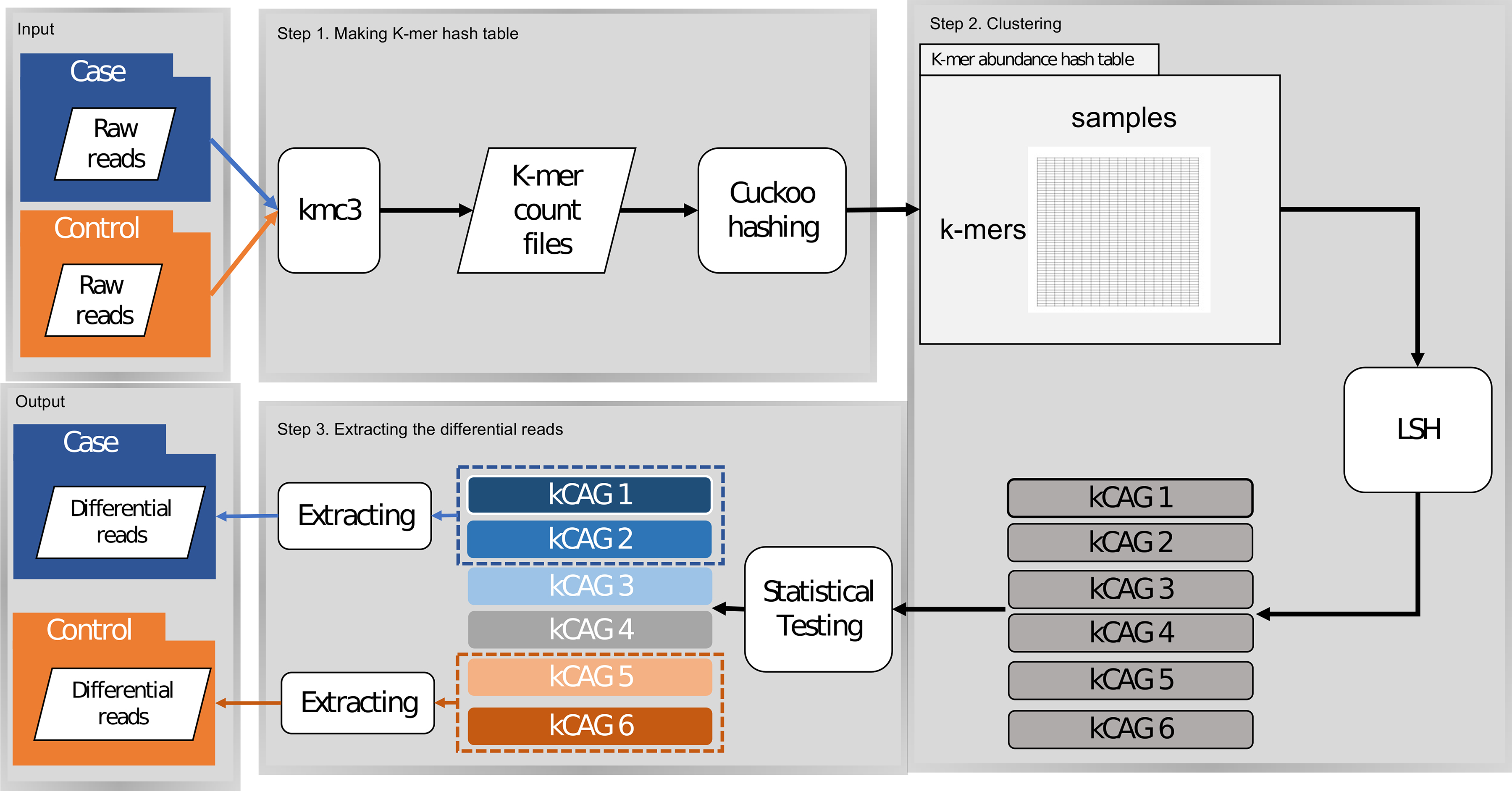
The schematic illustration of the kmerLSHSA workflow. kCAGs, k-mer coabundance groups; LSH, locality-sensitive hashing.

2.2. Building k-mer abundance profiles

The first step of kmerLSHSA is to count all k-mers in metagenomic samples. For comparative metagenomic studies, the sheer size of the data sets is a fundamental challenge. KMC3 (Kokot et al., 2017) is used for k-mer counting, setting the maximal count (the –cs flag) as 65,536 instead of 255 (the default). Using a larger cutoff helps identify more frequently observed differential k-mers; in addition, each counter can be represented using a 16-bit unsigned integer, demanding a reasonable amount of memory or disk space for storing counts of billions of k-mers across multiple samples.

Meanwhile, we exclude k-mers occurring less than two times by the –ci option (minimum count) considering they are likely from sequencing errors, a practice that was previously adopted by KMC2 (Deorowicz et al., 2015), 2BFCounter (Melsted and Pritchard, 2011), and khmer (Zhang et al., 2014). We used k = 23, which was selected empirically, balancing the memory assumption and the performance of kmerLSHSA.

After the k-mer counting using KMC3, kmerLSHSA processes the output of KMC3 by using the KMC Application Programming Interface (API), and exports all observed k-mers in a hash table, implemented using the libcuckoo library (downloaded from https://github.com/efficient/libcuckoo). Libcuckoo (Li et al., 2014) provides a high-performance concurrent hash table, by which we can efficiently update the hash table using multiple threads. With the k-mers in the hash table, kmerLSHSA parses the output of KMC2 for the second time and exports the counts of the k-mers onto hard disk following their order in the hash table of every sample. By storing the counts on the disk, kmerLSHSA loads the counts of k-mers in batches and, therefore, significantly reduces the memory requirement for recording the counts of all k-mers in every sample.

To compute the abundance profile, kmerLSHSA first computes the count of each k-mer in each metagenomic sample (to account for the low count of a rare k-mer, the k-mer count is represented as the number of occurrences per million k-mers), and then normalizes the count by the centered log ratio (CLR) count.

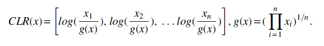
The CLR approach is capable of removing the unit-sum constraint of compositional data (Aitchison, 1982), and thus is less sensitive to the outliers than the total sum normalization approach (which was used by CoSA).

2.3. Generating kCAG by LSH

Given the massive set of k-mers in the metagenomic sequences acquired from multiple microbiome samples, we aim to cluster these k-mers into groups of k-mers with similar abundance profiles across these samples, referred to as the kCAGs. We view the k-mer clustering problem as a high dimensional vector clustering problem: each k-mer is represented by an abundance vector in which each dimension represents the normalized count of the k-mer in a sample, and the similarity between two k-mers is then measured by the cosine of the angle between their respective abundance vectors. Because the number of k-mers in a metagenomic data set is huge (in billions), we devised a fast clustering algorithm enabled by LSH to group the k-mers into kCAGs.

Notably, LSH was previously used to speed up sequence comparison. Specifically, the LSH method MinHash was used to rapidly detect highly similar sequences in genomic data sets (Ondov et al., 2016; Marçais et al., 2019), and was adopted for the detection of contaminated reads in genomic/metagenomic sequences (Ondov et al., 2019) and for the clustering of sequences from ChIP-seq data (Soto et al., 2019).

However, the goal of these methods is considerably different from the kmerLSHSA approach: although these methods attempt to cluster genomic sequences based on their sequence similarities, kmerLSHSA attempts to cluster k-mers based on their abundance profiles across multiple samples. In fact, we have previously adopted LSH for clustering tandem mass spectra (Wang et al., 2018), which is a similar computational problem as the one studied in this article.

In general, LSH is defined as follows: Let H be a family of hash functions h that maps objects in a metric space M to a bucket $s \in S$ . The family of hash functions H is called locality sensitive under a distance threshold R and the collision probability P₁ and P₂ $(P_{1} > P_{2})$ if for any two objects $p, q \in M$ : $i f d (p, q) \leq R, t h e n P r [h (p) = h (q)] \geq P_{1},$ $i f d (p, q) \geq c R, t h e n P r [h (p) = h (q)] \leq P_{2} w h e r e (c > 1),$

where $d (p, q)$ is the distance between the objects p and q, and $P r [h (p) = h (q)]$ represents the probability that p and q collide under a hash function. Specifically, in this article, we used a family of LSH functions called SimHash (Charikar, 2002; Andoni and Indyk, 2006) to approximate the cosine similarity measure between abundance vectors using random projection (Wang et al., 2014).

For a given input vector x, the SimHash function is defined as $h (x) = s i g n (w^{T} x),$ where w is a randomly chosen vector, and $h (x) = + 1$ or $- 1$ depending on which side of the hyperplane (with normal vector of w) x lies. For any two vectors s_i and s_j, $P r [h (s_{i}) = h (s_{j})] = 1 - \frac{θ (s_{i}, s_{j})}{π}$ . Hence, the higher the cosine similarity (i.e., smaller $θ$ ) between the two vectors, the more probable they are mapped to the same side of the hyperplane. Here, each side of the hyperplane is considered as a bucket, and thus a single SimHash function h defines a hash table of two buckets.

The key idea of SimHash-based k-mer clustering is to map k-mers into many buckets such that those sharing similar abundance vectors are likely to be mapped into the same buckets. To cluster the large number of k-mers, we just need to examine the similarities between the abundance vectors of the k-mers in the same bucket. Therefore, we hope to create a hash table with millions of buckets (for storing billions of k-mers) so that on average a small number of k-mers are mapped to each bucket. To create the hash table with many buckets, we construct a compound hash function $g (x) = (h_{1} (x), \dots, h_{n} (x))$ by concatenating n SimHash functions, $h_{1} (x), \dots, h_{n} (x)$ , where each function $h_{i} (x)$ is chosen randomly from the family $ℋ$ (Wang et al., 2014).

When the compound hash functions are used, the LSH algorithm amplifies the gap of the collision probability between the k-mers with similar abundance profiles and k-mers with dissimilar abundance profiles. In particular, two k-mers are mapped into the same bucket in a hash table of n concatenated SimHash functions, only if they have the same compound hash keys; hence for two k-mers with a collision probability p under a single SimHash function h, their collision probability under the compound hash function becomes pⁿ, which means two k-mers of similar abundance profiles may be mapped to different buckets (i.e., the false negatives) with a probability of $1 - p^{n}$ .

To reduce these false negatives in the LSH algorithm, we implemented an iterative approach: the k-mers are clustered in L steps, in each step, the k-mers with abundance profile similarity greater than a threshold are expected to be clustered, and the threshold gradually decreases from a preset maximum value (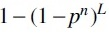 $p_{m a x}$ ) to a minimum value ( $p_{m i n}$ ) in L steps. Therefore, the overall collision probability of two k-mers with similar abundance vectors (cosine $\geq p_{m i n}$ ) becomes .

For example, when we use a compound hash function with 20 SimHash functions and 100 iterations, the collision probability is $\approx 0.98$ for the abundance profile similarity (p) of 0.85, which means $98 %$ of k-mers pairs with the abundance vectors of the similarity $0.85$ or higher will be mapped into at least one bucket after 100 iterations. In kmerLSHSA, the number of hash functions (n) is automatically determined according to the number of k-mers to be clustered (N), $⌊ l o g_{2} N ⌋$ . By default, $p_{m a x}$ and $p_{m i n}$ are set to be 0.95 and 0.85, and L is set to be 100.

One issue in the application of LSH-enabled clustering algorithm is that the k-mers are often not evenly distributed in the buckets. As a result, a few rich buckets may contain many k-mers while most buckets contain a small number of k-mers. In this case, the clustering algorithm still needs to examine the pairwise abundance profile similarities among many k-mers in the rich bucket, making the algorithm slower. To address this issue, we adopted a nested LSH approach that includes an outerLSH as a typical compound LSH as already described, and an innerLSH, a compound LSH with fewer (default 15) concatenated SimHash functions, that is only applied to the rich buckets (i.e., the buckets containing >1 million k-mers).

In theory, the nested LSH approach is equivalent to using a single compound function with more concatenated SimHash functions. However, in practice, the nested LSH approach does not divide the nonrich buckets into even smaller buckets, thus avoids the extensive computation on hash functions for the k-mers in these small buckets.

Owing to the huge number (billions) of k-mers in our applications, we cannot load the entire k-mer abundance matrix into the computer memory (e.g., processing 5 billion k-mers requires >300 GB memory). Therefore, to reduce the memory consumption, in the kmerLSHSA implementation, the input matrix is loaded in multiple steps: in each step, only a subset of the matrix is loaded and processed, whereas the entire matrix is stored as a temporary binary file on the hard disk.

2.4. Subtractive assembly

Statistical tests are applied to infer kCAGs that are differential between the two groups of samples (healthy vs. diseased). For each kCAG, its representative abundance profile (the mean of the k-mer abundances of all k-mers in the kCAG across samples) is used for t-test, for which we employ the “studentttest2” function from ALGLIB (www.alglib.net). Instead of using a fixed p value cutoff to define differential kCAGs, all kCAGs with p value $< 0.001$ are considered to be significantly differential, and in the cases that these kCAGs do not contain enough k-mers, additional kCAGs with higher p values are to be included such that at least a certain number of k-mers (100,000) are extracted for each group. All k-mers in selected kCAG are considered differential.

Reads that are composed of differential k-mers tend to be from differential genomes. Thus, we extract differential reads in each sample based on the differential k-mers using a voting strategy. With the voting threshold as 0.5, for example, a read is considered to be differential if 50% of its k-mers are differential k-mers. We empirically tested the voting threshold and found that a value in the range of 0.3–0.8 gives a good balance between the number of extracted reads and efficiency of the differential gene assembly.

Extracted differential reads from samples of the same group are pooled together and then assembled using MegaHit (Li et al., 2016). We call it subtractive assembly as the reads from the genomes/genes that are shared by both groups of samples are likely to be subtracted before assembly (Wang et al., 2015). After the assembly, the genes are then predicted from the assembled contigs using FragGeneScan (Rho et al., 2010).

2.5. Inference of microbial markers using ML approaches

Genes assembled from kmerLSHSA are putative differential genes and can be used as inputs to build predictive models for host phenotype prediction based on microbiome data. For comparison, we also used differential genes derived from CoSA, all genes identified from assemblies of individual microbiome data sets (referred as Genes), and the species composition (referred as Species) as the input features to build predictive models and compared their performances. The species and their abundances were estimated for individual data sets by using Bracken (Lu et al., 2017).

To use all genes, we used MegaHit (Li et al., 2016) to assemble individual metagenomes, used FragGeneScan (Rho et al., 2010) to predict genes from the assemblies, combined the genes, and removed the redundancy by cd-hit (Fu et al., 2012). Gene abundances are estimated based on reads mapping. As shown hereunder, genes can be further grouped into CAGs before they are used as features to build predictive models.

2.5.1. Gene abundance quantification and inference of gene CAGs

Abundances of the genes (differential genes from kmerLSHSA and CoSA, and all genes from the Genes approach) across microbiome data sets are approximated based on reads mapping of shotgun reads onto the genes using Bowtie 2 (Langmead and Salzberg, 2012). We calculate a gene's abundance based on the counts of both uniquely and multiplely mapped reads (the contribution of multiplely mapped reads to a gene was computed according to the proportion of the read counts divided by the gene's unique abundance). The read counts are then normalized per kilobase of gene per million of reads in each sample.

Genes can be further grouped into CAGs. Similarly to kCAGs, we used LSH to group genes with similar abundance profiles.

2.5.2. Feature selection and ML algorithms

Genes assembled and quantified as already mentioned were then used as candidate features for selecting microbial marker genes and for training predictors for microbiome-based host phenotype prediction. In microbiome-based phenotype prediction, the number of input features is typically a lot greater than the number of samples, leading to the “Large p (features), Small n (observations)” problem (Wang and Liu, 2020); our study is subject to the same limitation. It is, therefore, important to apply feature selection to narrow down the feature space. In our study, the number of selected features is regulated by the number of samples so that it does not exceed the number of samples to prevent overfitting.

For feature selection, we used two different feature selection methods (tree-based feature selection and L1-based feature selection) to select a smaller number of microbial genes to be used as microbial marker genes. It has been shown that no single ML algorithm works the best for all, so we tried different ML algorithms for phenotype prediction, including Support Vector Machines (SVM), Random Forests (RF), Stochastic Gradient Descent (SGD), and Gradient Boosting Classifier (GBC).

To reduce overfitting and select the optimum algorithm and its hyperparameters, we employed the nested cross-validation approach that consists of two steps of cross-validation: the inner loop builds the classifiers with all possible combinations of feature selection, ML algorithm, and hyperparameter settings, and selects the best combination based on the performance of the predictive model (as measured by AUC), and the outer loop tests the performance of the selected predictive model on the holdout fold (not used for model selection). Fivefold cross-validation was used for both the outer and inner loops.

We tried the following parameters for feature selection: (1) regularization parameter (50 or 100) and (2) number of trees (100 or 500) for tree-based feature selection. We considered the following hyperparameters for the different ML approaches as follows: (1) regularization parameter for SVM (possible values: 1, 50, and 100), (2) number of trees for RF (possible values: 10, 50, and 100), (3) number of boosting stages for GBC (possible values: 10, 50, and 100), and (4) penalty for SGD (L1, L2, and elasticnet). We used the scikit-learn (http://scikit-learn.org; Pedregosa et al., 2011) implementation of these ML approaches in this study.

2.6. Data sets

We used one simulated and four real data sets for testing kmerLSHSA. Table 1 summarizes the number of samples and total number of base pairs in different data sets.

Table 1.

Summary of the Microbiome Data Sets for Testing

Abbreviation	Disease	Reference	No. of samples	Total no. of base pairs (Gbps)
SIM	Simulated	—	20/30	16/23
T2D	type 2 diabetes	Qin et al. (2012)	93	225
LC	Liver cirrhosis	Qin et al. (2014)	181	817
NSCLC	Nonsmall-cell lung cancer	Routy et al. (2018)	65	153
RCC	Renal cell carcinoma	Routy et al. (2018)	62	147

SIM (simulated data sets using CAMISIM; Fritz et al., 2019). We randomly selected 100 genomes from the collection of gastrointestinal tract bacteria to simulate metagenome data sets in two groups (to mimic the disease vs. control scenario). Among the 100 genomes, 10 genomes were selected as highly differential genomes (with abundances in the range of 15–20 in one group vs. 0–5 in the other group) and another 10 genomes had minor differences (with abundances in the range of 10–15 in one group vs. 5–10 in the other group).

The rest of the genomes had nondifferential abundance distributions across the two groups of samples (with abundances in the range of 4–7 in all samples). We created two simulated data sets with 10 and 15 samples in two groups (for a total of 20 and 30 samples), respectively.

T2D. We used the T2D cohort from a previous study (Qin et al., 2012), which contains microbiome data from two groups of 70-year-old European women, one group of 50 with T2D, and the other matched group of 43 healthy controls.

LC. This collection includes metagenomic data sets from 98 Chinese patients with LC and 83 healthy individuals (Qin et al., 2014).

NSCLC. This collection includes gut microbiome data sets from 33 patients with NSCLC that responded to cancer immunotherapy Immune Checkpoint Inhibitor (ICI) (responders) and 32 patients who did not respond (nonresponders; Routy et al., 2018).

Renal cell carcinoma (RCC). We used data sets from the same study (Routy et al., 2018) that involved 20 nonresponders versus 42 responders to a different cancer type, RCC.

2.7. Availability of the program and data

kmerLSHSA is available at (https://github.com/mgtools/kmerLSHSA). The simulated data sets are also available at the same repository.

3. Results

3.1. Evaluation of kmerLSHSA using simulated data sets

First, we tested kmerLSHSA on the simulated data sets composed of 100 human gut microbial genomes, including 20 genomes with differential abundances between two groups of samples (see Section 2 for details). We focused on the assembly of the differential genomes for the comparative studies. Compared with CoSA, kmerLSHSA was able to retrieve more differential reads from the data sets, which resulted in better assemblies of the differential genomes. Both kmerLSHSA and CoSA could extract the reads from the genomes with high abundance differences between the two groups. However, for genomes having minor but consistent differences between these two groups, only kmerLSHSA could extract a sufficient number of reads.

For example, among 44,735 reads simulated from a highly differential genome (OTU_97.35197.0) between the two groups, kmerLSHSA and CoSA extracted 40,368 and 40,345 reads, respectively (recall = 90.2% for both approaches). However, among the 44,984 reads simulated from another genome (OTU_97.1270.0) with only minor differences between two groups, kmerLSHSA and CoSA retrieved 37,073 (recall = 82.4%) and 5609 (recall = 15.7%) reads, respectively. In contrast, kmerLSHSA and CoSA only extracted 203 and 394 reads (false positives) from the 1,676,705 reads simulated from nondifferential genomes, respectively, so both approaches had low false positive rates.

As shown in Figure 2, kmerLSHSA achieved the assemblies with more total bases, and the assembled contigs tend to be longer than those generated by CoSA. We note that some regions of the differential genomes may be shared with other genomes (including the nondifferential genomes) and thus they were not extracted by the subtractive assembly approach. As a result, the cumulative length of the contigs for the differential genomes is, in general, smaller than the total size of the complete genomes.

FIG. 2.

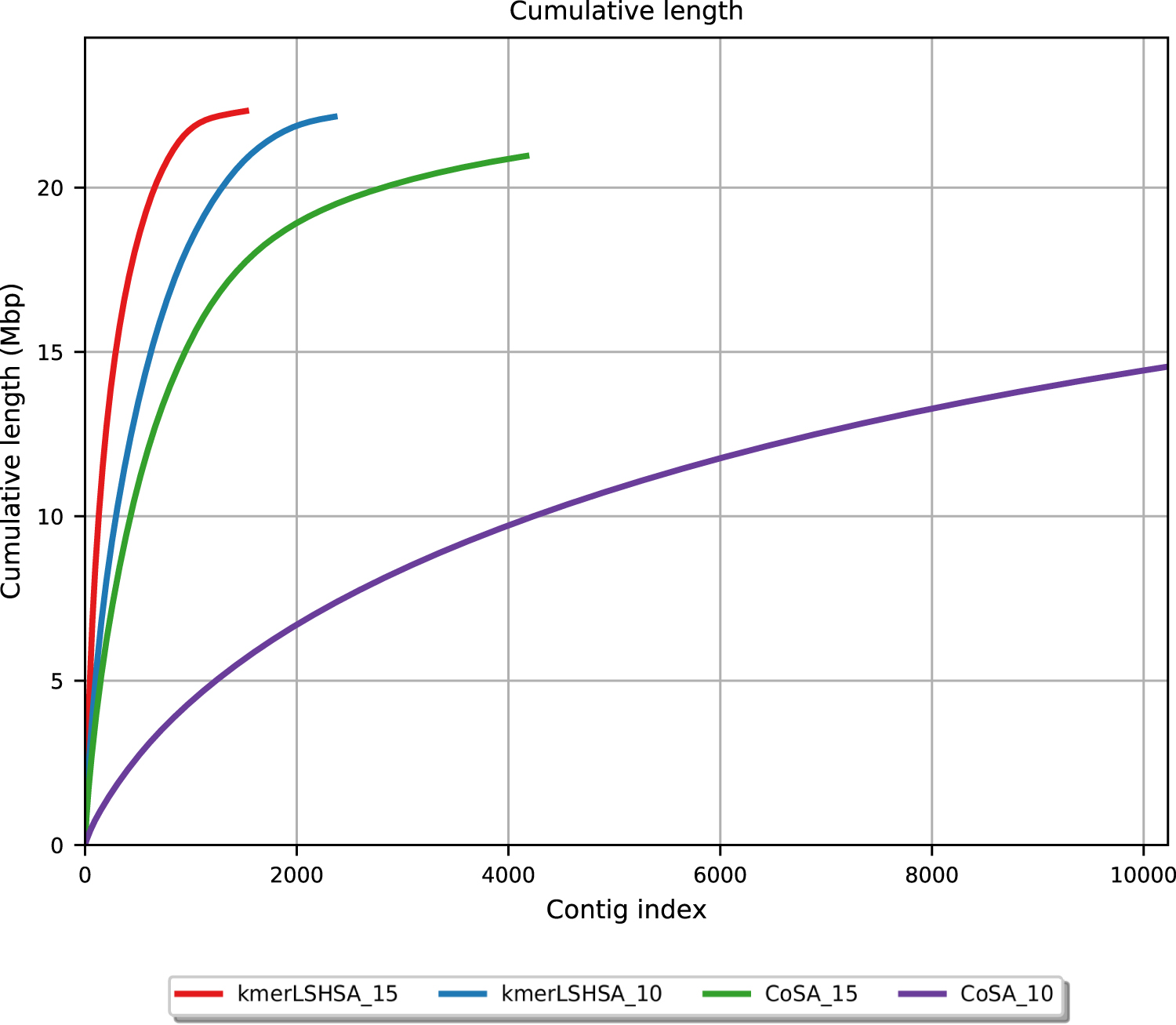
Cumulative length of the contigs generated by kmerLSHSA and CoSA on the two simulated data sets, which contain 15 and 10 samples in each of the two groups, respectively. The contigs were first sorted in the decreasing order of their lengths, and the cumulative length (y-axis) of the first i contigs was depicted as a function of the contig index i. The kmerLSHSA approach generated fewer but longer contigs than CoSA on both simulated data sets. kmerLSHSA_15 represents the performance by kmerLSHSA using 15 samples in each group, and so on.

3.2. Genes derived from kmerLSHSA can be used to build predictive models for host phenotype predictions

We applied kmerLSHSA to real microbiome data sets that were derived from patients with different diseases to test whether kmerLSHSA can produce differential genes useful for building microbiome-based predictive models for host phenotype prediction. Table 2 summaries the genes derived from these microbiome data sets.

Table 2.

Summary of the Predicted Genes and Coabundance Groups

	LC	T2D	NSCLC	RCC
kmerLSHSA
No. of predicted genes	116,972	17,808	3804	5656
No. of CAGs	7259	2508	860	483
CoSA
No. of predicted genes	157,424	296,871	4854	11,287
No. of CAGs	13,793	40,596	1808	2144
Genes
No. of predicted genes	5,627,183	4,013,623	4,044,510	3,914,940
No. of differential genes	651,813	12,123	627	1978
No. of CAGs	1,913,052	808,739	956,237	542,007

CAGs, coabundance groups of genes; CoSA.

The choice of different ML algorithms (and their parameter settings) as well as the type of input features has high impact on the performance of the resulting predictive models. Here, we attempt to compare the impact of the data type (the input to the ML algorithms) on the performance of predictive models. Therefore, we used the same ML protocol and the nested cross-validation where the inner cross-validation was used to choose the ML algorithm and hyperparameters that gave the most accurate predictive models (see Section 2). We compared the effectiveness of four different inputs for building ML models: CAGs from kmerLSHSA, CAGs from CoSA, CAGs from all genes assembled from metagenomes [Genes (CAGs)], and the species identified from metagenomes [denoted as Species (All)].

To prevent potential information leaks and for fair comparison, we used only the CAGs from kmerLSHSA and CoSA that are differential between the two groups using 80% of the samples (randomly selected for training), so features that were only found to be differential (p < 0.01) because of the 20% test samples were excluded from the training of the models. Similarly, for Genes and Species, we applied the same step to select CAGs and Species that are differential between the two groups using 80% of the samples, resulting in two additional types of inputs to ML: Genes (differential) and Species (differential), for a total of six.

Figure 3 summarizes the performance of the predictive models using the different data types. It shows that using CAGs from subtractive assemblies (kmerLSHSA and CoSA) as the input resulted in more accurate predictive models compared with using CAGs from all assembled genes (Genes) and the species abundances (Species) as input. In addition, kmerLSHSA outperformed CoSA, especially for T2D and NSCLC. For NSCLC, CoSA outperformed Genes and Species, but its performance was still rather poor. Using CAGs from kmerLSHSA improved the model significantly, resulting in much more accurate predictive models with comparable AUC as the predictive models for other diseases.

FIG. 3.

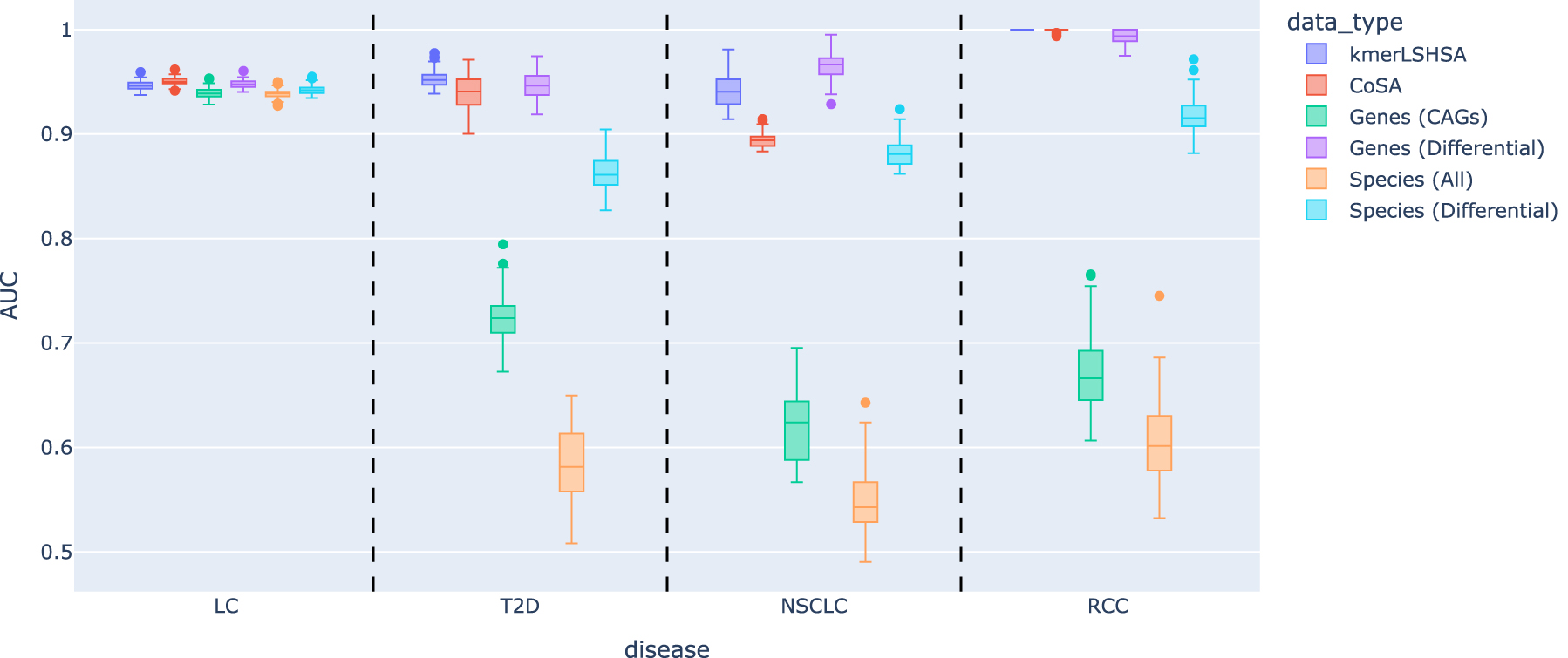
Evaluation of the performance of predictive models using different data types as the inputs. Except for the input data type, all the other settings were kept the same for all the experiments. We conducted a total of 100 replications of training and testing to estimate the variance of the performance; in each iteration, a different splitting of the data into training and test sets was applied. AUC, area under the ROC curve; LC, liver cirrhosis; NSCLC, nonsmall-cell lung cancer; RCC, renal cell carcinoma; T2D, type 2 diabetes.

Using Genes (CAGs) typically resulted in predictive models with poor performance, indicating the challenge imposed by the large number of CAGs to the feature selection. Using statistical tests to select the differential features improves the ML algorithms greatly, resulting in more accurate predictive models [see the performances of Genes (differential)].

Using CAGs from kmerLSHSA as the features resulted in models that have comparable predictive power as the models using differential genes selected from all genes assembled from the microbiome data sets, indicating that kmerLSHSA was able to effectively identify differential genes for downstream analyses, whereas it is much faster than the all-gene-based approach (see Table 3). Using Species resulted in worst predictors across all diseases, and our result is consistent with a previous study that showed using genes as features generally resulted in better predictive models than using species as the features (Le Goallec et al., 2020).

Table 3.

Summary of the Running Time (Minutes) Comparison Between kmerLSHSA and Genes for the Liver Cirrhosis Data Sets

Steps	kmerLSHSA	Genes
Extraction of differential reads	6924	–
Assembly	97	3354
Gene prediction	1	333
Removal of redundant genes (cd-hit)	—	11,687
Mapping	932	25,922
Total	7954	41,296

We examined the combination of ML algorithm and feature selection that gave the best predictive models. The results show that there was no single ML approach and feature algorithm that outperformed others for different data types and different diseases. However, as Figure 4 shows, when CAGs from kmerLSHSA and CoSA were used as the inputs, SVM with L1 feature selection often resulted in the most accurate predictors for LC (Fig. 4a), T2D (Fig. 4b), and RCC (Fig. 4d). For NSCLC, RF with L1 feature selection was the top performer (Fig. 4c). For comparison, the best performing ML and feature selection algorithm varied more when other data types were used as the inputs.

FIG. 4.

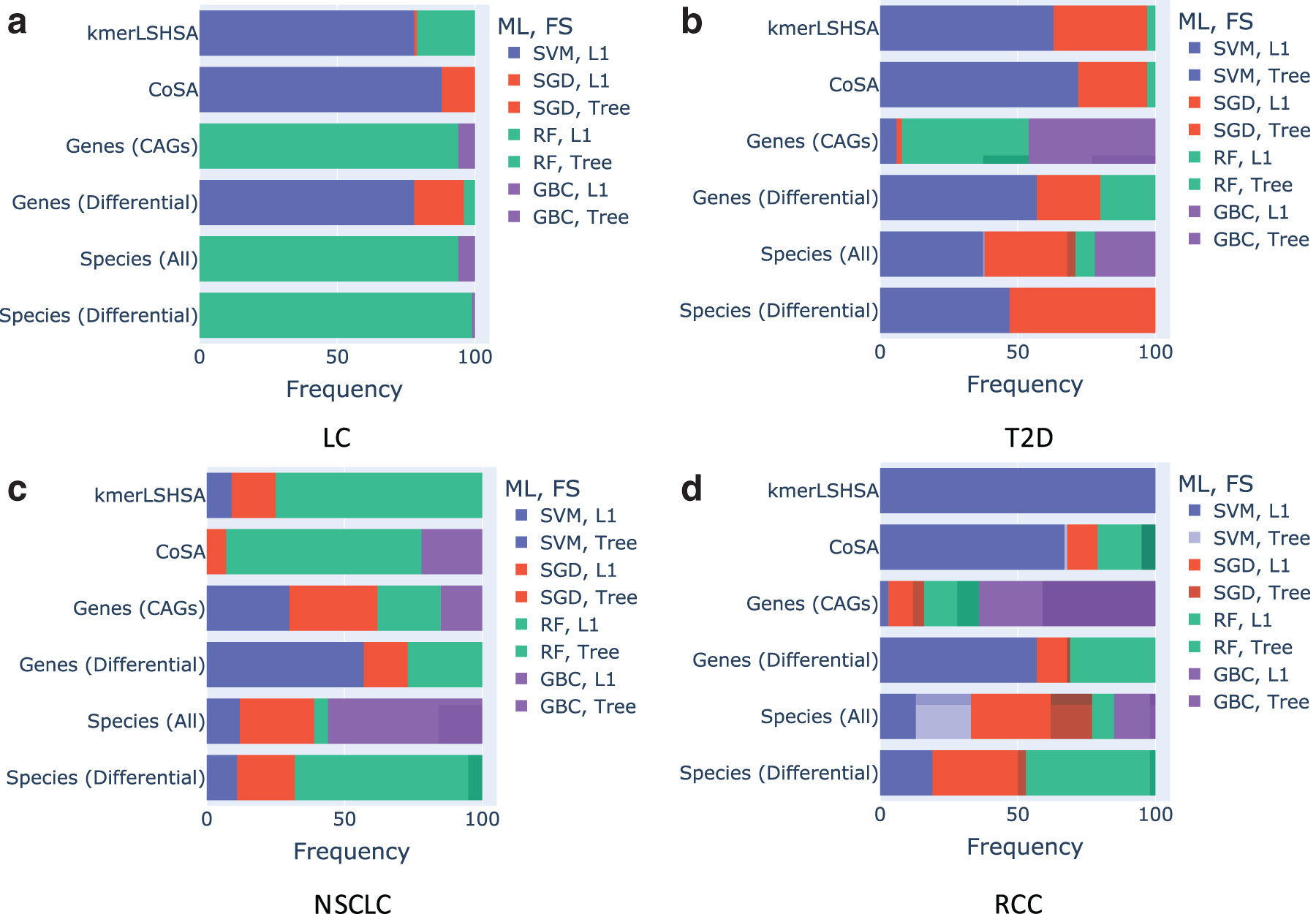
Frequency of different combinations of chosen ML algorithm and feature selection that led to the best predictive models for the different types of inputs for each disease. ML, machine learning. (a)–(d) are for different diseases LC, T2D, NSCLC and RCC, respectively.

Table 3 gives the running times for the different steps in kmerLSHSA and the conventional all-gene-based approach and their overall running time, using the experiments on the LC data sets as an example. All the computations were performed on a server with 12-core Intel Xeon E5-2680 v3 CPUs and 512 GB of RAM. The comparative studies show that although kmerLSHSA has an extra step for the reads subtraction, it gains its advantage by saving the computational time in the subsequent steps as it only uses a much smaller collection of potential differential genes in those steps.

3.3. kmerLSHSA generates a compact and effective collection of genes for building predictive models

We already showed that using CAGs from kmerLSHSA outperformed CAGs from CoSA and all genes (in which the best subset of CAGs was selected using one of the feature selection approaches in the cross-validation). Here, we consider a different question: as the collection of CAGs from kmerLSHSA is already compact, does any subset of CAGs provide a comparable discriminating power for building predictive models as the selected subset of CAGs by feature selection? To address this question, we randomly selected a subset of CAGs (of the same size as the number of samples for each disease) and used it as the input (without feature selection) for building predictive models.

Figure 5 summarizes the performance. Unsurprisingly, because of their large feature space, predictive models using randomly selected features from Gene (CAGs) and Species (All) gave random predictions for T2D, NSCLC, and RCC, respectively. We note that because we used the nested cross-validation to evaluate the performance of predictive models, the reported performance of some models using randomly selected features could be worse than random guess. By contrast, using CAGs from subtractive assembly approaches, especially our new approach kmerLSHSA, resulted in much better predictive models for these diseases. We note that for LC data set, the microbiomes of patients with LC are so different from the healthy controls such that using any randomly selected small collection of genes or species resulted in good predictors.

FIG. 5.

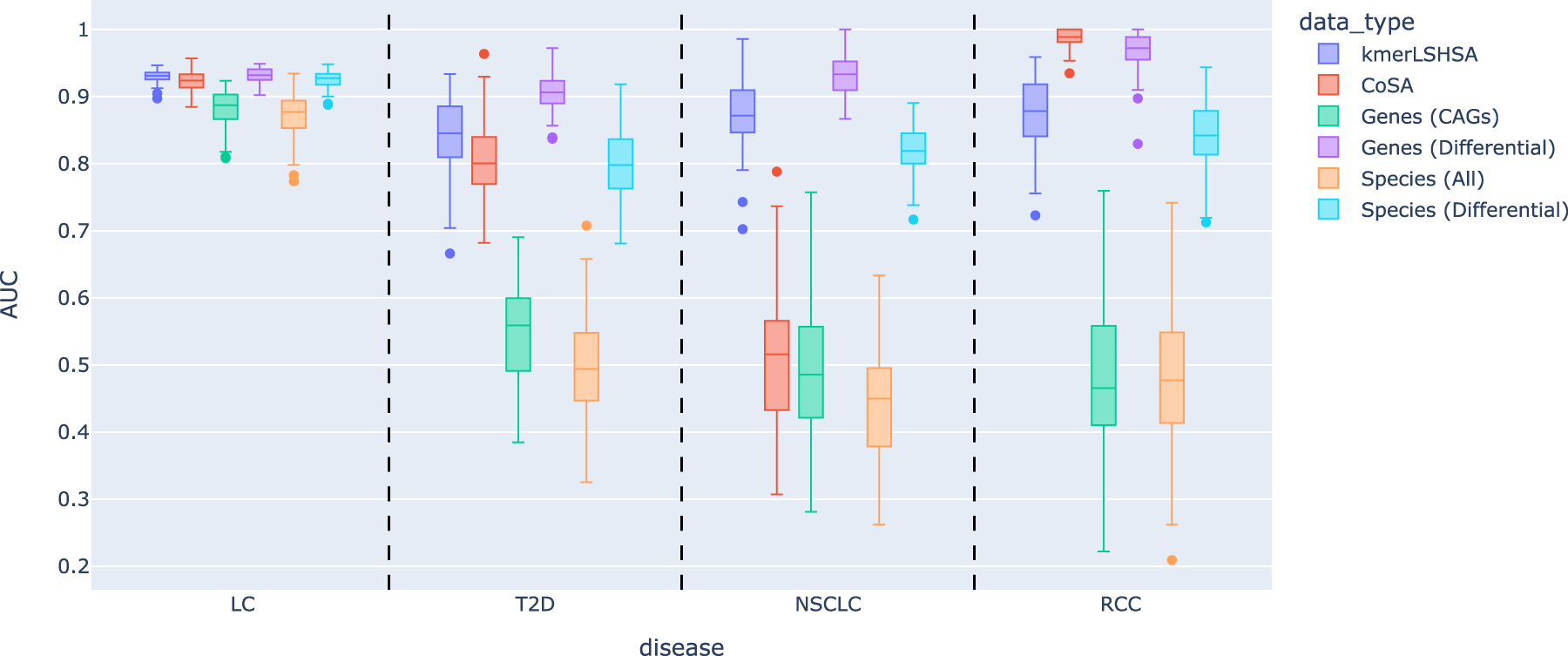
The performances of the predictors with randomly selected features (genes or species). The box plots show the mean and standard deviation of AUC on 100 models built from the replicated training/testing experiments.

4. Discussion

In this article, we presented an improved subtractive assembly approach kmerLSHSA using k-mers clustering for comparative analysis. The key idea of the subtractive assembly approach is to capture the differential reads coming from the differentially enriched genes/genomes before the analysis such as assembly, binning, and gene prediction. Considering the complex microbial community in the real world, it is important to capture the genomes/genes showing low abundances but consistently differences, which may play an important role related with a human disease, as demonstrated in the results on real microbiome data sets derived from patients with different diseases.

The kmerLSHSA approach exploits the LSH technique for clustering k-mers based on their abundance vectors. Because of the huge number of k-mers, it is computationally expensive to directly apply the conventional clustering algorithms such as k-means or hierarchical clustering. To cluster billions of k-mers within a feasible time, the number of hash functions for LSH was determined by the log value of the number of k-mers. The LC data set contains 6 billions of k-mers, which was clustered into 11 millions of kCAGs with the cosine similarity threshold of 0.85.

If a lower similarity threshold is used, the number of clusters (kCAGs) will be further reduced. However, at the same time, some false positives (in this case nondifferential k-mers) may be grouped in the differential kCAGs. Tests on simulated data sets show that reads from the genomes with minor abundance differences between two groups could be successfully extracted with high (0.85) similarity threshold.

As shown in Figure 3, the predictive models using CAGs from kmerLSHSA reached higher AUC compared with the prior version of subtractive assembly and all genes/species assembled from metagenomes. In particular, the LC data set contains many differential genes compared with other data sets (Table 2) that very accurate predictive models could be learned regardless of what features were used. Even though the differences between the median AUC were small for different input data types, compared with the data sets from other diseases, the model of kmerLSHSA still reached the highest AUC (0.951) among all the methods.

In contrast, for NSCLC, the microbiomes of the two groups had much smaller differences (as reflected in the small number of differential genes), and the input data types had much bigger impact on the performance of the predictive models; in this case, only two models reached the AUC over 0.9 (kmerLSHSA and Genes [differential]). These results showed that regardless of the input data sets, kmerLSHSA reported the genes that could serve as good features for building predictive models for phenotype prediction.

We used a nested cross-validation approach and feature selection that regulated the number of features to select for building models to avoid overfitting. However, the generalization of our predictive models (in fact any microbiome-based predictive models) could be relatively low; one needs to be cautious when applying microbiome-based predictive models to new samples, due to the large variation and heterogeneity of microbiome data, as well as the potential confounding factors that could cause the microbiome differences and were not considered properly when building the models (Poussin et al., 2018; Wirbel et al., 2021). Nevertheless, this study demonstrated the importance of curating input features for building predictive models.

Although kmerLSHSA is designed for subtractive assembly, the k-mers clustering result could be used for other purposes. One direction is to check whether the kCAGs can be directly used as markers for studying the differences of microbiomes between groups. Another possible application is to use kCAGs for binning the reads to improve assembly of individual genomes, when multiple microbiome data sets are available (e.g., time course microbiome data). Finally, we expect that the implementation strategies we developed (such as the nested LSH) would be useful for clustering other type of large data sets.

Footnotes

Authors' Contributions

W.H. was in charge of conceptualization, data curation, formal analysis, methodology, software, visualization, writing—original draft, and writing—review and editing. H.T. contributed to conceptualization, formal analysis, methodology, writing—original draft, and writing—review and editing. Y.Y. was involved in conceptualization, formal analysis, funding acquisition, project administration, supervision, writing—original draft, and writing–review and editing.

Acknowledgment

The authors thank Dr. Qin Zhang from Indiana University for helpful discussion of LSH.

Author Disclosure Statement

The authors declare they have no competing financial interests.

Funding Information

This study was supported by NIH grant 1R01AI143254 and NSF grant 2025451.

References

Aitchison

1982. The statistical analysis of compositional data. J. R. Stat. Soc. Ser. B (Methodol). 44, 139–160.

Altamirano-Barrera

, Uribe

, Chávez-Tapia

N.C.

, et al. 2018. The role of the gut microbiota in the pathology and prevention of liver disease. J. Nutr. Biochem. 60, 1–8.

Andoni

, and Indyk

2006. Near-optimal hashing algorithms for approximate nearest neighbor in high dimensions, 459–468. 2006 47th Annual IEEE Symposium on Foundations of Computer Science (FOCS'06). IEEE.

Charikar

M.S.

2002. Similarity estimation techniques from rounding algorithms, 380–388. Proceedings of the Thirty-Fourth Annual ACM Symposium on Theory of Computing.

Dai

, Coker

O.O.

, Nakatsu

, et al. 2018. Multi-cohort analysis of colorectal cancer metagenome identified altered bacteria across populations and universal bacterial markers. Microbiome. 6, 1–12.

Deorowicz

, Kokot

, Grabowski

, et al. 2015. KMC 2: Fast and resource-frugal k-mer counting. Bioinformatics. 31, 1569–1576.

Fritz

, Hofmann

, Majda

, et al. 2019. Camisim: Simulating metagenomes and microbial communities. Microbiome. 7, 1–12.

, Niu

, Zhu

, et al. 2012. Cd-hit: Accelerated for clustering the next-generation sequencing data. Bioinformatics. 28, 3150–3152.

Haase

, Haghikia

, Wilck

, et al. 2018. Impacts of microbiome metabolites on immune regulation and autoimmunity. Immunology. 154, 230–238.

10.

Han

, Wang

, and Ye

2017. A concurrent subtractive assembly approach for identification of disease associated sub-metagenomes, 18–33. International Conference on Research in Computational Molecular Biology. Springer.

11.

Han

, and Ye

2018. A repository of microbial marker genes related to human health and diseases for host phenotype prediction using microbiome data, 236–247. BIOCOMPUTING 2019: Proceedings of the Pacific Symposium. World Scientific.

12.

Jie

, Xia

, Zhong

S.L.

, et al. 2017. The gut microbiome in atherosclerotic cardiovascular disease. Nat. Commun. 8, 1–12.

13.

Kim

C.Y.

, Lee

, Yang

, et al. 2021. Human reference gut microbiome catalog including newly assembled genomes from under-represented Asian metagenomes. Genome Med. 13, 1–20.

14.

Kokot

, Długosz

, and Deorowicz

2017. KMC 3: Counting and manipulating k-mer statistics. Bioinformatics. 33, 2759–2761.

15.

Langmead

, and Salzberg

S.L.

2012. Fast gapped-read alignment with Bowtie 2. Nat. Methods. 9, 357–359.

16.

Le Goallec

, Tierney

B.T.

, Luber

J.M.

, et al. 2020. A systematic machine learning and data type comparison yields metagenomic predictors of infant age, sex, breastfeeding, antibiotic usage, country of origin, and delivery type. PLoS Comput. Biol. 16, e1007895.

17.

, Luo

, Liu

C.M.

, et al. 2016. Megahit v1. 0: A fast and scalable metagenome assembler driven by advanced methodologies and community practices. Methods. 102, 3–11.

18.

, Andersen

D.G.

, Kaminsky

, et al. 2014. Algorithmic improvements for fast concurrent cuckoo hashing. Proceedings of the 9th ACM European Conference on Computer Systems (EuroSys).

19.

Lloyd-Price

, Arze

, Ananthakrishnan

A.N.

, et al. 2019. Multi-omics of the gut microbial ecosystem in inflammatory bowel diseases. Nature. 569, 655–662.

20.

, Breitwieser

F.P.

, Thielen

, et al. 2017. Bracken: Estimating species abundance in metagenomics data. PeerJ Comput. Sci. 3, e104.

21.

Marçais

, DeBlasio

, Pandey

, et al. 2019. Locality-sensitive hashing for the edit distance. Bioinformatics. 35, i127–i135.

22.

Melsted

, and Pritchard

J.K.

2011. Efficient counting of k-mers in DNA sequences using a bloom filter. BMC Bioinformatics. 12, 1–7.

23.

Nejman

, Livyatan

, Fuks

, et al. 2020. The human tumor microbiome is composed of tumor type–specific intracellular bacteria. Science. 368, 973–980.

24.

, and Zhang

2020. Deepmicro: Deep representation learning for disease prediction based on microbiome data. Sci. Rep. 10, 1–9.

25.

Ondov

B.D.

, Starrett

G.J.

, Sappington

, et al. 2019. Mash screen: High-throughput sequence containment estimation for genome discovery. Genome Biol. 20, 1–13.

26.

Ondov

B.D.

, Treangen

T.J.

, Melsted

, et al. 2016. Mash: Fast genome and metagenome distance estimation using minhash. Genome Biol. 17, 1–14.

27.

Pedregosa

, Varoquaux

, Gramfort

, et al. 2011. Scikit-learn: Machine learning in Python. J. Mach. Learn. Res. 12, 2825–2830.

28.

Poore

G.D.

, Kopylova

, Zhu

, et al. 2020. Microbiome analyses of blood and tissues suggest cancer diagnostic approach. Nature. 579, 567–574.

29.

Poussin

, Sierro

, Boué, et al. 2018. Interrogating the microbiome: Experimental and computational considerations in support of study reproducibility. Drug Discov. Today. 23, 1644–1657.

30.

Qin

, Li

, Raes

, et al. 2010. A human gut microbial gene catalogue established by metagenomic sequencing. Nature. 464, 59–65.

31.

Qin

, Li

, Cai

, et al. 2012. A metagenome-wide association study of gut microbiota in type 2 diabetes. Nature. 490, 55–60.

32.

Qin

, Yang

, Li

, et al. 2014. Alterations of the human gut microbiome in liver cirrhosis. Nature. 513, 59–64.

33.

Rho

, Tang

, and Ye

2010. FragGeneScan: Predicting genes in short and error-prone reads. Nucleic Acids Res. 38, e191.

34.

Routy

, Le Chatelier

, Derosa

, et al. 2018. Gut microbiome influences efficacy of pd-1–based immunotherapy against epithelial tumors. Science. 359, 91–97.

35.

Silva

, Brunner

, and Tschurtschenthaler

2021. Microbiota and colorectal cancer: From gut to bedside. Front. Pharmacol. 2716.

36.

Soto

J.E.

, Krohmer

, Hernández

, et al. 2019. Hardware acceleration of k-mer clustering using locality-sensitive hashing, 659–662. 2019 22nd Euromicro Conference on Digital System Design (DSD). IEEE.

37.

Wang

, and Jia

2016. Metagenome-wide association studies: Fine-mining the microbiome. Nat. Rev. Microbiol. 14, 508–522.

38.

Wang

, Shen

H.T.

, Song

, et al. 2014. Hashing for similarity search: A survey. arXiv preprint arXiv:1408.2927.

39.

Wang

, Li

, and Tang

2018. mscrush: Fast tandem mass spectral clustering using locality sensitive hashing. J. Proteome Res. 18, 147–158.

40.

Wang

, Doak

T.G.

, and Ye

2015. Subtractive assembly for comparative metagenomics, and its application to type 2 diabetes metagenomes. Genome Biol. 16, 1–15.

41.

Wang

X.W.

, and Liu

Y.Y.

2020. Comparative study of classifiers for human microbiome data. Med. Microecol. 4, 100013.

42.

Wirbel

, Zych

, Essex

, et al. 2021. Microbiome meta-analysis and cross-disease comparison enabled by the SIAMCAT machine learning toolbox. Genome Biol. 22, 1–27.

43.

Zeller

, Tap

, Voigt

A.Y.

, et al. 2014. Potential of fecal microbiota for early-stage detection of colorectal cancer. Mol. Syst. Biol. 10, 766.

44.

Zhang

, Pell

, Canino-Koning

, et al. 2014. These are not the k-mers you are looking for: Efficient online k-mer counting using a probabilistic data structure. PLoS One. 9, e101271.

45.

Zhang

, Zhang

, Jia

, et al. 2015. The oral and gut microbiomes are perturbed in rheumatoid arthritis and partly normalized after treatment. Nat. Med. 21, 895–905.

46.

Zhao

, Zhang

, Ding

, et al. 2018. Gut bacteria selectively promoted by dietary fibers alleviate type 2 diabetes. Science. 359, 1151–1156.

Locality-Sensitive Hashing-Based k-Mer Clustering for Identification of Differential Microbial Markers Related to Host Phenotype

Abstract

1. Introduction

2. Methods

2.1. Overview of kmerLSHSA

2.2. Building k-mer abundance profiles

2.3. Generating kCAG by LSH

2.4. Subtractive assembly

2.5. Inference of microbial markers using ML approaches

2.5.1. Gene abundance quantification and inference of gene CAGs

2.5.2. Feature selection and ML algorithms

2.6. Data sets

2.7. Availability of the program and data

3. Results

3.1. Evaluation of kmerLSHSA using simulated data sets

3.2. Genes derived from kmerLSHSA can be used to build predictive models for host phenotype predictions

3.3. kmerLSHSA generates a compact and effective collection of genes for building predictive models

4. Discussion

Footnotes

Authors' Contributions

Acknowledgment

Author Disclosure Statement

Funding Information

References