Sage Journals: Discover world-class research

Abstract

Recurrent whole genome duplication and the ensuing loss of redundant genes—fractionation—complicate efforts to reconstruct the gene orders and chromosomes of the ancestors associated with the nodes of a phylogeny. Loss of genes disrupts the gene adjacencies key to current techniques. With our RACCROCHE pipeline, instead of starting with the inference of short ancestral segments, we suggest delaying the choice of gene adjacencies while we accumulate many more syntenically validated generalized (gapped) adjacencies. We obtain longer ancestral contigs using maximum weight matching (MWM). Similarly, we do not construct chromosomes by successively piecing together contigs into larger segments, but rather compile counts of pairwise contig co-occurrences on the set of extant genomes and use these to cluster the contigs. Chromosome-level contig assemblies for a monoploid genome emerge naturally at each node of the phylogeny and the contigs then can be ordered along the chromosome. Sampling alternative MWM solutions, visualizing heat maps, and applying gap statistics allow us to estimate the number of chromosomes in the reconstruction. We introduce several measures of quality: length of contigs, continuity of contig structure on successive ancestors, coverage of the extant genome by the reconstruction, and rearrangement relations among the inferred chromosomes. The reconstructed ancestors are visualized by painting the ancestral projections on the descendant genomes. We submit genomes drawn from a broad range of monocot orders to our pipeline, confirming the tetraploidization event “tau” in the stem lineage between the alismatids and the lilioids. We show additional applications to the Solanaceae and to four Brassica genomes, producing evidence about the monoploid ancestor in each case.

1. Introduction

The known flowering plants all have whole genome duplication and triplication events (WGD and WGT, respectively) in their evolutionary history since divergence from the last common ancestor of all extant angiosperms (except Amborella trichopoda [Amborella Genome Project, 2013] and Aristolochia fimbriata [Qin et al., 2021]). Immediately subsequent to WGDs and WGTs, genomes undergo a drawn-out and extensive loss of redundant genes. Fractionation, the process of duplicate loss in these polyploids, effectively scrambles gene order and disrupts many if not most preduplication/triplication ancestral adjacencies. This long history of WGD and WGT events followed by fractionation in the lineages of plants makes ancestral genome reconstruction challenging, because methods relying on conserved gene adjacencies tend to break down. For example, duplication of a chromosomal region containing genes ordered 1–2–3–4–5–6–7 may result in gene orders 1–3–4–6 and 2–4–5–7 in the descendant chromosomes, with only one of six gene adjacencies conserved after fractionation. The situation is compounded if there are several WGD or WGT events in the evolutionary history of extant genomes. The consequences of WGD or WGT fractionation processes are superimposed on a background of gene family expansion through tandem duplication and other mechanisms, and loss of genes from species for which they are no longer essential.

Further disrupting adjacencies, extensive genome rearrangements involving chromosome segments of size ranging from kilobases to many megabases, are prevalent in plant genomes. In addition, chromosome fissions and fusions are widespread (Mayrose and Lysak, 2021). After WGD and WGT, fusions tend to be numerous in many plant lineages, leading to a wide range of number of chromosomes among genomes in the same family and even in the same genus.

We have developed a pipeline for ancestral plant genome inference, RACCROCHE, Reconstruction of AnCestral COntigs and CHromosomEs (Xu et al., 2021a). The new strategy implemented in our approach combines seven fundamental components: 1.

The replacement of the traditional selection of 1–1 orthologs among input genomes, as a first step, by the identification of many-to-many correspondences among gene families of limited size within these genomes.

The use of generalized adjacencies (Xu and Sankoff, 2008; Yang and Sankoff, 2010; Gagnon et al., 2012), or any pair of genes within a chromosomal region of a specified length, instead of just immediately adjacent genes or anchor gene pairs separated by a specified maximum number of intervening genes.

These first two components avoid premature decisions on which orthologies and which adjacencies should be incorporated in the final reconstruction, in contrast to approaches that insist on making these decisions early in the reconstruction process, for example, Perrin et al. (2015).

The compilation of oriented candidate adjacencies at each of the ancestral nodes of a given binary branching tree phylogeny using a “multiple support” criterion—that such an adjacency must be evidenced in genomes in two or three of the subtrees connected by this node, not just one or none.

The large set of these candidates is then resolved, at each node, by maximum weight matching (MWM) to give a relatively small optimally compatible subset, which ipso facto defines linearly (or circularly) compatible “contigs” of the ancestral genomes to be constructed, thus avoiding the branching segments that plague other methods (Tannier et al., 2020).

A local sequence matching, satisfying proximity and contiguity conditions, of each contig on all of the chromosomes of the input genomes. This step includes the construction of a total chromosomal co-occurrence matrix of contigs belonging to each ancestral node. A second matrix, of correlations of co-occurrence scores of pairs of contigs over all other contigs, is also calculated.

A clustering applied to the co-occurrence matrix or the co-occurrence correlation matrix. This is then decomposed into chromosomal sets of contigs, with the aid of a heat map comparison of the contigs as organized by the clustering. Within each contig, the order of the genes is already predetermined by the MWM step. Ordering the contigs along the chromosomes is carried out by a linear ordering algorithm. The assignment and ordering of contigs to construct entire chromosomes, and not just a collection of small regions, are an advance over previous methods. Corresponding chromosomes in different ancestral genomes can be identified by similar contigs they contain.

The use of gap statistics to estimate the number of chromosomes when this is not clear from the heat map. This may require multiple samples of MWM solutions.

The reconstructed ancestral contig assemblies are then mapped back to the input genomes, to infer chromosomal rearrangements that occurred along each branch of the species tree linking ancestral and extant genomes.

We provide an evaluation of the reconstruction in terms of the sizes of the ancient chromosomal fragments found, the coherence (or continuity) between adjacent ancestral genomes, the coverage of the ancestors when mapped to extant genomes, and the “choppiness” of this mapping in terms of ancestor–descendant rearrangement.

There has been much recent work on the reconstruction of ancestral plant genomes (Zheng et al., 2013; Badouin et al., 2017; Murat et al., 2017; Avdeyev et al., 2020; Rubert et al., 2020; Zhao et al., 2021); on the computational side most of this has been based on common gene adjacencies in extant genomes, as summarized in structures such as sets of species trees and contiguous ancestral regions (CARs) (Anselmetti et al., 2018). The latter terminology, introduced successfully in the context of mammalian genomes by Ma et al. (2006), where there are no polyploidizations since the common ancestor, and then taken over to plant genomics (Chauve and Tannier, 2008; Badouin et al., 2017; Rubert et al., 2020), applies to a series of methods of which a recent improved exemplar is proCARs (Perrin et al., 2015). We will show that in the case of flowering plants, the avoidance of propagated error due to premature selection of gene adjacencies in RACCROCHE allows the accurate recovery of more of the ancestral genome than proCARs.

Section 2 of this article sets out the main features and procedures of the algorithm. The RACCROCHE pipeline is applied to the reconstruction of four monocot ancestors in a phylogeny relating the six extant monocot plant genomes in Section 3. These include Acorus americanus (sweet flag) in the sister lineage to all other extant monocots (Acorales), Spirodela polyrhiza (duckweed) from the order Alismatales, Dioscorea rotundata (yam) from the order Dioscorales, Asparagus officinalis (garden asparagus) from the order Aspargales, Ananas comosus (pineapple) from the order Poales, and Elaeis guineensis (African oil palm) from the order Arecales. We evaluate the reconstruction, examining the sizes of the chromosomal fragments found, the coherence between successive ancestral genomes, the coverage of the ancestors when mapped to extant genomes, and the “choppiness” of this mapping in terms of ancestor–descendant rearrangement. We use gap statistics to confirm the number of chromosomes already evident in the heat maps.

To explore the general utility of RACCROCHE, it is applied to two additional data sets. The first data set contains six species from the family Solanaceae (Section 4): Solanum tuberosum (potato), Solanum lycopersicum (tomato), Solanum melongena (eggplant), Capsicum annuum (pepper), Nicotiana tabacum (tobacco), and Petunia hybrida (petunia).

Our use of MWM ensures that each gene family appears at most once in a reconstructed ancestor. The effect of this is that our reconstructed ancestor is a monoploid version of that genome (Xu et al., 2021b), which may or may not be the same as the haploid representation. Thus we may apply RACCROCHE to a genome that has undergone one or more WGDs or WGTs, to try to recover the underlying monoploid structure before polyploidization. In Section 5, RACCROCHE is applied to four species in the WGD- or WDT-rich family of Brassicaceae: Brassica oleracea, Brassica nigra, Brassica rapa, and Brassica napus. For these species, RACCROCHE reconstructed the ancestors without reference to a predefined phylogenetic relationship of the species. The idea was to see which, if any, of the genomes contains evidence of an earlier monoploid ancestor.

Section 6 summarizes our conclusions and outlines some future directions for research and refinement of our methods.

2. Methods

The RACCROCHE pipeline consists of nine major stages in a cascade manner as depicted in Figure 1.

FIG. 1.

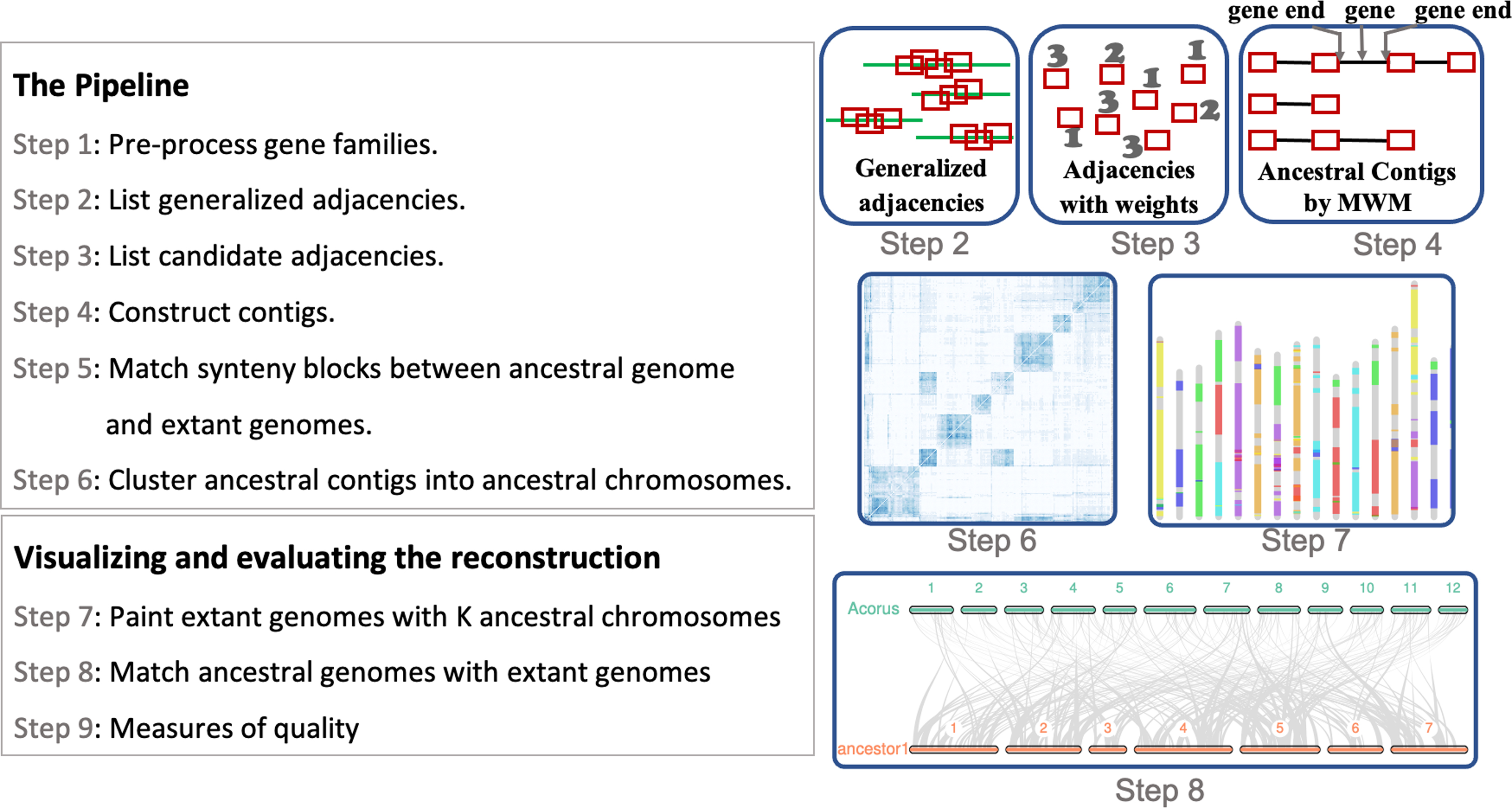
Nine stages of the RACCROCHE procedure for ancestral genome reconstruction.

The important parameters are discussed first in Section 2.1.

2.1. Input

The input to RACCROCHE consists of N annotated extant genomes related to a given unrooted binary branching phylogeny, and a number of parameters, including

W: window size to include generalized as well as immediate adjacencies,

NF: largest total gene family size allowed in ortholog grouping in all extant genomes,

NG: largest gene family size allowed in any one genome,

NC: the number of longest contigs in ancestral genomes to be matched to extant genomes,

K: the desired number of chromosomes for each ancestor, and

DIS: the maximum distance between two adjacent genes in an extant genome to be matched with adjacent genes in an ancestral contig.

We set $N F \leq N \times N G$ to avoid the loss of generality.

2.2. The pipeline

2.2.1. Step 1: Preprocess gene families

Starting with syntenically validated orthogroups, or gene families, constructed from $\frac{1}{2} (N^{2} + N)$ between-genome and self-comparison sets of pairwise SynMap synteny blocks, RACCROCHE collects all genes that are syntenically homologous to at least one other gene in the family, then retains only those families with at most NF of members and at most NG members in any particular genome.

The use of syntenically validated adjacencies only, restricted to genes appearing in synteny blocks identified by the comparison of some pair of the descendant genomes, avoids generating huge gene families and astronomical number of adjacencies not reflective of the ancestor.

As an optional second “redistribution” step, all families with more than NF members or more than NG members in any particular genome are flagged. Then the construction of the families is repeated, with the restriction that no gene can be recruited to a family by virtue only of a similarity of less than some threshold homology level $θ$ to a gene already in the family. The intent is to break up large families held together by a few weak links, and thus to retrieve some better supported smaller families.

2.2.2. Step 2: List generalized adjacencies

For each extant genome, RACCROCHE compiles all generalized adjacencies, that is, representatives of two gene families, occurring within a window of a preset size, W, in the order of genes on a chromosome. The adjacencies are oriented by the DNA strand(s) containing the two genes, so that we can distinguish the two ends of each gene, and identify which ends are involved in the adjacency.

2.2.3. Step 3: List candidate adjacencies

For each ancestral tree node, allow only adjacencies in occurring in at least two of the three subtrees connected by a branch incident to that node as candidates to be adjacencies in the corresponding ancestral genome. Occurrence in a subtree means occurrence in at least one of the extant genomes in that subtree.

2.2.4. Step 4: Construct contigs

A MWM algorithm is applied to the candidate adjacencies (weighted 2 or 3 according to whether they occur in two or three subtrees) from the last step. The MWM results correspond to the highest weight set of compatible adjacencies, that is, each gene end is matched to at most one other gene end, which automatically defines a set of disjoint contigs of gene families in linear orders for the ancestral genome.

RACCROCHE executes for a single set of $W, N F, N G$ parameters, or for a range of values of W and NG. In the latter case, there is an option, designed to increase coherence among sets of contigs for successive ancestors, that the MWM for any combination of W and NG must be restricted to include all adjacencies already recovered for lesser values of W or NG, insofar as possible. Thus, starting with some small W and NG, we can construct MWM solutions for larger window size and/or larger gene family size, and hence sets of contigs, by incrementing one or the other of the parameters. This comes at the cost of other qualities of the contigs, and will not be discussed further here.

It is possible, however, to have conflicts between $(W, N G - 1)$ and $(W - 1, N G)$ analyses. For example, if adjacencies $(a, b)$ and $(b, c)$ are in the MWM for $(W, N G - 1)$ and $(a, b)$ and $(b, d)$ are in the MWM for $(W - 1, N G)$ , then a matching for $W, G$ cannot be forced to include all matchings from the two previous MWM. To accommodate this possibility, when we restrict the MWM for $(W, N G)$ to include all adjacencies from $(W, N G - 1)$ and $(W - 1, N G)$ , we make an exception for any adjacencies from either that are in potential conflict with adjacencies from the other. Thus $(a, b)$ in the example above might be obligatorily included, but $(b, c)$ and $(b, d)$ would not. Thus the MWM for $(W, N G)$ might include $(b, c)$ or $(b, d)$ , but not both.

2.2.5. Step 5: Match synteny blocks between ancestral genome and extant genomes

For each contig in an ancestral genome, search for locally matched regions to recover synteny blocks in all extant genomes. This process is formally described as follows.

For the ancestor genome, A, computed from a set of extant genomes neighboring $G_{1}, G_{2}, \dots, G_{n}$ , perform the following steps.

Search gene families in descendant genomes.

For every gene family, g, in ancestor A, retrieve six features of this gene family in every extant genome involved in constructing ancestor A. The features of a gene in an extant genome include chromosome ID, start and end chromosomal positions, distance between g to its next adjacent gene, gene family ID labeled in Step 1, and contig ID in A.

Identify ancestral syntenic blocks in descendant genomes.

First, initialize a syntenic block by merging two adjacent genes given a distance threshold DIS: merge two genes, g₁ and g₂, to form a “seed” of a syntenic block if g₁ and g₂ locate the same chromosome, are adjacent to each other, and the distance between them is less than or equal to the distance threshold DIS (i.e., DIS = 1 Mbp). Each ancestral syntenic block is extended from the “seed” by merging flanking gene(s) into the block if the gene(s) satisfies the mentioned three conditions. The extension of a block ends if no flanking gene could be merged into the block.

2.2.6. Step 6: Cluster ancestral contigs into ancestral chromosomes

Clustering of ancestral chromosomes is based on co-occurrence of ancestral contigs of sufficient size on the same chromosomes of extant genomes. First, a co-occurrence matrix is constructed counting the cumulative number of times two different contigs are matched on the same chromosome in one or more extant genomes. Next, a complete-link hierarchical clustering of the contigs is performed in each ancestral genome, based on the correlation of co-occurrence. The hierarchical cluster is decomposed either automatically (e.g., with a cutoff level or with a cluster size criterion) or with some biologically motivated manual intervention into a preset number K of chromosomes. See Section 3.2 for an example.

Contigs are ordered by applying the algorithm of linear ordering problem (LOP) (Schiavinotto and Stützle, 2004) based on the count of relative ordering, the number of times each contig appears upstream/downstream of the other contig for every pair of contigs within a cluster.

The clustering and ordering are detailed as the following steps:

Filter the set of blocks longer than a block length threshold.

Count co-occurrence of ancestral contigs on same chromosomes.

Cluster ancestral contigs into ancestral chromosomes according to a distance matrix calculated from co-occurrence.

A distance matrix, dmat, normalized from the co-occurrence matrix, is calculated as $d m a t_{i, j} = - log (\frac{{max}_{f r e q} - m_{i, j}}{{max}_{f r e q}}) .$

This distance matrix is fed into the complete-link clustering algorithm. This can then be composed into K clusters, according to users' definition. The resultant clusters of contigs correspond to ancestral chromosomes and their compositions.

We then replace raw co-occurrence frequencies with another measure of the likely common ancestral chromosome membership of two contigs x and y. This follows the observation, on one hand, of many contig pairs showing low co-occurrence with each other but otherwise having an identical or similar pattern of co-occurrence frequencies with other contigs, whereas, on the other hand, some contig pairs show elevated co-occurrences, despite little similarity between their patterns of co-occurrence with other contigs. To eliminate these anomalies, we use the correlation $r_{x y}$ between the co-occurrence frequencies of x and y with all the other contigs as a clustering criterion. Let $n = n_{c o n t i g s} - 2$ , where $n_{c o n t i g s}$ is the total number of contigs.

The effects of changing to the correlation measure are made clear in examining the formula for Pearson's coefficient of correlation, $r_{x y} = \frac{N C \sum x_{i} y_{i} - \sum x_{i} \sum y_{i}}{\sqrt{N C \sum x_{i}^{2} - {(\sum x_{i})}^{2}} \sqrt{N C \sum y_{i}^{2} - {(\sum y_{i})}^{2}}} .$ (1)

The sums are taken over all NC contigs x, where $i \neq x$ and $j \neq x$ , x_i is the co-occurrence between x and i and y_i is the co-occurrence between y and i.

As discussed in Xu et al. (2021c), by applying Pearson's coefficient of correlation, the covariance of co-occurrence frequencies is normalized and, therefore, the large variability of the data is mitigated. Any scale bias is largely removed because multiplying all the x_i, for example, by the same constant in Eq. (1) has no effect on $r_{x y}$ .

2.2.7. Step 6a: Use of gap statistics to estimate the number of chromosomes when it is not clear from the heat map

Although the heat map itself is often strongly suggestive about the number of clusters existing in the set of contigs, as in the monocot data set we explore in Section 3, with other data it is more ambiguous, as with the Solanaceae analysis in Section 4.

To add a less subjective aspect to this question, we take advantage of the nonuniqueness of the MWM solution for constructing contigs. Although these solutions are within 92%–97% identical by any measure, they lead to heat maps that are often different in many details, and that are suggestive of somewhat different chromosomal structure.

We thus sample a number of MWM solutions, induced by different orders of the input adjacencies. It is computationally quite feasible to take 10 samples. We then calculate the co-occurrence correlation matrix as already described. This in turn serves as input to the gap statistic analyses (Tibshirani et al., 2001).

A plot of the gap stat value of a k-chromosome analysis typically shows a rapid rise for $k = 2, 3, \dots$ until an inflection point where the slope of the increase drops significantly. The last k for which the value increases substantially may be taken as an estimate $\hat{k}$ of the number of chromosomes. Since this typically varies among the MWM samples, we plot all the values on a single graph to find a consensus value of $\hat{k}$ . We introduce a different method for detecting the inflection point, constructing a linear fit to the values for the first few values of k, representing bonafide improvements in the explanatory power of larger k, and a second linear relation to the last few k, representing nonexplanatory overfitting by excessive number of chromosomes. Where the two lines intersect is our proposed estimate of k.

To order the contigs along each chromosome, we proceed as follows.

The relative ordering between every pair of contigs is analyzed. The number of times each contig appears upstream/downstream of other contig is collected into an $N C \times N C$ ordering matrix, C, where the rows and columns are contig IDs from 0 to $N C - 1$ . $c_{i, j}$ represents the number of times contig i occurred in upstream of contig j in the extant chromosomes.

Given the ordering matrix C, the LOP is the problem of finding a permutation $π$ of the column and row indices ${1, \dots, N C}$ , such that the value $f (π) = \sum_{i = 1}^{N C} \sum_{j = i + 1}^{N C} C^{(π (i), π (j))}$ (2)

is maximized (Schiavinotto and Stützle, 2004). In other words, the goal is to find a permutation of the columns and rows of C such that the sum of the elements in the upper triangle is maximized.

By applying a meta-heuristic solver of LOP, Tabu Search (Martí et al., 2012), the solution order corresponds to the ordering/permutation of contigs sorted by their positions along ancestral chromosomes.

These procedures have been validated through simulation studies (Xu et al., 2021c).

2.3. Visualizing and evaluating the reconstruction

2.3.1. Step 7: Painting the extant genomes according to the ancestral chromosomes

Each of the K chromosomes of an ancestor genome is assigned a different color. Each extant genome can then be painted by the colors of an ancestor based on the coordinates of synteny blocks calculated in Step 5. Unpainted regions <1 Mb long between two blocks of the same color are also painted with that color. Although we can establish a general correspondence between the chromosomes of the successive ancestor genomes, the synteny blocks and the painting of the extant genomes will nevertheless depend on which ancestor is used. In general, the immediate ancestor of a genome gives the most easily interpretable painting.

2.3.2. Step 8: Adapting MCScanX to match ancestral genomes with extant genomes

We use MCScanX (Wang et al., 2012) to connect matching parts of each descendant and its immediate ancestor, as well as to calculate the optimal order of chromosomes.

MCScanX requires both gene location and gene sequence to search pairwise synteny. The “genes” in the constructed ancestors, however, are really gene families, each represented by a integer label. For the purposes of MCScanX, we simply choose a member of the gene family, either randomly, or from a descendant of that ancestor.

For viewing purposes, the number of “crossing” lines in the trace diagram should be minimized. MCScanX searches for the ordering of the chromosomes that minimizes this, using a genetic algorithm.

2.3.3. Step 9: Measures of quality

In the construction of the contigs, we count how many gene families and how many candidate adjacencies are incorporated in total by the MWM. We also document details of the contig length distribution, for example, the longest contig and N50.

The coherence between all pairs of contig sets, each set associated with one ancestor, is a more global way of assessing the reconstruction. To be credible, the contigs at one ancestral node should resemble to some extent the contigs at a neighboring ancestor node.

A measure of commonality between two contigs i and j from two ancestors I and J, respectively, is given by $s i m_{i j} = \frac{x_{i j}}{\sqrt{x_{i .} x_{. j}}},$ (3)

where $x_{i .}, x_{. j}$ , and $x_{i j}$ are the number of gene families in contig i, in contig j, and in both contigs, respectively.

Then, calculating the coherence between two tree nodes for the NC longest contigs $c o h e r e n c e_{I J} = \frac{\sum_{i} {max}_{j = 1}^{N C} s i m_{i j},}{N C} .$ (4)

Percent coverage is defined as the percentage that genome G is covered by the synteny block set of ancestor A. It also reflects how closely ancestor A is related to G.

Choppiness of painting in G is quantitatively measured by the number of different colors, T, the number of single-color regions, R, and the number of small stripes, X, on each extant chromosome (Mazowita et al., 2006). T is defined as the sum number of different colors on each chromosome of G minus 1, reflecting how much interchromosomal exchange, such as translocation, there has been; R is defined as the sum number of single-color regions on each chromosome of G and is a measure of how much intrachromosomal movement (e.g., reversals or transpositions) there has been; X is defined as the number of stripes less than a certain threshold size (i.e., 300 Kbp), which we deduct to avoid inflating R. The choppiness measure of painting in G is written as $R - X$ .

3. Reconstruction of Monocot Ancestors

We applied our method to the reconstruction of four monocot ancestors, given six extant monocot plant genomes from A. americanus, S. polyrhiza, D. rotundata, A. officinalis, E. guineensis, and A. comosus. The phylogenetic tree is shown in Figure 2. The divergence time from Ancestor 1 to any of the extant genomes is ∼130 Mya (Givnish et al., 2018). The reconstruction problem is complicated due not only to this lengthy elapsed time, since the early Cretaceous, comparable with that of the early divergence of placental mammals, but also to the occurrence of at least one WGD in every order, and generally two or more.

FIG. 2.

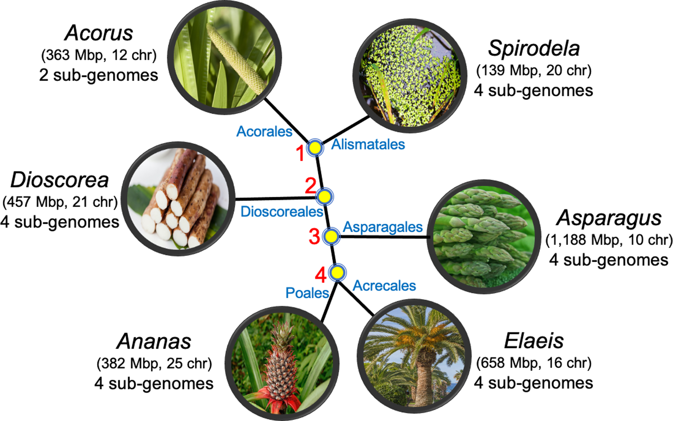
Phylogeny showing relationships among six monocots and their ancestors.

One question we aimed to answer was whether both ancient WGD detected in the extant Dioscorea genome occurred after its branching off the stem lineage to Asparagales, Arecales, and Poales, or whether one of these WGDs occurred earlier, between Ancestors 1 and 2, and is identical to the “tau” event known to affect all these later branching orders.

3.1. Properties of the contig reconstruction

After numerous trials, input parameters that seemed (somewhat subjectively) to balance contig length properties, coherence, and coverage were chosen to be window size $W = 7$ , maximum total family size $N F = 50$ , and within-genome maximum family size $N G = 10$ . Table 1 summarizes the gene content of each of the input genomes, first, syntenically validated genes (i.e., in synteny blocks); second, after removing very large gene families; third, after filtering for within-genome family size; fourth, genes present in a candidate adjacency; and fifth, genes incorporated in the 250 longest contigs for any ancestor.

Table 1.

Number of Genes at Each Step of Building Contigs

	In synteny blocks	In families $< 5000$	In filtered families	In candidate adjacencies	In contigs, after MWM
Acorus	21,308	11,807	11,300	10,189	9649
Spirodela	20,751	8385	8005	7706	7276
Dioscorea	19,240	8256	7873	7485	7141
Asparagus	28,141	10,109	9645	9128	8750
Ananas	27,024	11,744	11,180	10,623	10,116
Elaeis	21,425	12,833	12,227	11,831	11,369

MWM, maximum weight matching.

Recall that to be a candidate, an adjacency must appear at least once in at least two different genomes, thus satisfying the safety criterion for at least one ancestor. Applying the MWM algorithm to the set of candidates greatly reduces the number in selecting the best linearized subset, as documented in Table 2.

Table 2.

Input Adjacencies to Maximum Weight Matching, and Output

	Ancestor 1	Ancestor 2	Ancestor 3	Ancestor 4
Candidate adjacencies	35,165	41,963	47,118	48,452
MWM adjacencies	6335	6847	7244	7310

The contigs that are formed by the MWM matches are of moderate length, as suggested by Table 3. The longest one contains 84–89 genes and the last one retained ( $N C = 250$ ) contains ∼10 genes. We then locate all the matches of these contigs on the chromosomes of the extant genomes.

Table 3.

Contig Statistics for the Four Ancestors

	Longest contig	Total number of contigs	N50		N60		N70
	Longest contig	Total number of contigs	Length	n	Length	n	Length	n
Ancestor 1	84	3950	10	249	5	403	1	662
Ancestor 2	89	3441	12	219	8	292	3	510
Ancestor 3	85	3043	15	169	10	252	5	393
Ancestor 4	88	2975	17	151	12	215	6	342

The number of genes in a contig measures its length.

A good proportion of the MWM adjacencies will be shared by successive (or all) ancestors, and many contigs will be similar from ancestor to ancestor. Table 4 displays the coherence among the contig sets for the four ancestor genomes.

Table 4.

Coherence Among Ancestors

	Ancestor 1	Ancestor 2	Ancestor 3	Ancestor 4
Ancestor 1	1.000
Ancestor 2	0.430	1.000
Ancestor 3	0.361	0.443	1.000
Ancestor 4	0.318	0.357	0.419	1.000

3.2. Clustering

The choice of complete link method of hierarchical clustering is appropriate in the context of searching for balanced clusters at all levels, and avoiding an asymmetric “chaining” effect. Chromosomes in a genome tend to be roughly the same order of magnitude, which, therefore, suggests complete link.

The hierarchical cluster of the 250 longest contigs according to their chromosomal co-occurrence (Section 2.2) is seen beside each panel in Figure 3. The intensity of the shading of each cell in the heat map reflects how frequently the corresponding contigs co-occur in the extant genomes. In each case, seven large darkly shaded blocks emerge neatly from the map, thus constituting the chromosomes of the ancestral genome.

FIG. 3.

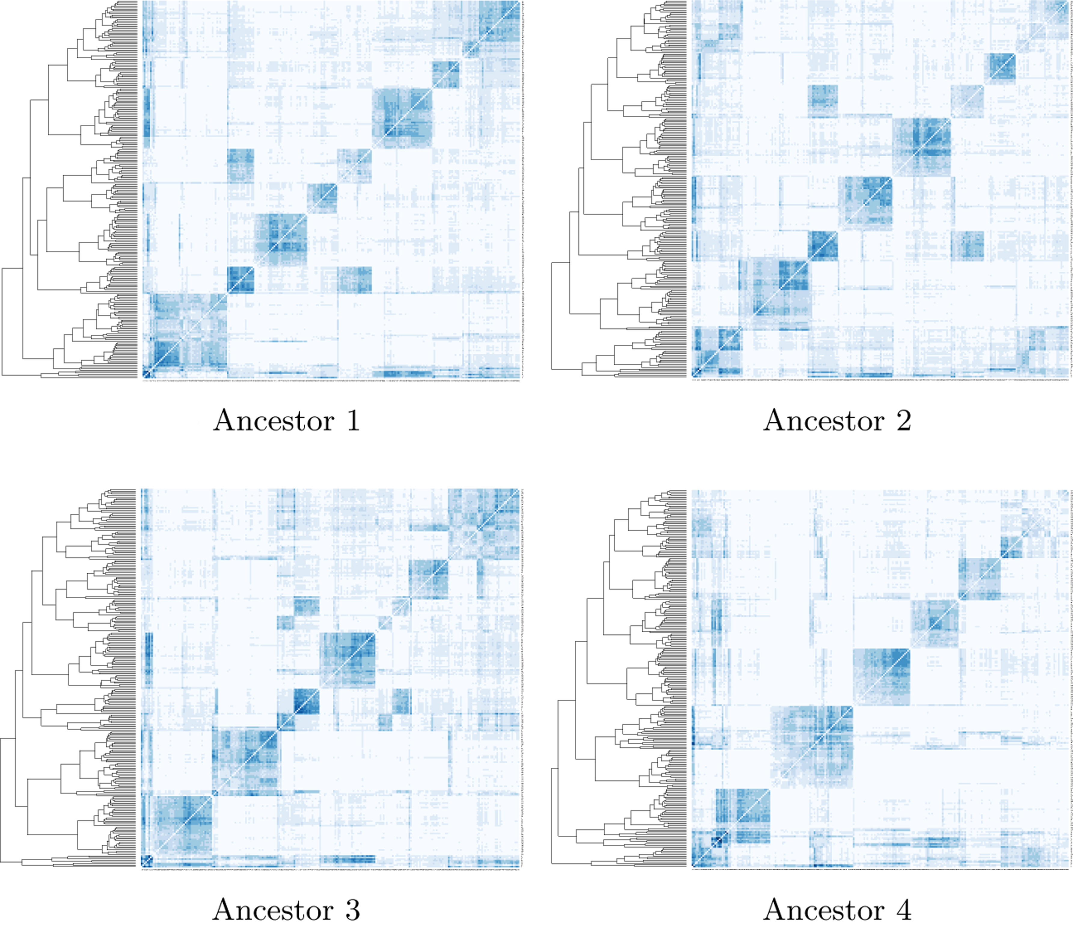
Heat maps of the four ancestors showing the clusters of contigs making up ancestral chromosomes from the longest 250 contigs by the complete-link clustering algorithm.

Table 5 contains statistics on the chromosomes and contigs.

Table 5.

Contigs and Genes in Ancestral Chromosomes

Chromosome	Ancestor 1		Ancestor 2		Ancestor 3		Ancestor 4
Chromosome	Contigs	Genes	Contigs	Genes	Contigs	Genes	Contigs	Genes
1	43	857	42	1398	40	1909	44	1911
2	40	729	43	585	43	683	46	703
3	23	363	21	443	22	467	18	620
4	44	951	39	671	42	853	38	917
5	41	773	43	894	32	656	40	810
6	23	536	23	666	30	958	31	985
7	36	743	39	844	41	497	33	411
Total	250	4952	250	5501	250	6013	250	6357

Although the four ancestral reconstructions in Figure 3 are very similar in their overall proportions of light and dark colors, in general we might want to enforce this comparability by ensuring that the proportions of pixels of each shade be fixed in advance. Table 6 gives the grayscales we settled on for this study.

Table 6.

The Fixed Proportion of Pixels with Its Corresponding Grayscale Intensity in Each Data Group Shown in the Heat Maps

Grayscale intensity	1	2	3	4	5	6	7	8	9
Proportion of pixels	50%	15%	10%	6%	4%	4%	4%	6.5%	0.5%

Figure 4 shows the improvement in visualizing the heat maps by using the co-occurrence correlations instead of the co-occurrence matrix.

FIG. 4.

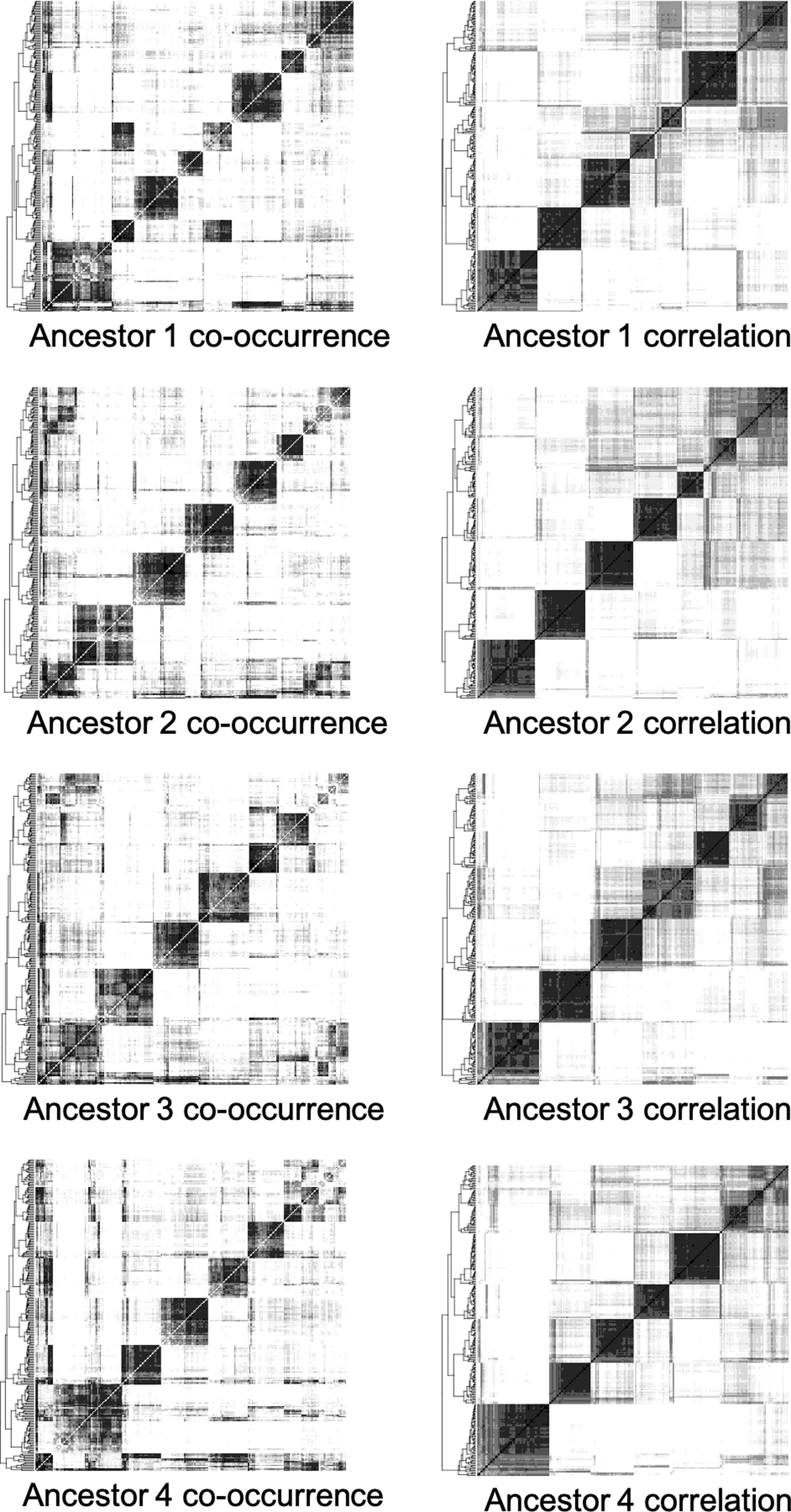
Heat maps of the four ancestors from the monocots data showing the clusters of contigs making up ancestral chromosomes from the longest 250 contigs, applying the complete-linkage clustering algorithm on chromosomal co-occurrence frequencies (left), and on correlations between co-occurrence vectors (right). The ordering of the contigs on the horizontal axis in each heat map is the same as that shown on the vertical axis.

3.3. Clustering corrections

The stepwise hierarchical procedure embodied in complete-link amalgamates two clusters I and J to form a larger cluster at each step, where I and J satisfy the min max criterion [minimum distance $d (i, j)$ between any elements $i \in I$ and $j \in J$ , over all clusters I and J existing at the time of the step]. The stepwise nature of this process means that the resulting hierarchy depends on input order of the elements. Often this means that a cluster that would usually form part of the output is fragmented into two or more parts. This is illustrated by the off-diagonal blocks in Figure 5. When such a configuration is evident, it is easily corrected by reordering the clusters involved, as indicated in the figure. This will result in a merger of the two clusters, with the removal of the off-diagonal blocks.

FIG. 5.

Correcting fragmented cluster.

Thus the first three blocks on the diagonal in the top left hand corner of Figure 3, together with two aligned off-diagonal blocks, could have been adjusted to produce two diagonal blocks.

3.4. Painting the chromosomes of the present-day genomes

Each chromosome in an ancestor genome is assigned a color. Despite the genome rearrangements intervening between an earlier ancestor and a later ancestor, corresponding chromosomes in different ancestral genomes can be identified by similarity in the gene content of their constituent contigs. This correspondence, though is disrupted in many places by interchromosomal exchanges, is reflected in the chromosomal color assignment in the four ancestors. The colors are then projected on to the chromosomes of the extant genomes that served as inputs to the pipeline, based on the contig matches detected in Section 3.1. Painting is carried out as described in Section 2.3 and is depicted in Figure 6.

FIG. 6.

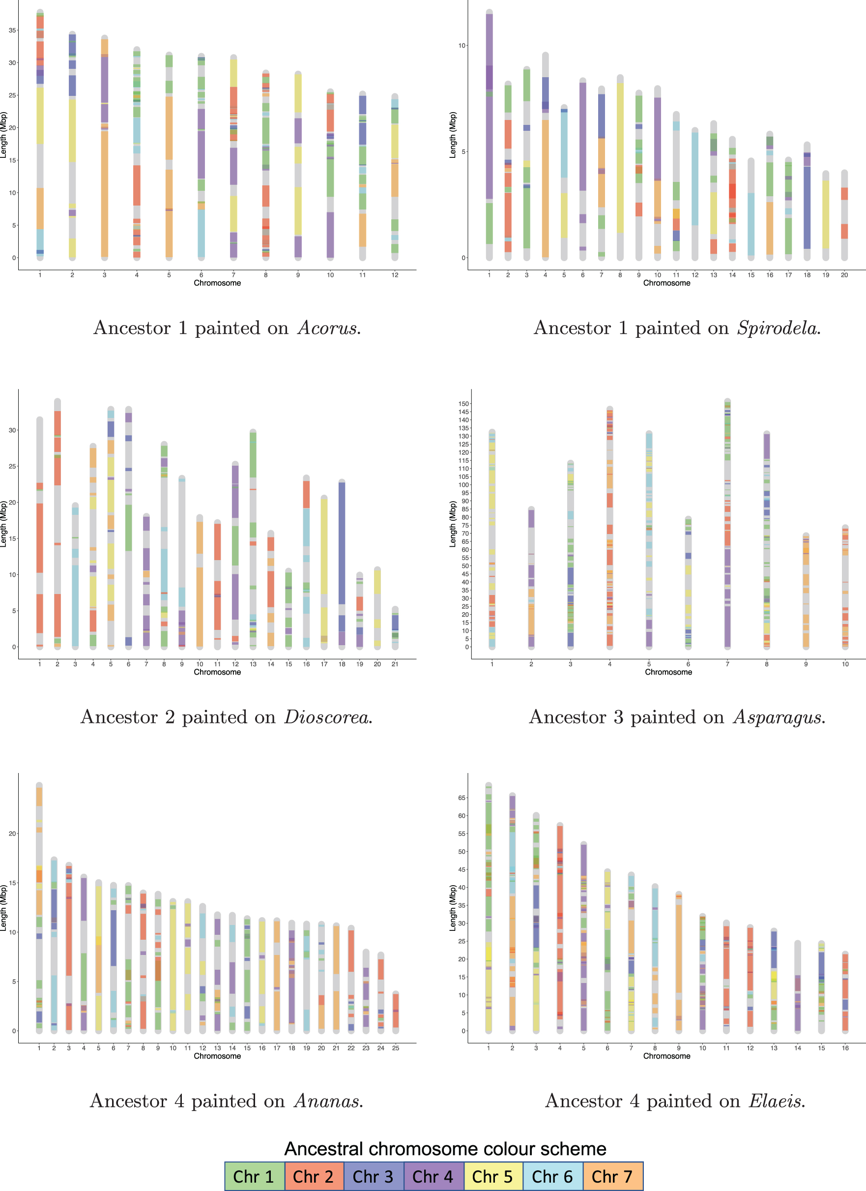
Chromosome painting of extant genomes according to the color assignment in their immediate ancestors. Ancestral blocks <150 Kbp are not shown.

3.5. Evaluation

Tables 7 and 8 provide quality assessments of the reconstruction as manifest in the painted extant genomes. In Table 7 we see a high degree of coverage of the extant genomes, whereas Table 8 gives a degree of choppiness that is moderate, given the time scale involved. Ancestors 1 and 2 achieve better coverage of all the extant genomes, even though most of the genomes were more directly involved in the reconstruction of Ancestors 3 and 4. This may be an artifact of the sparsity of matches from Ancestors 1 and 2, so that the interblock coloring discussed in Section 2.3 can cover longer uninterrupted regions of the chromosomes. A similar sparsity explanation can also be entertained for the low degree of choppiness of the paintings on the Spirodela genome, despite its higher degree of polyploidy than Acorus.

Table 7.

Percent Coverage of Extant Genomes by Ancestral Chromosomes

	Ancestor 1 (%)	Ancestor 2 (%)	Ancestor 3 (%)	Ancestor 4 (%)
Acorus	81	80	82	83
Spirodela	74	78	80	81
Dioscorea	54	61	62	63
Asparagus	63	62	66	71
Ananas	62	69	71	70
Elaeis	75	79	83	84

Table 8.

Choppiness of Painting on Extant Genomes

T	Acorus	Spirodela	Dioscorea	Asparagus	Ananas	Elaeis
Ancestor 1	45	33	48	40	48	59
Ancestor 2	38	22	45	38	38	57
Ancestor 3	48	36	48	43	42	60
Ancestor 4	50	39	57	47	55	65

$R - T$	Acorus	Spirodela	Dioscorea	Asparagus	Ananas	Elaeis
Ancestor 1	122	56	128	233	88	193
Ancestor 2	95	34	107	220	94	161
Ancestor 3	129	51	131	284	104	194
Ancestor 4	172	75	140	331	124	247

$R - X$	Acorus	Spirodela	Dioscorea	Asparagus	Ananas	Elaeis
Ancestor 1	134	63	136	239	106	216
Ancestor 2	112	45	121	221	100	196
Ancestor 3	142	64	143	283	110	215
Ancestor 4	170	74	166	337	137	270

T reflects how much interchromosomal exchange has occurred, $R - T$ is a measure of intrachromosomal movement (e.g., reversals or transpositions) and X is the number of small stripes <300 Kbp, which misleadingly inflates R.

3.6. MCScanX visualization

A different view of the evolution of the monocot genomes through ancestral intermediates is obtained through connecting homologous synteny blocks in a MCScanX visualization, as laid out in Figure 7. Consistent with the history of extensive rearrangement evident in Figure 6 and Table 8, the patterns of MCScanX connections are rather complex. Nevertheless, we can find important relationships using the “highlight” feature of the software.

FIG. 7.

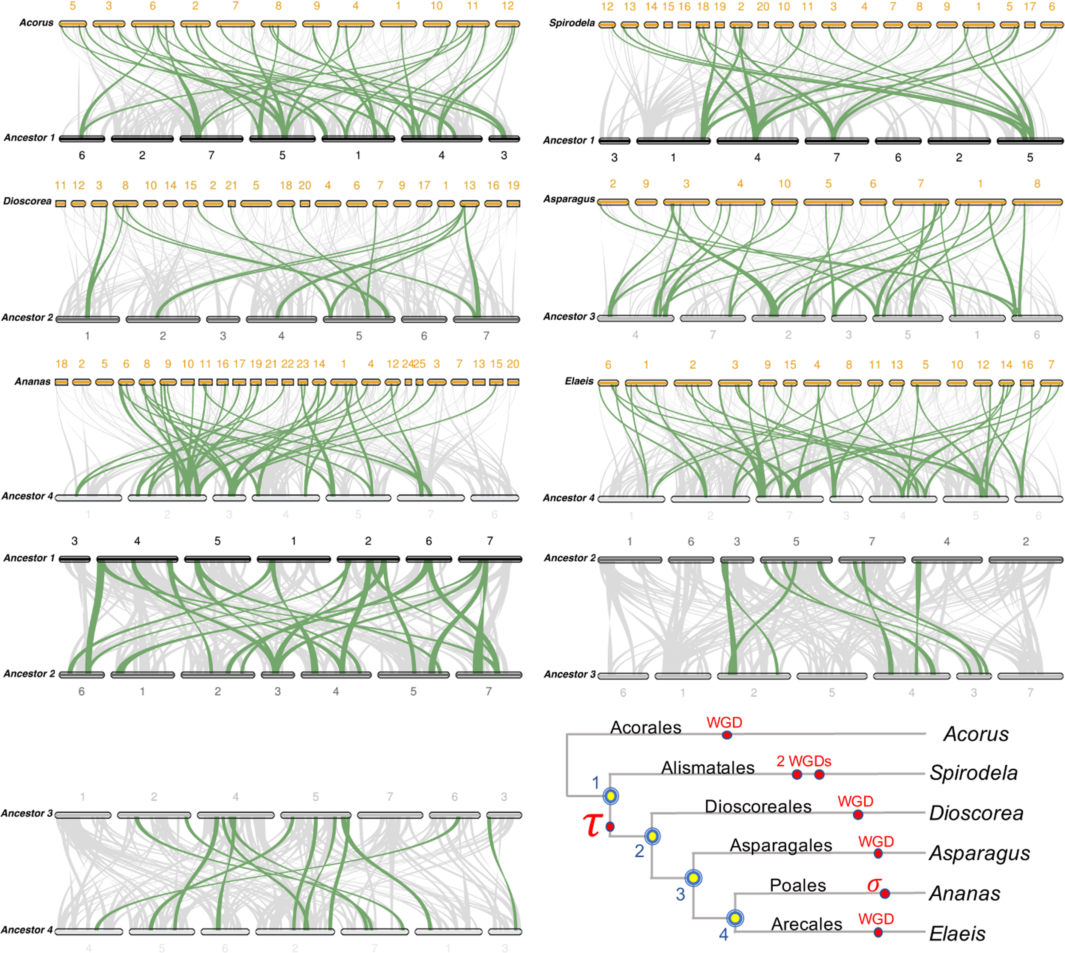
Matching genomes, extant and ancestral, with their immediate ancestors. WGD, whole genome duplication; WGT, whole genome triplication.

Thus, the comparison between Ancestor 1 and Acorus shows several chromosomal regions in the ancestor each linked to two regions in the extant genome, whereas the opposite pattern is nonexistent. Similarly the comparison between Ancestor 1 and Spirodela also shows instances of a 1:4 pattern, consistent with the two WGDs inherited by this species.

The most interesting pattern, however, is that between Ancestors 1 and 2, which strongly suggests a duplication event occurring before the branching of the Dioscorales from the main monocot stem lineage. In contrast, the Ancestor 2–Ancestor 3 and Ancestor 3–Ancestor 4 comparisons both show 1–1 patterns. Moreover, though dot-plot examination of Dioscorea evidences four subgenomes, thus two WGDs in its history, the MCScanX diagram of Ancestor 2-Dioscorea only shows evidence of one event, confirming that one event must have predated Ancestor 2. The latter event is the one shared by all the more recently branching orders, known as $τ$ .

3.7. How many chromosomes?

We note that the heat map for Ancestor 2 in Figure 3 differs little from that of Ancestor 1. There is no hint of a doubling of number of chromosomes. This can be understood in terms of the MWM construction where no gene family can appear more than once in the whole set of contigs. This militates against the recovery of two or more homologous chromosomes in the ancestor and in favor of a prepolyploidization version of the genome (Xu et al., 2021b).

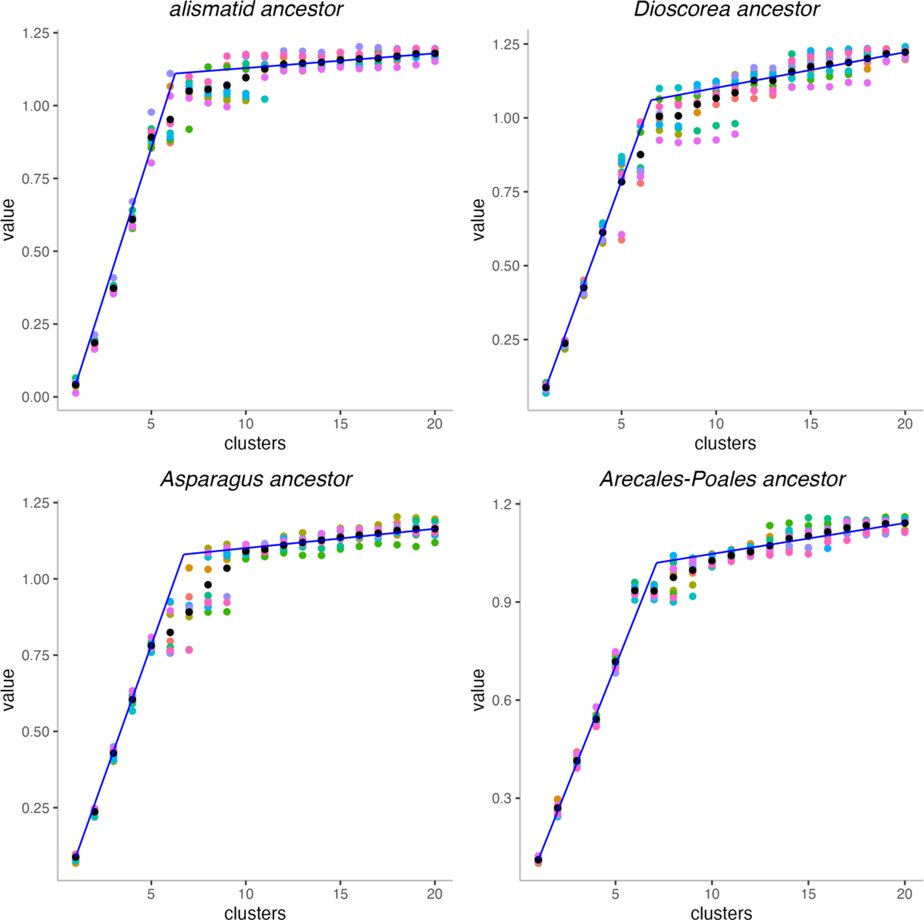
This understanding is reinforced by the gap statistics analysis depicted in Figure 8, based on 10 different MWM solutions. Here, a least squares fit of a line based on the gap values for $k = 1, \dots, 5$ , which measures the bonafide increase in cluster quality, intersects a line based on values for $k = 13, \dots, 20$ , where the small increases are due to overfitting. The cluster size k, where bonafide increases have been exhausted and overfitting is about to start, is close to 7 in all four ancestors. This confirms what the heat maps suggested, that the number of monoploids for the monocots is $x = 7$ , and is not affected by the $τ$ WGD.

FIG. 8.

Gap statistics analysis of monocot ancestors. Black dots are the means of 10 values for each k.

4. Reconstruction of the Solanaceae Ancestors

The RACCROCHE pipeline was developed using the monocot genomes for the test data set. It is important to know whether it will work on other data as well. On the basis of our familiarity with the Solanaceae (Zhang et al., 2018), we chose six species from this family: S. lycopersicum (tomato), S. tuberosum, S. melongena, C. annuum, N. tabacum (tobacco), and P. hybrida (petunia). These are phylogentically related as shown in Figure 9. The three Solanum species and Capsicum have 12 chromosomes, whereas the N. tabacum genome is a tetraploid with 24 chromosomes. P. hybrida has 14 chromosomes. Four ancestors, labeled with red circle at the divergent points of the tree in Figure 9, are reconstructed with the RACCROCHE. One known WGD between Ancestor 4 and tobacco is marked with a star on the branch.

FIG. 9.

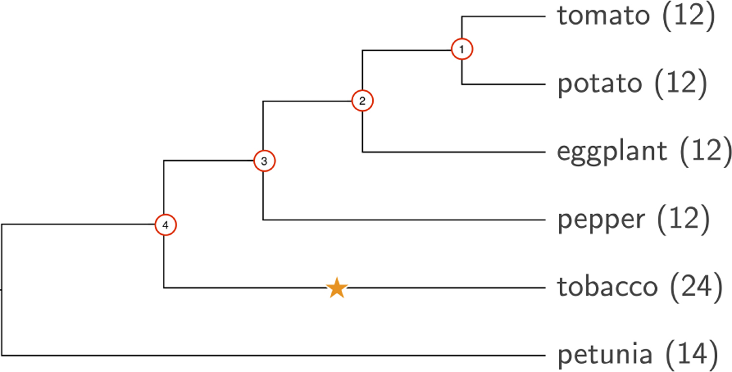
Phylogeny of Solanaceae. Root would be between Ancestor 4 and petunia.

The statistics of the reconstructed contigs for the four Solanaceae ancestors are listed in Table 9. The heat maps meant to depict the ancestral chromosomes of the four Solanaceae ancestors based on co-occurrence correlations appear in Figure 10.

FIG. 10.

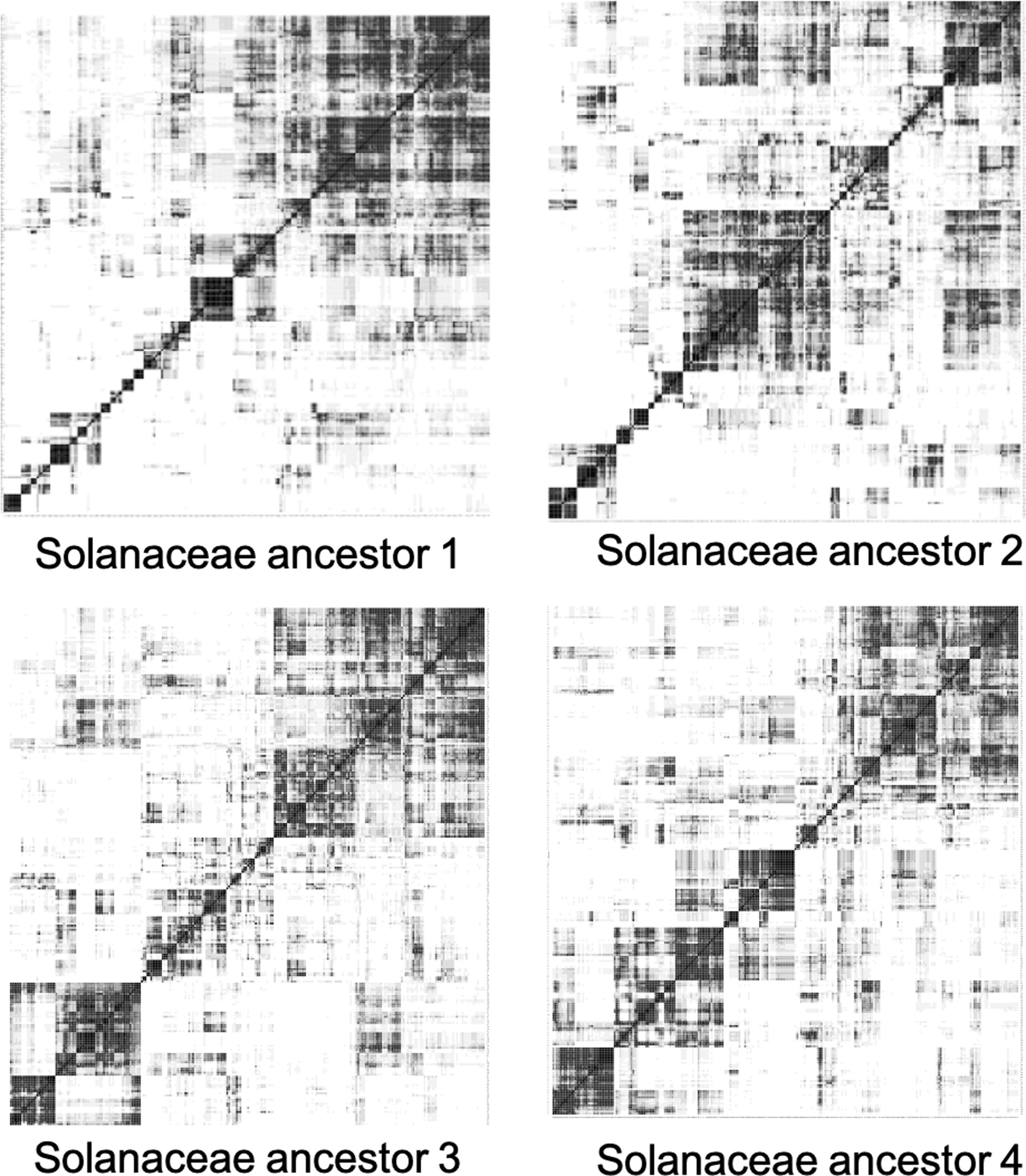
Heat maps of the four Solanaceae ancestors showing the clusters of contigs making up ancestral chromosomes from the longest 250 contigs by the complete-link clustering algorithm on co-occurrence correlation matrix.

Table 9.

Contig Statistics for the Four Solanaceae Ancestors

	Longest contig	Total number of contigs	N50
	Longest contig	Total number of contigs	Length	n
Ancestor 1	412	6313	80	67
Ancestor 2	270	14,058	7	289
Ancestor 3	175	15,426	1	757
Ancestor 4	151	16,883	1	756

The heat maps are a lot less clear than those of the monocots. The number of monoploids of the Solanaceae is said to be $x = 12$ (Särkinen et al., 2013; Bombarely et al., 2016), although Stevens (2001) allows the possibility that x = 6, stating “x = 12(?6,?11).” The heat maps for Ancestors 1 and 2, involving the tomato–potato–eggplant clade, show few clusters with many contigs, whereas Ancestors 3 and 4, weighted more toward the earlier branching tobacco, pepper, and petunia genomes, evidence five or six sizeable blocks. We turn to the gap statistics for the Solanaceae ancestors in Figure 11, to help interpret the heat map discordances. As with the monocots, the gap statistics are based on 10 different MWM solutions. The two least squares lines this time, however, are based on the gap values for $k = 1, \dots, 6$ , (bonafide increase in cluster quality), and on gap values for $k = 15, \dots, 20$ , (increases due to overfitting).

FIG. 11.

Gap statistics analysis of Solanaceae ancestors. Black dots are the means of 10 values for each k.

For Ancestors 1 and 2, the increase in gap values is relatively small, for all k. This reflects the relative absence of large clusters in the corresponding heat maps. Nevertheless there is a clear inflection point around $k = 12$ , corresponding to the conventionally accepted number of monoploids for Solanaceae, but also to the number of diploids for the four most closely related genomes in our study. In contrast, Ancestors 3 and 4 show a rapid rise in the gap statistic for small values of k, and an intersection of the two least squares lines around $k = 6$ . Again, this jibes with the heat maps for these ancestors, where about six ( $\pm 1$ ) clusters are clearly demarcated. This cannot be a reflection of the diverse haploid values of tobacco ( $n = 24$ ), petunia ( $n = 14$ ), and pepper ( $n = 12$ ). This confirms what the heat maps suggested, that the number of monoploids we calculated for the early branching species reflects an ancestral state existing before the so-called $x = 12$ clade within the Solanaceae originated. The gap statistics for the more recent ancestors may simply reflect commonalities among the highly rearranged genomes of the closely related tomato, potato, and eggplant species.

5. Evidence on Early Monoploid Status Internal to Each of Four Brassica Genomes

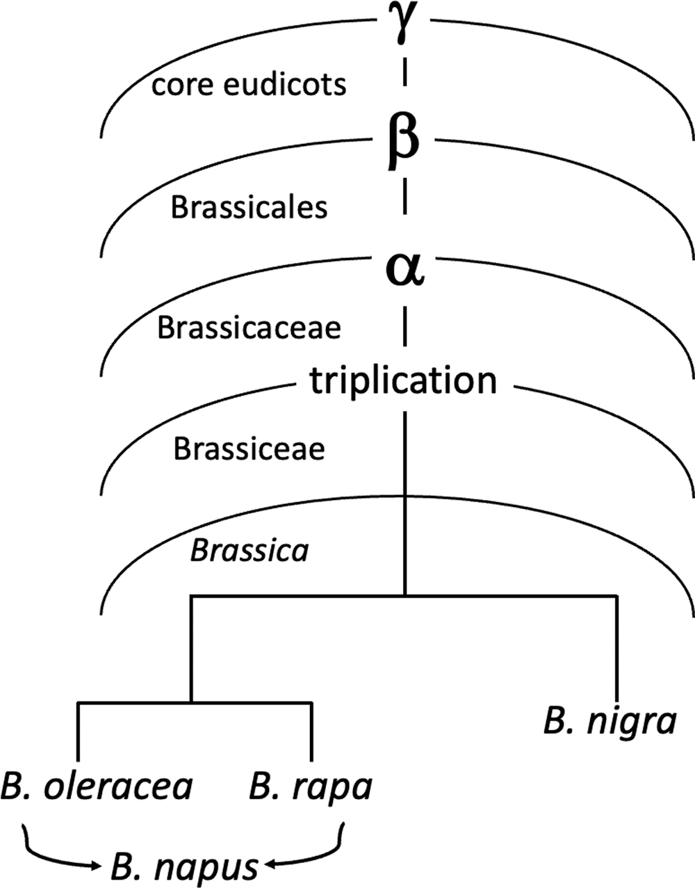
Of the six species in U's famous triangle (Kim et al., 2018), the three diploids, B. rapa (turnip, napa cabbage), B. oleracea (cabbage, cauliflower), and B. nigra (black mustard), as well as the allotetraploid B. napus (rapeseed, canola) formed from the first two, have all had their genomes sequenced (Perumal et al., 2020). These, and all species in the genus Brassica inherited the $γ$ WGT (Jaillon et al., 2007) giving rise to the core eudicots some 120 Mya, as well as the $β$ WGD during the evolution of the order Brassicales, ∼80 Mya, and the $α$ WGD within the family Brassicaceae (Barker et al., 2009; Edger et al., 2018) ∼23 Mya, as well as a more recent (5–9 Mya) triplication at the origin of the tribe Brassiceae (Lysak and Koch, 2011; Hao et al., 2021). This is schematized in Figure 12.

FIG. 12.

WGD or WGT history of Brassica genomes.

Thus the diploid Brassica species are descendants of at least four WGD or WGT events, the products of a $3 \times 2 \times 2 \times 3 = 36$ -fold replication of the original core eudicot progenitor, whereas the B. napus allotetraploid is the product of a 72-fold replication of this progenitor.

In the previous sections, we addressed the problem of extracting the underlying or ancestral monoploid genome from its diverse transformations—duplicated, rearranged, etc.—represented by a number of present-day genomes and subgenomes in a phylogenetic tree subtended by that ancestor. Given the extensive history of genome replication in the evolution of Brassica, we can ask to what extent repetitive features of ancestral chromosomal structure persist in each of the modern genomes analyzed separately.

The Brassiceae triplication is thought to have increased the number of chromosomes from 7 to 21, but that was subsequently reduced to 8 or 9 before the series of speciations, which gave rise to the U's triangle species. The reconstructed ancestor of B. nigra, B. oleracea, and B. rapa has 9 chromosomes (Perumal et al., 2020), whereas the modern genomes have 8, 9, and 10 chromosomes, respectively. B. napus has 19 chromosomes.

Figure 13 shows the result of applying RACCROCHE to the genomes of each of the Brassica spp. individually—omitting the cross-species construction of gene families as well as the phylogenetic filtering step. These heat maps, although not as clear as those we observed for the monocots, are much clearer than those from Solanaceae. The quality of the Brassica contigs is given in Table 10.

FIG. 13.

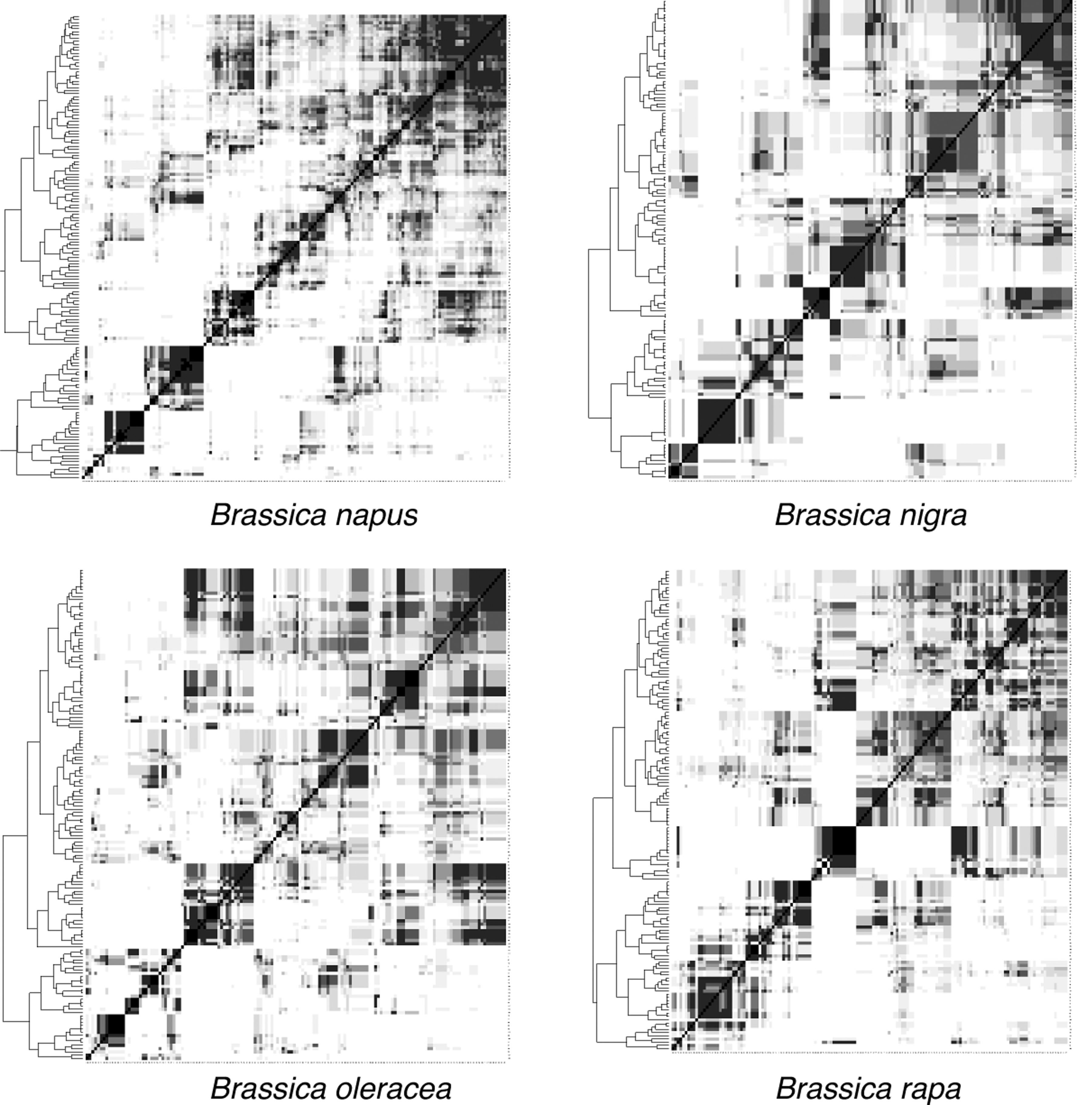
Heat map of the reconstructed Brassica ancestors.

Table 10.

Contig Statistics for Brassica nigra, Brassica oleracea, Brassica rapa, and Brassica napus Ancestors

Ancestor of	Longest contig	Total number of contigs	N50		N60		N70
Ancestor of	Longest contig	Total number of contigs	Length	n	Length	n	Length	n
B. nigra	250	428	80	35	67	48	46	65
B. oleracea	151	816	49	55	39	80	28	106
B. rapa	209	524	54	46	44	63	35	84
B. napus	383	550	117	41	89	55	68	73

The displays for all the diploid genomes suggest eight or fewer chromosomes. The heat map for B. napus clearly shows far fewer than its current complement of 19 chromosomes, perhaps 12, more in keeping with the chromosome counts of its two progenitors B. rapa (10 chromosomes) and B. oleraceae (9 chromosomes).

The gap statistics shown in Figure 14 largely confirm the impression that the ancestral Brassica genome had fewer chromosomes than its descendants, with inflection points at k = 5, 6, and 8. And the allotetraploid B. napus shows an inflection at 12, which is not as low as its progenitors, but much lower than its current complement of 19 chromosomes.

FIG. 14.

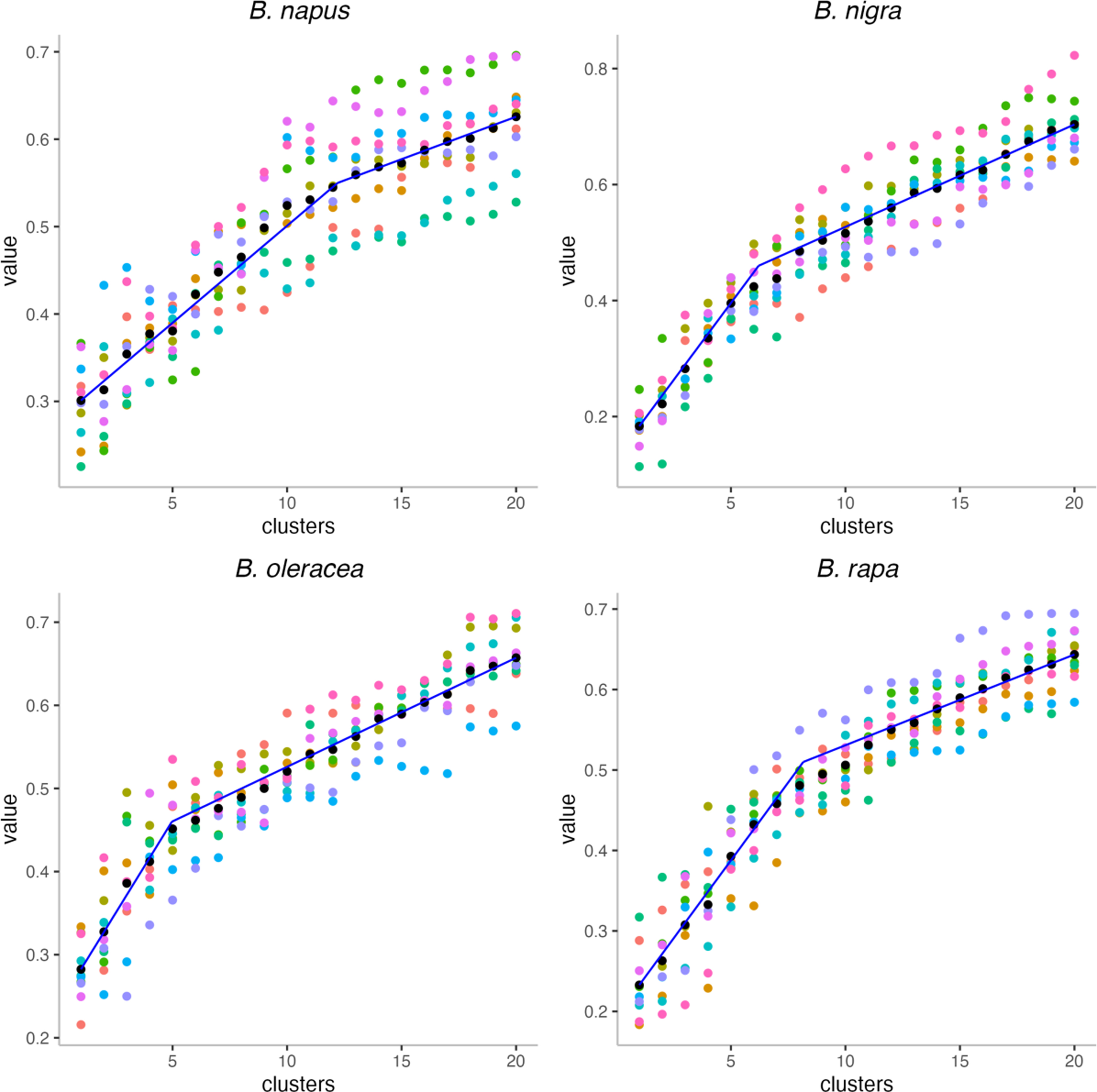
Gap statistics analysis within the reconstructed Brassica ancestors. Black dots are the means of 10 values for each k.

That RACCROCHE is reconstructing an earlier stage of evolution, namely the ancestor of its two progenitors. The reconstruction is consistent with the suggestion in Xu et al. (2021b) that this method detects ancestral monoploids, rather than more recent polyploid stages in the ancestor.

6. Discussion and Conclusions

This study explores an alternative approach to existing methods for ancestral genome reconstruction. Rather than identifying shared adjacencies between pairs of putatively orthologous anchor genes, we compile a large number of potential components and use a combinatorial optimization approach to combining them, an approach explicitly disavowed by, for example, Perrin et al. (2015). We were motivated by the special challenges in plant comparative genomics posed by recurrent polyploidization and fractionation. Compared with approaches such as proCARs (Perrin et al., 2015) that is very successful in reconstructing ancestral animal genomes, RACCROCHE may work better with plant genomes, since it is designed to be robust to the gene order scrambling effect of polyploidy and fractionation.

Since the entities reconstructed by proCARs are not meant to be individual ancestral genes, but blocks of syntenically related genes identified at the level of extant genomes, it is hard to compare our inferred ancestral genomes, composed of hypothetical genes with identifiable functions, with the output of proCARs. In our hands proCARs identified 214 synteny blocks in our monocot data, organized into “CARs” making up the ancestral genomes. These contained a total of 3248 “universal seeds,” which may be comparable with our ancestral genes, although our ancestors contained about twice as many. Insofar as these comparisons are valid, they confirm the utility of RACCROCHE in plant comparative genomics.

One particular feature that stands out in this study is the innovative clustering of counts of contig co-occurrences on extant chromosomes, or of the correlation of these co-occurrences, followed by heat map construction to identify ancestral chromosomes. Although it required very little manual effort to identify the monocot clusters in Figure 3 or Figure 4, the situation with Solanaceae in Figure 10 and Brassica genomes in Figure 13 is less clear. To deal with this, we introduced gap statistics to detect the point of diminishing returns when postulating successively larger values for the number of chromosomes. Future study will include an investigation of block modeling theory (Lee and Wilkinson, 2019) to develop a clustering procedure that is both objective and visually compelling.

Another innovation is the use of MCScanX to assess the consequences of WGDs for the evolution of chromosomal gene content and order along internal branches of a species phylogeny.

As a consequence of the MWM step in our pipeline, the whole set of output contigs can contain each gene family at most once. This precludes the appearance of homologous chromosomes and this tends to reconstruct prepolyploidization versions of ancestral genomes. This is seen most clearly in the lilioid Ancestors 2, 3, and 4 of the monocot construction, and in the reconstruction of the ancestor of B. napus. Taking advantage of this feature may allow us to reconstruct the hypothetical monoploid at the origin of a family or order (Xu et al., 2021b).

Our use of gap statistics involves taking a mean over a sample of MWM outputs. This leads to two problems. First is the heavy computing requirements. The second is the considerable scatter of the gap statistic for a given k, so that we cannot put too much credence in any one data point. This includes any particular heat map. In contrast, the use of gap statistics offers a new opening to the statistical evaluation of reconstruction.

Footnotes

Acknowledgments

We thank the Department of Energy Joint Genome Institute staff and collaborators including David Kudrna, Jerry Jenkins, Jane Grimwood, Shengqiang Shu, and Jeremy Schmutz for prepublication access to the Acorus genome sequence and annotation. Thanks to Aîda Ouangraoua for much help in implementing ProCARs (Perrin et al., 2015) and Haibao Tang for responding to queries about MCScanX (Wang et al., ).

Availability

The annotated genomic data are accessible on the CoGe platform https://genomevolution.org/coge/and Phytozome. The pipeline is available at .

Author Disclosure Statement

The authors declare they have no competing financial interests.

Funding Information

Research supported by Discovery grants to L.J. and D.S. from the Natural Sciences and Engineering Research Council of Canada. D.S. holds the Canada Research Chair in Mathematical Genomics.

References

Amborella Genome Project. 2013. The Amborella genome and the evolution of flowering plants. Science, 342, 1241089.

Anselmetti

, Luhmann

, Bérard

, et al. 2018. Comparative methods for reconstructing ancient genome organization, 343–362. In Setubal, J., Stoye, J., and Stadler, P., eds. Comparative Genomics. Springer, New York.

Avdeyev

, Alexeev

, Rong

, et al. 2020. A unified ILP framework for core ancestral genome reconstruction problems. Bioinformatics, 36, 2993–3003.

Badouin

, Gouzy

, Grassa

C.J.

, et al. 2017. The sunflower genome provides insights into oil metabolism, flowering and asterid evolution. Nature, 546, 148–152.

Barker

M.S.

, Vogel

, and Schranz

M.E.

2009. Paleopolyploidy in the brassicales: Analyses of the cleome transcriptome elucidate the history of genome duplications in arabidopsis and other brassicales. Genome Biol Evol, 1, 391–399.

Bombarely

, Moser

, and Amrad

2016. Insight into the evolution of the solanaceae from the parental genomes of Petunia hybrida. Nat. Plants, 2, 16074.

Chauve

, and Tannier

2008. A methodological framework for the reconstruction of contiguous regions of ancestral genomes and its application to mammalian genomes. PLoS Comput. Biol. 4, e1000234.

Edger

P.P.

, Hall

J.C.

, Harkess

, et al. 2018. Brassicales phylogeny inferred from 72 plastid genes: A reanalysis of the phylogenetic localization of two paleopolyploid events and origin of novel chemical defenses. Am. J. Bot. 105, 463–469.

Gagnon

, Blanchette

, and El-Mabrouk

2012. A flexible ancestral genome reconstruction method based on gapped adjacencies. BMC Bioinformatics 13 (Suppl. 19), S4.

10.

Givnish

T.J.

, Zuluaga

, Spalink

, et al. 2018. Monocot plastid phylogenomics, timeline, net rates of species diversification, the power of multi-gene analyses, and a functional model for the origin of monocots. Am. J. Bot. 105, 1888–1910.

11.

Hao

, Mabry

M.E.

, Edger

P.P.

, et al. 2021. The contributions from the progenitor genomes of the mesopolyploid Brassiceae are evolutionarily distinct but functionally compatible. Gen. Res. 31, 799–810.

12.

Jaillon

, Aury

J.-M.

, Noel

, et al. 2007. The grapevine genome sequence suggests ancestral hexaploidization in major angiosperm phyla. Nature, 449, 463.

13.

Kim

C.K.

, Seol

Y.J.

, Perumal

, et al. 2018. Re-exploration of U's triangle Brassica species based on chloroplast genomes and 45S nrDNA sequences. Sci. Rep., 8, 7353.

14.

Lee

, and Wilkinson

D.J.

2019. A review of stochastic block models and extensions for graph clustering. Appl. Netw. Sci. 4, 122.

15.

Lysak

M.A.

, and Koch

M.A.

2011. Phylogeny, genome, and karyotype evolution of crucifers (Brassicaceae), 1–31. In Schmidt, R., and Bancroft, I., eds. Genetics and Genomics of the Brassicaceae. Springer, New York.

16.

, Zhang

, Suh

B.-B.

, et al. 2006. Reconstructing contiguous regions of an ancestral genome. Gen. Res. 16, 1557–1565.

17.

Martí

, Reinelt

, and Duarte

2012. A benchmark library and a comparison of heuristic methods for the linear ordering problem. Comput. Optim. Appl. 51, 1297–1317.

18.

Mayrose

, and Lysak

M.A.

2021. The evolution of chromosome numbers: Mechanistic models and experimental approaches. Gen. Biol. Evol. 13, evaa220.

19.

Mazowita

, Haque

, and Sankoff

2006. Stability of rearrangement measures in the comparison of genome sequences. J. Comput. Biol. 13, 554–566.

20.

Murat

, Armero

, Pont

, et al. 2017. Reconstructing the genome of the most recent common ancestor of flowering plants. Nat. Genet. 49, 490–496.

21.

Perrin

, Varré

J.-S.

, Blanquart

, et al. 2015. ProCARs: Progressive reconstruction of ancestral gene orders. BMC Genomics, 16(S5), S6.

22.

Perumal

, Koh

C.S.

, Jin

, et al. 2020. A high-contiguity Brassica nigra genome localizes active centromeres and defines the ancestral Brassica genome. Nat. Plants, 6, 929–941.

23.

Qin

, Hu

Y. W

, ang

, et al. 2021. Insights into angiosperm evolution, floral development and chemical biosynthesis from the Aristolochia fimbriata genome. Nat. Plants, 7, 1239–1253.

24.

Rubert

D.P.

, Martinez

F.V.

, Stoye

, et al. 2020. Analysis of local genome rearrangement improves resolution of ancestral genomic maps in plants. BMC Genomics, 21, 1–11.

25.

Särkinen

, Bohs

, Olmstead

R.J.

, et al. 2013. A phylogenetic framework for evolutionary study of the nightshades (Solanaceae): A dated 1000-tip tree. BMC Evol. Biol. 13, 214.

26.

Schiavinotto

, and Stützle

2004. The linear ordering problem: Instances, search space analysis and algorithms. J. Math. Modell. Algorithms, 3, 67–402.

27.

Stevens

P.F.

2001. Solanaceae. (Entry in Angiosperm Phylogeny Website. Version 14). Available at: www.mobot.org/MOBOT/research/APweb/. Accessed August 2021 .

28.

Tannier

, Bazin

, Davín

, et al. 2020. Ancestral genome organization as a diagnosis tool for phylogenomics, 2.5:1–2.5:19. In Scornavacca, C., Delsuc, F., and Galtier, N., eds. Phylogenetics in the Genomic Era. No Commercial Publisher; Authors Open Access Book.

29.

Tibshirani

, Walther

, and Hastie

2001. Estimating the number of clusters in a data set via the gap statistic. J. R. Stat. Soc. Ser. B (Stat. Methodol.), 63, 411–423.

30.

Wang

, Tang

, DeBarry

J.D.

, et al. 2012. MCScanX: A toolkit for detection and evolutionary analysis of gene synteny and collinearity. Nucleic Acids Res. 40, e49.

31.

, Jin

, Leebens-Mack

J.H.

, et al. 2021c. Validation of automated chromosome recovery in the reconstruction of ancestral gene order. Algorithms 14, 160.

32.

, Jin

, Zheng

, et al. 2021a. RACCROCHE: Ancestral flowering plant chromosomes and gene orders based on generalized adjacencies and chromosomal gene co-occurrences. Lect. Notes Bioinform. 12686, 97–115.

33.

, Zhang

, et al. 2021b. The monoploid chromosome complement of reconstructed ancestral genomes in a phylogeny. RECOMB CG 2021, 1–12.

34.

, and Sankoff

2008. Tests for gene clusters satisfying the generalized adjacency criterion, 152–160. In Bazzan, A.L.C., Craven, M., and Martins, N.F., eds. Brazilian Symposium on Bioinformatics. Springer, New York.

35.

Yang

, and Sankoff

2010. Natural parameter values for generalized gene adjacency. J Comput Biol, 17, 1113–1128.

36.

Zhang

, Zheng

, and Sankoff

2018. Speciation and rate variation in a birth-and-death account of WGD and fractionation; the case of Solanaceae, 146–160. In Blanchette, M., and Ouangraoua, A., eds. Comparative Genomics. Springer, New York.

37.

Zhao

, Zwaenepoel

, Xue

J.-Y.

, et al. 2021. Whole-genome microsynteny-based phylogeny of angiosperms. Nat. Commun. 12, 3498.

38.

Zheng

, Chen

, Albert

V.A.

, et al. 2013. Ancient eudicot hexaploidy meets ancestral eurosid gene order. BMC Genomics, 14(S7), S3.

Ancestral Flowering Plant Chromosomes and Gene Orders Based on Generalized Adjacencies and Chromosomal Gene Co-Occurrences

Abstract

1. Introduction

2. Methods

2.1. Input

2.2. The pipeline

2.2.1. Step 1: Preprocess gene families

2.2.2. Step 2: List generalized adjacencies

2.2.3. Step 3: List candidate adjacencies

2.2.4. Step 4: Construct contigs

2.2.5. Step 5: Match synteny blocks between ancestral genome and extant genomes

2.2.6. Step 6: Cluster ancestral contigs into ancestral chromosomes

2.2.7. Step 6a: Use of gap statistics to estimate the number of chromosomes when it is not clear from the heat map

2.3. Visualizing and evaluating the reconstruction

2.3.1. Step 7: Painting the extant genomes according to the ancestral chromosomes

2.3.2. Step 8: Adapting MCScanX to match ancestral genomes with extant genomes

2.3.3. Step 9: Measures of quality

3. Reconstruction of Monocot Ancestors

3.1. Properties of the contig reconstruction

3.2. Clustering

3.3. Clustering corrections

3.4. Painting the chromosomes of the present-day genomes

3.5. Evaluation

3.6. MCScanX visualization

3.7. How many chromosomes?

4. Reconstruction of the Solanaceae Ancestors

5. Evidence on Early Monoploid Status Internal to Each of Four Brassica Genomes

6. Discussion and Conclusions

Footnotes

Acknowledgments

Availability

Author Disclosure Statement

Funding Information

References