Sage Journals: Discover world-class research

Abstract

Methods for translating gene expression signatures into clinically relevant information have typically relied upon having many samples from patients with similar molecular phenotypes. Here, we address the question of what can be done when it is relatively easy to obtain healthy patient samples, but when abnormalities corresponding to disease states may be rare and one-of-a-kind. The associated computational challenge, anomaly detection, is a well-studied machine-learning problem. However, due to the dimensionality and variability of expression data, existing methods based on feature space analysis or individual anomalously expressed genes are insufficient. We present a novel approach, CSAX, that identifies pathways in an individual sample in which the normal expression relationships are disrupted. To evaluate our approach, we have compiled and released a compendium of public expression data sets, reformulated to create a test bed for anomaly detection. We demonstrate the accuracy of CSAX on the data sets in our compendium, compare it to other leading methods, and show that CSAX aids in both identifying anomalies and explaining their underlying biology. We describe an approach to characterizing the difficulty of specific expression anomaly detection tasks. We then illustrate CSAX's value in two developmental case studies. Confirming prior hypotheses, CSAX highlights disruption of platelet activation pathways in a neonate with retinopathy of prematurity and identifies, for the first time, dysregulated oxidative stress response in second trimester amniotic fluid of fetuses with obese mothers. Our approach provides an important step toward identification of individual disease patterns in the era of precision medicine.

1. Introduction

The development in the 1990s of techniques for genome-wide monitoring of expression data (Lockhart et al., 1996; Shalon et al., 1996) has had a dramatic impact on the field of molecular medicine. Precision diagnostics based on expression array signatures are increasingly moving into the clinic (Mehta et al., 2011; Glas et al., 2006). However, methods for designing microarray-based diagnostics or discovering disease subtypes require a reasonable number of samples representing each patient class (Slonim, 2002). There are techniques for boosting the signal when relatively few samples are available (Tusher et al., 2001; Dougherty, 2001), but these don't eliminate the need for a representative set of samples that fully characterize the molecular variability underlying the phenotypes of interest. For rare diseases or genetically heterogeneous disorders, another analysis paradigm is needed. Here we demonstrate that by characterizing the expression patterns of “normal” samples, it is often possible to identify abnormal samples even when each abnormality is one-of-a-kind.

The problem of determining which samples to flag as abnormal, given only normal training data, is related to the computational field of anomaly detection, sometimes called outlier detection. Anomaly detection is an active research area in both statistics and data mining (Chandola et al., 2009). It is regularly applied to such problems as spam detection, identifying potential credit-card theft, verifying online identities, and correcting errors in census data.

Several previous efforts explicitly apply anomaly detection to bioinformatics problems, including correction in genome annotation (Mikkelsen et al., 2005) and identifying changes in the steady-state behavior of stochastic gene regulatory networks (Kim and Gelenbe, 2009). A related approach by Torkamani and Schork (2009) identifies genes whose expression pattern is unusual in a given cellular context. For gene expression microarray data, the task of identifying differentially expressed genes has been viewed in the framework of outlier detection (Mpindi et al., 2011; Li et al., 2007; Ghosh, 2010; Karrila et al., 2011), as has the problem of identifying array artifacts (Sauer et al., 2005). Perhaps the closest approach to ours is that of Tomlins et al. (2005), who use outlier detection to identify common translocations in cancer, but the outliers still refer to individual genes rather than samples.

The underlying machine learning problem, that of identifying “abnormal” samples given only “normal” samples as training data, is a challenging one. Microarray data is particularly ill-suited for anomaly detection, as for many other machine learning problems, because of its noise level, the dimensionality of a typical data set (hundreds of samples but tens of thousands of genes), and the expectation that only a small fraction of those genes may provide any information about the classification of the samples.

Fortunately, other characteristics make the problem potentially tractable. We expect meaningful expression changes to reflect unusual regulation in specific functional pathways. We can therefore use prior knowledge about the relationships between genes to identify anomalous examples. Such information has the added advantage that it may provide hints to the underlying cause of the detected anomalies.

To evaluate the utility of such an approach, we created a compendium of data sets for anomaly detection from published microarray classification data sets. On this compendium, we compare several state-of-the-art methods for anomaly detection, including CSAX, a novel approach that we designed to boost the signal from the prior method most robust to irrelevant features (Noto et al., 2011) while identifying the gene sets that best distinguish each anomalous sample. Our results show that in many cases, anomaly detection can both identify unusual samples and produce meaningful information about the nature of the anomalous data.

There is also a question of what abnormalities we can expect to identify. For example, a single abnormal sample characterized by abnormal expression of a single gene could not possibly be detected by any method—the data are simply too noisy. Our method is applicable when a sizable number of genes' expression levels are sufficiently different. We characterize the classes of anomalies we can expect to detect, and we discuss how clinical intuition might be applied to identify anomalies suitable for these methods. Our inspiration for this work came from prenatal and neonatal genomics, where recognizing and interpreting rare developmental abnormalities is crucial. We therefore conclude with a case study illustrating how our methods can contribute in this setting.

2. Data and Methods

2.1. Compendium of microarray anomaly detection data sets

We assembled a compendium of 28 anomaly detection tasks from published gene expression classification studies that involve at least two classes of samples (e.g., healthy vs. disease). We convert these to anomaly detection tasks by (i) designating one class as the “anomalous” class, and all samples from the other classes as the “normal” class, which may therefore be quite heterogeneous; (ii) creating a training set from a random subset of normal microarrays; and (iii) creating a test set from the remaining samples (Fig. 1). We created our compendium from suitably sized data sets with at least two clearly defined classes found in GEO, combined with a testbed of expression classification data sets assembled elsewhere for the development of computational methods (see Acknowledgments section). The compendium includes all the data sets with which we experimented that had previouly been released publicly (Supplementary Material, available online at www.liebertonline.com/cmb).

FIG. 1.

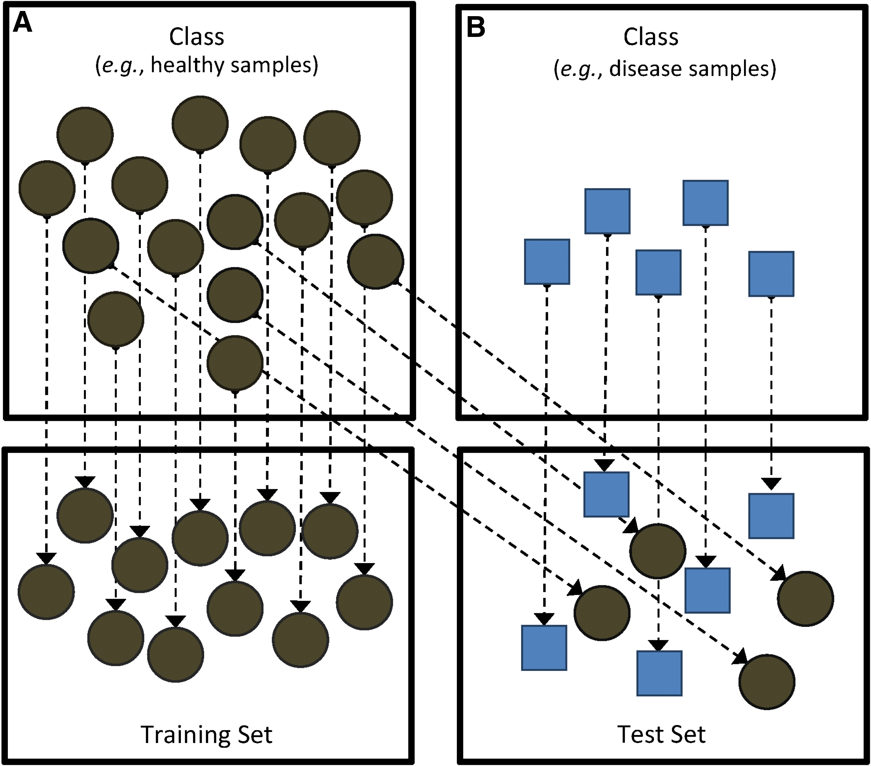
To create an anomaly detection task from a microarray study with two classes of samples, A and B, we randomly select a portion of the A samples for the test set and use the remainder for training. The task is then to identify samples from class B after training on samples from class A alone.

In most envisioned applications, such as diagnosing rare developmental disorders, abnormalities are likely to be one of a kind. However, in each data set in this compendium, we have a collection of relatively similar anomalies, and we know which samples we should expect to identify as anomalous. We therefore use this compendium as a “gold standard” data set to evaluate the accuracy of our methods.

2.2. Methods for expression anomaly detection

2.2.1. Prior methods

There are many existing methods for anomaly detection in high-dimensional data. The most successful general approaches include density-based methods such as the local outlier factor (LOF) (Breunig et al., 2000), which identifies outliers by comparing their distances from their nearest neighbors to the typical distances between nearby training examples, and one-class support vector machines (SVMs) (Schölkopf et al., 2000). To compare the approaches described below to one-class support vector machines (Schölkopf et al., 2000), we use the LIBSVM (Chang and Lin, 2001) implementation with default settings. Preliminary investigation showed that results were not sensitive to a wide range of parameter settings (data not shown).

To compare our approach to LOF (Breunig et al., 2000), we use our own implementation. LOF requires the specification of a single parameter, MinPts, which is the size of the neighborhood of microarrays. Following a suggestion in the original presentation of LOF (Breunig et al., 2000), we compute the LOF using all possible values of MinPts and take the maximum LOF. Source code and documentation for our implementation can be found in the Supplementary Material.

However, neither of these prior methods is especially well suited for handling the dimensions of expression microarray data. We recently developed an anomaly-detection method called feature regression and classification, or FRaC (Noto et al., 2010, 2011). FRaC learns relationships among gene expression in the training data and measures their reliability. It uses those models to estimate the likelihood of test set expression. The extent to which a test set gene's expression is considered anomalous is measured by the log-loss of its likelihood, according to those models. Anomaly scores for samples are computed by summing anomaly scores over all genes. FRaC is known to be robust to large numbers of irrelevant variables (Noto et al., 2011), making it well suited for identifying outliers in expression data.

Because FRaC forms the core of our new method below, we give a brief summary here. Given a training set and an unlabeled test example, FRaC does the following for all genes i:

1. Infer a predictive model C_i of the expression of gene i from the training data. The model will use the expression of some of the other genes to make its predictions. For this step, we use an ε-SVR (support vector regression) model with a linear kernel, the ε parameter (in the loss function) set to zero, and the C parameter (for regularization) set to 1. Preliminary experiments with expression anomaly detection showed that FRaC is not very sensitive to these choices, and these settings prove to work well (data not shown).

2. Use held-aside training data (i.e., not used in the previous step) to estimate the accuracy of the model by building a model E_i of the predictive error. We use leave-one-out cross-validation to sample the predictive error, and we model E_i as a normal distribution \documentclass{aastex}\usepackage{amsbsy}\usepackage{amsfonts}\usepackage{amssymb}\usepackage{bm}\usepackage{mathrsfs}\usepackage{pifont}\usepackage{stmaryrd}\usepackage{textcomp}\usepackage{portland, xspace}\usepackage{amsmath, amsxtra}\pagestyle{empty}\DeclareMathSizes{10}{9}{7}{6}\begin{document} $${ \cal N} ( \mu , \sigma )$$ \end{document} , where μ and σ are set to the sample mean and standard deviation, respectively.

3. Use the predictive model C_i to predict the expression of gene i in the unlabeled example.

4. Compute the likelihood of the error of the prediction using the error model E_i.

5. The anomaly score we assign to gene i is the log loss, or surprisal, of the likelihood computed in the previous step.

The anomaly score for the test sample is computed as the sum of the anomaly scores for each gene. We use our own implementation of FRaC; the source code and documentation are available in the Supplementary Material.

2.2.2. CSAX: A new method for expression anomaly detection

All of the above methods classify samples as outliers, but do not explicitly provide information about the nature of each anomaly. Instead, our goal is to identify gene sets or pathways in which a sample is particularly anomalous. We therefore developed a robust method, Characterizing Systematic Anomalies in eXpression data (CSAX), for doing so, taking advantage of FRaC's robustness to irrelevant variables.

CSAX uses FRaC to compute an anomaly score for each gene and uses Gene Set Enrichment Analysis (GSEA) (Subramanian et al., 2005; Mootha et al., 2003) to find gene sets containing many genes whose expressions are particularly surprising. GSEA is implemented in Java and available Online. We use the Java archive (gsea2-2.07.jar) and run the “preranked” version of GSEA (xtools.gsea.GseaPreranked) on gene sets with at least 7 and at most 500 genes, with 1000 permutations and a weighted scoring scheme (see GSEA documentation). GSEA in this case takes as input a list of genes, ranked by their anomaly scores, and a collection of gene sets. The output of GSEA is a table, listing each gene set, its enrichment score (see Subramanian et al., 2005; Mootha et al., 2003, for details), and other statistics, including a normalized version of the enrichment score that accounts for gene set size.

This approach alone, which we call FRaC + enrichment, has the important advantage of identifying the gene sets that may best explain an anomaly, one of the primary goals of our research. However, applying this method to test set microarrays that come from the normal class will also identify gene sets that are statistically enriched, even though these sets are effectively random and depend on how accurately the training set represents the true distribution of the normal class. Specifically, when the training set is too small to capture the full diversity of the normal sample space, there will be false positive results. For the envisioned applications, we need to better distinguish the results characterizing normal test samples from those characterizing anomalies.

We therefore use bagging to address this effect: over multiple iterations, we take a random subset of the training set and run FRaC and GSEA on it. This process produces multiple GSEA enrichment rankings for each gene set. The gene sets that best explain a true difference between an unlabeled microarray and the training set will appear at or near the top of GSEA's ranked list over multiple iterations of bagging, whereas the gene sets that are only enriched because their genes are misrepresented in the training set (because of the small sample size) are less likely to do so.

The remaining challenges are to select the informative gene sets from the GSEA output lists and to combine their enrichment scores into a single anomaly score. A single gene set may not be enough by itself to fully characterize an anomaly, so we must consider multiple gene sets, but we only want the most informative ones—those that are ranked highly in GSEA's output tables. The method that we use first considers the collection of rankings for each gene set and computes its median; for example, if a gene set appears in the #1 position more often than not, its median rank will be 1.

Formally, let \documentclass{aastex}\usepackage{amsbsy}\usepackage{amsfonts}\usepackage{amssymb}\usepackage{bm}\usepackage{mathrsfs}\usepackage{pifont}\usepackage{stmaryrd}\usepackage{textcomp}\usepackage{portland, xspace}\usepackage{amsmath, amsxtra}\pagestyle{empty}\DeclareMathSizes{10}{9}{7}{6}\begin{document} $${ \cal G}$$ \end{document} be our collection of G gene sets, and B be the number of bagging iterations. Let r_b(g) be the ranking (i.e., \documentclass{aastex}\usepackage{amsbsy}\usepackage{amsfonts}\usepackage{amssymb}\usepackage{bm}\usepackage{mathrsfs}\usepackage{pifont}\usepackage{stmaryrd}\usepackage{textcomp}\usepackage{portland, xspace}\usepackage{amsmath, amsxtra}\pagestyle{empty}\DeclareMathSizes{10}{9}{7}{6}\begin{document} $$1 , 2 , \ldots$$ \end{document} ) of gene set g in the bth iteration of bagging, as ranked by GSEA (the ranked position is a function of enrichment score and gene set size). Let V (g) be the median of all the rankings of gene set g, that is, \documentclass{aastex}\usepackage{amsbsy}\usepackage{amsfonts}\usepackage{amssymb}\usepackage{bm}\usepackage{mathrsfs}\usepackage{pifont}\usepackage{stmaryrd}\usepackage{textcomp}\usepackage{portland, xspace}\usepackage{amsmath, amsxtra}\pagestyle{empty}\DeclareMathSizes{10}{9}{7}{6}\begin{document} \begin{align*} V ( { \bf g} ) = \mathop{ \rm median}_{ b \in {1 \ldots B}} [ r_b ( { \bf g} ) ] . \tag{1}\end{align*} \end{document}

We consider the gene sets with the best median rankings (lowest values of V) to be the most informative ones. Let \documentclass{aastex}\usepackage{amsbsy}\usepackage{amsfonts}\usepackage{amssymb}\usepackage{bm}\usepackage{mathrsfs}\usepackage{pifont}\usepackage{stmaryrd}\usepackage{textcomp}\usepackage{portland, xspace}\usepackage{amsmath, amsxtra}\pagestyle{empty}\DeclareMathSizes{10}{9}{7}{6}\begin{document} $${ \cal M}$$ \end{document} be the G gene sets in \documentclass{aastex}\usepackage{amsbsy}\usepackage{amsfonts}\usepackage{amssymb}\usepackage{bm}\usepackage{mathrsfs}\usepackage{pifont}\usepackage{stmaryrd}\usepackage{textcomp}\usepackage{portland, xspace}\usepackage{amsmath, amsxtra}\pagestyle{empty}\DeclareMathSizes{10}{9}{7}{6}\begin{document} $${ \cal G}$$ \end{document} , ordered by their median ranking V, that is, \documentclass{aastex}\usepackage{amsbsy}\usepackage{amsfonts}\usepackage{amssymb}\usepackage{bm}\usepackage{mathrsfs}\usepackage{pifont}\usepackage{stmaryrd}\usepackage{textcomp}\usepackage{portland, xspace}\usepackage{amsmath, amsxtra}\pagestyle{empty}\DeclareMathSizes{10}{9}{7}{6}\begin{document} $${ \cal M}_1$$ \end{document} is the gene set g with the lowest V (g), and \documentclass{aastex}\usepackage{amsbsy}\usepackage{amsfonts}\usepackage{amssymb}\usepackage{bm}\usepackage{mathrsfs}\usepackage{pifont}\usepackage{stmaryrd}\usepackage{textcomp}\usepackage{portland, xspace}\usepackage{amsmath, amsxtra}\pagestyle{empty}\DeclareMathSizes{10}{9}{7}{6}\begin{document} $$V ( { \cal M}_{i} ) \le V ( { \cal M}_{i + 1} )$$ \end{document} for all \documentclass{aastex}\usepackage{amsbsy}\usepackage{amsfonts}\usepackage{amssymb}\usepackage{bm}\usepackage{mathrsfs}\usepackage{pifont}\usepackage{stmaryrd}\usepackage{textcomp}\usepackage{portland, xspace}\usepackage{amsmath, amsxtra}\pagestyle{empty}\DeclareMathSizes{10}{9}{7}{6}\begin{document} $$i \in [ 1 , 2 , \ldots , G - 1 ]$$ \end{document} .

We also run FRaC and GSEA on the entire training set (as opposed to the iterations of bagging). Let ES(g) be the enrichment score calculated by GSEA for gene set g on the full training set. We define ES(g)=0 for any gene set g that does not appear in the table.

To compute an anomaly score, we combine the enrichment scores of each gene set, discounted by their position in \documentclass{aastex}\usepackage{amsbsy}\usepackage{amsfonts}\usepackage{amssymb}\usepackage{bm}\usepackage{mathrsfs}\usepackage{pifont}\usepackage{stmaryrd}\usepackage{textcomp}\usepackage{portland, xspace}\usepackage{amsmath, amsxtra}\pagestyle{empty}\DeclareMathSizes{10}{9}{7}{6}\begin{document} $${ \cal M}$$ \end{document} as \documentclass{aastex}\usepackage{amsbsy}\usepackage{amsfonts}\usepackage{amssymb}\usepackage{bm}\usepackage{mathrsfs}\usepackage{pifont}\usepackage{stmaryrd}\usepackage{textcomp}\usepackage{portland, xspace}\usepackage{amsmath, amsxtra}\pagestyle{empty}\DeclareMathSizes{10}{9}{7}{6}\begin{document} \begin{align*}\hbox{anomaly score} = \sum_{i = 1}^{G} \gamma^{i - 1} \times ES ( { \cal M}_i ) . \tag{2}\end{align*} \end{document}

The single parameter γ controls how many of the highest-ranking gene sets are included in the computation of the anomaly score, and, by extension, how many genes influence the predictions.

In our experiments, we set γ=0.95. Overall, we observe similar performance for different values of γ (results displayed in Supplementary Materials online). In our experiments, we perform B=40 iterations of bagging and use the G=1, 079 reactome pathways as gene sets (Croft et al., 2011), except where noted. Source code and documentation for CSAX can be found in the online Supplementary Material.

2.3. Evaluating anomaly detection methods

The goal of any anomaly detection approach is to assign a high anomaly score to unlabeled samples that are not in the normal class. To measure the success of each anomaly detection method on a compendium data set, we construct a receiver operating characteristic (ROC) curve (Spackman, 1989) from the test set labels (normal or anomalous) and the method's predicted anomaly scores and calculate the area under the curve (AUC). The AUC can be viewed as the likelihood that an anomaly detector assigns a higher anomaly score to a test set anomaly than it does to a test set normal. Thus, higher AUCs are better, the best possible score being 1.0. The AUC is a common performance measure that is independent of both the number and proportion of anomalies in the test set.

For each data set in our compendium, we create an anomaly detection task (section 2.1) by randomly selecting 75% of the normal samples for training. The remaining 25% of the normal sampless and all anomalous samples make up the test set. We repeat this process 20 times and report an average AUC for each anomaly detection method for each data set.

We compare the performance of CSAX to that of two top-performing anomaly detection methods: local outlier factor (LOF) (Breunig et al., 2000) and one-class support vector machines (SVMs) (Schölkopf et al., 2000). We also compare against the performance of our own method, FRaC (Noto et al., 2011), as well as to a method consisting of performing enrichment analysis on genes ranked by their FRaC scores (which we call FRaC + enrichment), but without the bagging and weighting components of CSAX.

2.4. Data for developmental case studies

To further demonstrate the utility of CSAX, we applied it to two developmental data sets. One is a collection of published expression data (Pietrzyk et al., 2013) from the blood of infants born below 32 weeks' gestational age. In this data set, the “abnormal” samples came from infants who developed bronchopulmonary dysplasia, retinopathy of prematurity, periventricular leukomalacia, or any combination of these; the controls were infants born at the same ages but whose clinical course did not include any of these three complications of preterm birth.

The second set combines data from several of our own studies of gene expression in second trimester amniotic fluid supernatant samples (Koide et al., 2011; Slonim et al., 2009; Hui et al., 2012, 2013; Edlow et al., 2014; Massingham et al., 2014). The abnormal samples include those from fetuses with trisomy 18, trisomy 21, Turner syndrome, twin-twin transfusion syndrome, or obese mothers; the controls are all control samples from these same studies.

Our team recently created the DFLAT gene set collection (Wick et al., 2014), a project in which we assembled developmentally relevant gene annotation using the Gene Ontology framework (Blake et al., 2012), specifically for the purpose of interpreting gene expression data from fetal and neonatal samples. Here we used CSAX with the DFLAT gene sets to analyze these two studies of fetal and neonatal expression.

3. Results

3.1. Detection and characterization of anomalous samples

The AUC scores of CSAX, FRaC, FRaC + enrichment, LOF, and SVMs on our compendium are shown in Table 1. Each of the methods performs best on some data set. If we average the AUC scores over all the data sets, FRaC and CSAX are tied for the best performance. Overall, FRaC has the highest AUC (or is tied for highest AUC) on the largest number of data sets (14). Yet none of FRaC, SVMs, or LOF directly implicates specific gene sets as contributing to the identification of anomalous samples. (FRaC + enrichment does identify gene sets, but the gene sets implicated by FRaC + enrichment are not necessarily the same as those identified by CSAX. Furthermore, anomaly detection accuracy is better with CSAX than with FRaC + enrichment on average and on 19 of 28 compendium data sets.) CSAX also performs well and identifies the gene sets that are most surprisingly dysregulated. These can provide valuable information about the pathways disrupted in the anomalous samples.

Table 1.

The Average AUC over 20 Replicate Experiments of Five Anomaly Detection Methods on the Tasks in Our Compendium

	Average AUC
Task	SVM	LOF	FRaC	FRaC + Enrichment	CSAX	RAAD score
atrt	1.00	1.00	1.00	0.99	0.99	1.258
bcat	0.97	0.95	0.97	0.92	0.87	1.102
bild	0.78	0.77	0.88	0.98	1.00	1.064
biomarkers	0.59	0.93	0.95	0.93	0.94	1.230
breast.basal	0.75	0.69	0.76	0.77	0.73	1.128
breast.er	0.65	0.78	0.83	0.78	0.82	1.104
desmoplastic	0.43	0.41	0.43	0.41	0.53	0.973
diabetes	0.49	0.45	0.49	0.42	0.44	0.913
downs	0.65	0.66	0.64	0.52	0.58	1.008
ethnic	0.59	0.65	0.66	0.64	0.67	1.019
gender	0.85	0.65	0.83	0.72	0.98	1.067
hematopoiesis	0.69	0.79	0.89	0.85	0.92	1.032
leukemia	0.93	0.88	0.93	0.89	0.93	1.283
lymphomas	0.59	0.84	0.87	0.87	0.81	1.141
meningiomas	0.55	0.61	0.65	0.66	0.69	1.049
meta.1.2	1.00	0.94	0.98	0.74	0.87	1.071
mind.body	0.43	0.61	0.54	0.56	0.53	1.087
multitumor	1.00	0.88	1.00	1.00	0.99	1.306
revlimid	0.64	0.47	0.56	0.60	0.66	1.053
ross2	0.96	0.91	0.98	0.95	0.98	1.182
ross3	0.98	1.00	1.00	1.00	1.00	1.180
roth07	0.63	0.59	0.67	0.59	0.65	1.039
sepsis	0.61	0.64	0.68	0.54	0.64	1.049
shakes	0.43	0.45	0.45	0.42	0.43	0.985
smokers	0.65	0.62	0.58	0.58	0.60	1.081
smokers2	0.55	0.63	0.72	0.74	0.73	1.058
survey	0.61	0.67	0.88	0.81	0.86	1.043
tzd	0.57	0.54	0.60	0.61	0.59	1.057
Best AUC	7	5	14	6	10
Avg AUC	0.699	0.715	0.765	0.732	0.765

One-class SVMs (Schölkopf et al., 2000), LOF (Breunig et al., 2000), FRaC (Noto et al., 2011), FRaC + enrichment (as defined in the text), and CSAX. A different random subset of the normal class is chosen as the training data for each replicate. “Best AUC” shows a count of the number of data sets in which the method has or is tied for the highest AUC of the five (shown in boldface). “Average AUC” averages the AUC scores over all the data sets for that method. We also include the RAAD score for each set (see section 3.2).

For example, the “bild” data set consists of human mammary epithelial cells in which exogenous oncogenes (either myc, ras, E2F3, β-catenin, or src) are expressed. The src pathway was selected as the anomalous class for the compendium because it had the fewest samples. CSAX's most anomalous pathway across all src samples is “NCAM signaling for neurite out-growth,” with a median rank of 2, meaning that this pathway was ranked either first or second in at least half the bagging trials. The next two top pathways, both with median rank 3, were “Signaling by FGFR” and “Downstream signaling of activated FGFR.” FGFR signaling is mediated by src (Sandilands et al., 2007). NCAM binds to FGFR-1, and its role in cell migration depends on both FGFR-1 and src activation (Francavilla et al., 2009), showing that src activation in the anomalous samples produces anomalous gene sets reflecting the direct effects of src expression. These low median rank scores suggest that there is remarkable consistency across the different test samples.

As another example, the “leukemia” data set distinguishes between acute myeloid (“normal”) and acute lymphoblastic leukemia (“anomalous”) samples. The top gene set identified by CSAX, with a median rank of 5, is “Regulation of signaling by CBL.” CBL, an oncogene known to be translocated or mutated in many acute myeloid leukemias, has more recently been discovered to play a broader role in many myeloid neoplasms (Kales et al., 2010).

3.2. How hard is an anomaly detection task?

The variation in performance across the compendium seems to depend strongly on characteristics of individual data sets. For example, on the “leukemia” data, where differential expression is known to be substantial and widespread, all five methods perform well, while on the “diabetes” data set, known to have only subtle expression differences between the normal and anomalous classes (Mootha et al., 2003), all methods perform poorly. We would like the ability to predict which anomalous expression patterns should be detectable by these methods. Accordingly, we sought to characterize the difficulty of each compendium data set.

We found no reliable way to characterize the difficulty of a data set using only the training data. Given our compendium of gold-standard data, however, we can still learn about characteristics of solvable problems using what we know about the test data. We can then apply this information to help us predict the utility of anomaly detection in applications where we don't know the right answer.

We discovered that the ratio between the median distance separating the training data from an anomalous example and the median distance between the training data and a test-set normal example is an excellent predictor of the eventual performance of an anomaly detector, regardless of which anomaly detector we use. We refer to this measure as the relative anomaly aggregate distance (RAAD). Formally, \documentclass{aastex}\usepackage{amsbsy}\usepackage{amsfonts}\usepackage{amssymb}\usepackage{bm}\usepackage{mathrsfs}\usepackage{pifont}\usepackage{stmaryrd}\usepackage{textcomp}\usepackage{portland, xspace}\usepackage{amsmath, amsxtra}\pagestyle{empty}\DeclareMathSizes{10}{9}{7}{6}\begin{document} \begin{align*}RAAD = \frac { { \displaystyle { { \rm median } \atop\scriptscriptstyle x \in { \cal X } , q \in { \cal Q } ^ { a } } \mid x - q \mid } } { \displaystyle { { \rm median } \atop\scriptscriptstyle x \in { \cal X } , q \in { \cal Q } ^ { n } } \mid x - q \mid } \tag { 3 } \end{align*} \end{document}

where \documentclass{aastex}\usepackage{amsbsy}\usepackage{amsfonts}\usepackage{amssymb}\usepackage{bm}\usepackage{mathrsfs}\usepackage{pifont}\usepackage{stmaryrd}\usepackage{textcomp}\usepackage{portland, xspace}\usepackage{amsmath, amsxtra}\pagestyle{empty}\DeclareMathSizes{10}{9}{7}{6}\begin{document} $${ \cal X}$$ \end{document} is the training set, \documentclass{aastex}\usepackage{amsbsy}\usepackage{amsfonts}\usepackage{amssymb}\usepackage{bm}\usepackage{mathrsfs}\usepackage{pifont}\usepackage{stmaryrd}\usepackage{textcomp}\usepackage{portland, xspace}\usepackage{amsmath, amsxtra}\pagestyle{empty}\DeclareMathSizes{10}{9}{7}{6}\begin{document} $${ \cal Q}^a$$ \end{document} are the test set anomalous instances, \documentclass{aastex}\usepackage{amsbsy}\usepackage{amsfonts}\usepackage{amssymb}\usepackage{bm}\usepackage{mathrsfs}\usepackage{pifont}\usepackage{stmaryrd}\usepackage{textcomp}\usepackage{portland, xspace}\usepackage{amsmath, amsxtra}\pagestyle{empty}\DeclareMathSizes{10}{9}{7}{6}\begin{document} $${ \cal Q}^n$$ \end{document} are the test set normal instances, and |x−q| indicates the vector distance between a training and test set instance (i.e., each gene's expression is one component of a high-dimensional vector). We use the l₁ norm (“Manhattan” distance) when computing vector distance because it is intuitive—the total distance is the sum of differences in gene expression between two microarrays. The scatterplot in Figure 2 shows the relationship between RAAD and performance using FRaC.

FIG. 2.

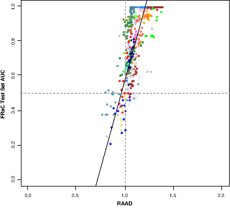
A scatterplot comparing relative anomaly aggregate distance (RAAD) with test set performance over the 28 compendium data sets (each shown in its own color). Points show 20 replicates (random selection of training/test samples) for each data set. Horizontal and vertical lines show an area under the curve (AUC) of 0.5 (random guessing) and a RAAD of 1.0 (normal and anomalous instances equidistant), respectively. (Scatter plots showing individual data sets are available in the Supplementary Material.)

In real applications, where the test data labels are unknown, clinicians' intuition about the degree of expression variation one might expect among the normal class and among the types of envisioned anomalies can be used to estimate whether anomaly detection methods are likely to be helpful. Further, a small test set can be used to estimate the RAAD score, helping to determine the value of obtaining and analyzing additional samples.

3.3. Case studies on fetal and neonatal samples

We applied CSAX to the developmental data sets described in section 2.4. The RAAD scores for the preterm and amniotic fluid data sets were 1.045 and 0.98, respectively. We therefore suspected that it would be impossible to predict abnormalities accurately given the normal amniotic fluid data, and that the presence of preterm complications could be predicted with only moderate accuracy. This hypothesis proved correct. The preterm data set had a CSAX AUC of 0.606 (compared to 0.580, 0.498, and 0.574 with LOF, SVM, and FRaC, respectively); the amniotic fluid data, a CSAX AUC of 0.534 (compared to 0.572, 0.534, and 0.540 with LOF, SVM, and FRaC, respectively). Yet despite the limited overall prediction accuracy, we found the gene sets CSAX highlighted for individuals or groups of samples to be very informative.

3.3.1. Blood from preterm neonates

Only a single neonatal sample had retinopathy of prematurity (ROP) but no other complications. The top gene sets in this sample, with median ranks of 1 and 2 respectively, were “platelet degranulation” and “platelet activation.” ROP, which can lead to vision defects and even blindness, is caused by disordered retinal vascularization. There is an ongoing debate in the literature about whether platelets play a role in the pathogenesis of ROP and what that role might be (Jensen et al., 2011; Vinekar et al., 2010). Our observation of disrupted expression relationships among genes involved in platelet activation in an individual with ROP may provide valuable evidence about the molecular mechanisms of this process.

Our samples also included 14 infants with periventricular leukomalacia (PVL), a type of ischemic brain injury that can lead to cerebral palsy. Glutamate-mediated defects in calcium signaling play a significant role in oligodendrocyte damage in PVL (Butt, 2006) and offer the potential for protective therapeutic intervention (Follett et al., 2004). CSAX highlighted dysregulation of calcium signaling or homeostasis pathways in six individuals with PVL. Such analyses may not only confirm the role of these pathways, but could identify individuals who might be candidates for treatments targeting this process.

3.3.2. Amniotic fluid in aneuploidy and maternal obesity

In the amniotic fluid data set, overall AUC is no better than chance, and indeed CSAX is not the best predictor. The poor RAAD and AUC scores for this data set make sense because the controls are highly variable, including samples collected over a period of more than 6 years. Nonetheless, the gene sets describing the abnormal samples appear to be informative.

The most dysregulated pathway over all abnormal samples together was “regulation of chromosome segregation,” a fitting summary of a data set where 16 of 38 abnormal samples were from fetuses with chromosomal aneupoidy. The most dysregulated pathways in trisomy 21 samples relate to neural development, heart development, and vision; Down syndrome patients are known to have developmental abnormalities in all these systems (Korenberg et al., 1990; McCullough et al., 2013). In trisomy 18, tooth development, immune processes, and glucocorticoid metabolism were among the top ten gene sets, again consistent with prior knowledge about the phenotype (Pont et al., 2006; Turner and O'Herlihy, 1984; Van Dyke and Allen, 1990).

The impact of maternal obesity on fetal development is an active area of research. The top two gene sets implicated by CSAX in these samples overall are “stem cell development” and “stem cell differentiation.” Also highly ranked are “glucose metabolic process” and several gene sets pertaining to nervous system development, including neuronal stem cell maintenance and Notch signaling. Dysregulation of neural stem cells has been noted in the fetal brains of mice fed a high-fat diet (Niculescu and Lupu, 2009; Stachowiak et al., 2013). Additionally, expression of genes involved in Notch signaling, required for neural stem cell development, is known to be disrupted in the brains of offspring of mice fed high fat diets (Yu et al., 2014).

In individual samples we see different processes coming to the fore. One sample featured disruption of lipid and cholesterol transport pathways; in another, axonogenesis was most affected. In two other samples, the top pathways implicated oxidative stress and inflammation. The original analysis of the samples from obese and lean mothers (Edlow et al., 2014) noted that Apolipoprotein D (APOD) is the most upregulated gene in fetuses of obese women. The ApoD protein has been demonstrated to regulate inflammatory response (Do Carmo et al., 2008) and to exert neuroprotective and neurotrophic effects in a rodent model of excitotoxic brain injury, possibly by protecting against oxidative stress (He et al., 2009; Franz et al., 1999; Bajo-Graneras et al., 2011). However, until now, the link between increased expression of APOD and increased oxidative stress in second trimester fetuses of obese women has been only speculative; traditional analyses of these same samples sought but did not find evidence of this connection. Our novel observation may shed light on molecular mechanisms underlying the increased expression of APOD noted in these fetuses, demonstrating how CSAX may provide new insights into the molecular etiology of pathological conditions.

Finally, because maternal BMI is positively correlated with maternal systemic, placental, and neonatal inflammation (Aye et al., 2014), and increased age also correlates positively with systemic inflammation (Franceschi et al., 2000), we reviewed these two patients' clinical characteristics. These two samples are from the patient with the highest maternal age (46 in a cohort with age range 31–46) and one with unusually high BMI (39.5; cohort BMI range: 30.47–39.71). These results strongly suggest that CSAX is identifying valid characteristics of particular samples.

4. Discussion

We have shown that it is often possible to detect and characterize anomalous expression data given training data from normal samples only, and that the two methods designed with expression data in mind perform best, albeit with different strengths. FRaC learns reliable relationships between genes' expression patterns from the training data, and identifies anomalies when these patterns break down. This method is therefore entirely data-driven; it does not rely on prior knowledge about gene sets. Yet it makes sense that many clinically important conditions would be characterized by a breakdown in the expected relationships between genes' expression patterns. So it is perhaps not surprising that FRaC is particularly effective.

On average, CSAX is about as accurate as FRaC (Table 1), but it has two very important differences: it identifies gene sets that may help to explain the nature of each anomaly, and it uses fewer gene expression features in its predictions (because of the discount parameter γ in Eq. 2), instead gaining power from using known gene sets to integrate prior knowledge about gene relationships into the anomaly detection process. We find it revealing that CSAX also outperforms the simple combination of running enrichment analysis on the FRaC anomaly scores (“FRaC + enrichment”). This result suggests that CSAX's bagging and weighting steps succeed in providing the desired robustness.

The identification of gene sets with known functional roles associated with an abnormal sample is one of the primary goals of our work. It provides insight into the nature of the abnormality, and allows experts to follow up by ordering relevant tests. The fact that the performance of CSAX is comparable to that of FRaC while using fewer genes is evidence that the gene sets identified by our method are indeed relevant, because in general the use of fewer features hurts performance.

We also observed that performance depends less on the computational method used than on the difficulty of the data set itself. While the RAAD score is useful for characterizing the difficulty of anomalies whose classification is already known, in most cases such data will not be available. Thus, clinical intuition about the nature of anticipated anomalies will need to come into play. If the anomalous samples are likely to be no more different from the normal samples than the normal samples are from each other, no method is likely to succeed. Prior knowledge about expression variability and heterogeneity of the samples under consideration is expected to be helpful here.

We note that as the cost of sequencing continues to decrease, genome-wide studies of expression are shifting away from microarrays toward RNA-seq approaches. However, there is no reason that CSAX cannot be applied in an RNA-seq setting. Indeed, it might be even more powerful, as changes in the relative abundance of different isoforms can be integrated into the analysis. Future work should therefore include demonstrating CSAX's power to identify systematic anomalies in RNA-seq data.

Overall, we have demonstrated that in many biomedically interesting cases, it is indeed possible to identify and characterize individual anomalous samples from their expression patterns. Such one-of-a-kind analyses are crucial steps as we move toward the era of precision medicine.

Footnotes

Acknowledgments

This research was supported by awards R01-HD-058880 and R01-HD-076140 from the Eunice Kennedy Shriver National Institute of Child Health and Human Development. The content is solely the responsibility of the authors and does not necessarily reflect the views of the NICHD or the National Institutes of Health. Additional support was provided by a Senior Faculty Research Fellowship from Tufts University. The authors thank Pablo Tamayo, George Steinhardt, and Arthur Liberzon for the data behind many of the compendium data sets, and Stan Letovsky and Jill Mesirov for feedback on earlier versions of this work.

Author Disclosure Statement

No competing financial interests exist.

References

Aye

I.L.

, Lager

, Ramirez

V.I.

, et al. 2014. Increasing maternal body mass index is associated with systemic inflammation in the mother and the activation of distinct placental inflammatory pathways. Biol. Reprod., 90, 129.

Bajo-Graneras

, Sanchez

, Gutierrez

, et al. 2011. Apolipoprotein D alters the early transcriptional response to oxidative stress in the adult cerebellum. J. Neurochem., 117, 949–960.

Blake

, Dolan

, Drabkin

, et al. 2012. The Gene Ontology: enhancements for 2012. Nucleic Acids Research, 40, D559–64.

Breunig

, Kriegel

, Ng

, et al. 2000. LOF: identifying density-based local outliers. ACM SIGMOD Record, 29, 93–104.

Butt

A.M.

2006. Neurotransmitter-mediated calcium signalling in oligodendrocyte physiology and pathology. Glia, 54, 666–675.

Chandola

, Banerjee

, and Kumar

2009. Anomaly detection: A survey. ACM Comput. Surv., 41, 15:1–15:58.

Chang

C.-C.

, and Lin

C.-J.

2001. LIBSVM: A library for support vector machines. Software available at http://www.csie.ntu.edu.tw/∼cjlin/libsvm.

Croft

, O'Kelly

, Wu

, et al. 2011. Reactome: a database of reactions, pathways and biological processes. Nucleic Acids Res., 39, D691–D697.

Do Carmo

, Jacomy

, Talbot

P.J.

, and Rassart

2008. Neuroprotective effect of apolipoprotein D against human coronavirus OC43-induced encephalitis in mice. J. Neurosci., 28, 10330–10338.

10.

Dougherty

2001. Small sample issues for microarray-based classification. Comp. Funct. Genomics, 2, 28–34.

11.

Edlow

A.G.

, Vora

N.L.

, Hui

, et al. 2014. Maternal obesity affects fetal neurodevelopmental and metabolic gene expression: A pilot study. PLoS One, 9, e88661.

12.

Follett

P.L.

, Deng

, Dai

, et al. 2004. Glutamate receptor-mediated oligodendrocyte toxicity in periventricular leukomalacia: a protective role for topiramate. J. Neurosci., 24, 4412–4420.

13.

Francavilla

, Cattaneo

, Berezin

, et al. 2009. The binding of ncam to fgfr1 induces a specific cellular response mediated by receptor trafficking. J. Cell. Biol., 187, 1101.

14.

Franceschi

, Bonafe

, Valensin

, et al. 2000. Inflamm-aging. An evolutionary perspective on immunosenescence. Ann. N. Y. Acad. Sci., 908, 244–254.

15.

Franz

, Reindl

, Patel

S.C.

, et al. 1999. Increased expression of apolipoprotein D following experimental traumatic brain injury. J. Neurochem., 73, 1615–1625.

16.

Ghosh

2010. Discrete nonparametric algorithms for outlier detection with genomic data. J. Biopharm. Stat., 20, 193–208.

17.

Glas

A.M.

, Floore

, Delahaye

L.J.

, et al. 2006. Converting a breast cancer microarray signature into a high-throughput diagnostic test. BMC Genomics, 7, 278.

18.

, Jittiwat

, Kim

J.H.

, et al. 2009. Apolipoprotein D modulates F2-isoprostane and 7-ketocholesterol formation and has a neuroprotective effect on organotypic hippocampal cultures after kainate-induced excitotoxic injury. Neurosci. Lett., 455, 183–186.

19.

Hui

, Slonim

, Wick

, et al. 2012. The amniotic fluid transcriptome: a source of novel information about human fetal development. Obstet. Gynecol., 119, 111–8.

20.

Hui

, Wick

H.C.

, Moise

K.J.

, et al. 2013. Global gene expression analysis of amniotic fluid cell-free RNA from recipient twins with twin-twin transfusion syndrome. Prenat. Diagn., 33, 873–883.

21.

Jensen

A.K.

, Ying

G.S.

, Huang

, et al. 2011. Thrombocytopenia and retinopathy of prematurity. J AAPOS, 15, e3–e4.

22.

Kales

, Ryan

, Nau

, et al. 2010. Cbl and human myeloid neoplasms: the Cbl oncogene comes of age. Cancer Res. 70, 4789–94.

23.

Karrila

, Lee

, and Tucker-Kellogg

2011. A comparison of methods for data-driven cancer outlier discovery, and an application scheme to semisupervised predictive biomarker discovery. Cancer Inform., 10, 109–20.

24.

Kim

, and Gelenbe

2009. Anomaly detection in gene expression via stochastic models of gene regulatory networks. BMC Genomics, 10, S26.

25.

Koide

, Slonim

, Johnson

, et al. 2011. Transcriptomic analysis of cell-free fetal RNA suggests a specific molecular phenotype in trisomy 18. Hum. Genet., 129, 295–305.

26.

Korenberg

J.R.

, Kawashima

, Pulst

S.M.

, et al. 1990. Down syndrome: toward a molecular definition of the phenotype. Am. J. Med. Genet. Suppl., 7, 91–97.

27.

, Chaudhuri

, Chant

, and Tang

2007. PADGE: analysis of heterogeneous patterns of differential gene expression. Physiol. Genomics, 32, 154–159.

28.

Lockhart

, Dong

, Byrne

, et al. 1996. Expression monitoring by hybridization to high-density oligonucleotide arrays. Nature Biotech., 14, 1675–80.

29.

Massingham

L.J.

, Johnson

K.L.

, Scholl

T.M.

, et al. 2014. Amniotic fluid RNA gene expression profiling provides insights into the phenotype of Turner syndrome. Hum. Genet., 133, 1075–1082.

30.

McCullough

S.J.

, Little

J.A.

, and Saunders

K.J.

2013. Higher order aberrations in children with Down syndrome. Invest. Ophthalmol. Vis. Sci., 54, 1527–1535.

31.

Mehta

, Jain

, and Badve

2011. Personalized medicine: the road ahead. Clin. Breast Cancer, 11, 20–26.

32.

Mikkelsen

, Galagan

, and Mesirov

2005. Improving genome annotations using phylogenetic profile anomaly detection. Bioinformatics, 21, 464–70.

33.

Mootha

, Lindgren

, Eriksson

K.-F.

, et al. 2003. PGC-1alpha-responsive genes involved in oxidative phosphorylation are coordinately downregulated in human diabetes. Nat. Genet., 34, 267–73.

34.

Mpindi

J.P.

, Sara

, Haapa-Paananen

, et al. 2011. GTI: a novel algorithm for identifying outlier gene expression profiles from integrated microarray datasets. PLoS ONE, 6, e17259.

35.

Niculescu

M.D.

and Lupu

D.S.

2009. High fat diet-induced maternal obesity alters fetal hippocampal development. Int. J. Dev. Neurosci., 27, 627–633.

36.

Noto

, Brodley

, and Slonim

2010. Anomaly detection using an ensemble of feature models. In Proceedings of the 10th IEEE International Conference on Data Mining (ICDM 2010). IEEE Computer Society Press, Washington, DC.

37.

Noto

, Brodley

, and Slonim

2011. FRaC: A feature-modeling approach for semi-supervised and unsupervised anomaly detection. Data Min. Knowl. Discov., 25, 109–133.

38.

Pietrzyk

J.J.

, Kwinta

, Wollen

E.J.

, et al. 2013. Gene expression profiling in preterm infants: new aspects of bronchopulmonary dysplasia development. PLoS ONE, 8, e78585.

39.

Pont

S.J.

, Robbins

J.M.

, Bird

T.M.

, et al. 2006. Congenital malformations among liveborn infants with trisomies 18 and 13. Am. J. Med. Genet. A, 140, 1749–1756.

40.

Sandilands

, Akbarzadeh

, Vecchione

, et al. 2007. Src kinase modulates the activation, transport and signalling dynamics of fibroblast growth factor receptors. EMBO Reports, 8, 1162–1169.

41.

Sauer

, Preininger

, and Hany-Schmatzberger

2005. Quick and simple: quality control of microarray data. Bioinformatics, 21, 1572–1598.

42.

Schölkopf

, Smola

A.J.

, Williamson

R.C.

, et al. 2000. New support vector algorithms. Neural Comput., 12, 1207–1245.

43.

Shalon

, Smith

, and Brown

1996. A DNA micro-array system for analyzing complex DNA samples using two-color fluorescent probe hybridization. Gen. Res., 6, 639–45.

44.

Slonim

2002. From patterns to pathways: gene expression data analysis comes of age. Nat. Genet., 32, 502–508.

45.

Slonim

, Koide

, Johnson

, et al. 2009. Functional genomic analysis of amniotic fluid cell-free mrna suggests that oxidative stress is significant in down syndrome fetuses. PNAS, 106, 9425–9429.

46.

Spackman

K.A.

1989. Signal detection theory: Valuable tools for evaluating inductive learning, 160–163. In Proceedings of the Sixth International Workshop on Machine Learning. Morgan Kaufmann Publishers Inc., San Francisco, CA.

47.

Stachowiak

E.K.

, Oommen

, Vasu

V.T.

, et al. 2013. Maternal obesity affects gene expression and cellular development in fetal brains. Nutr. Neurosci., 16, 96–103.

48.

Subramanian

, Tamayo

, Mootha

V.K.

, et al. 2005. Gene set enrichment analysis: A knowledge-based approach for interpreting genome-wide expression profiles. Proceedings of the National Academy of Sciences, 102, 15545–15550.

49.

Tomlins

, Rhodes

, Perner

, et al. 2005. Recurrent fusion of TMPRSS2 and ETS transcription factor genes in prostate cancer. Science, 310, 644–648.

50.

Torkamani

, and Schork

2009. Prestige centrality-based functional outlier detection in gene expression analysis. Bioinformatics, 25, 2222–2228.

51.

Turner

, and O'Herlihy

1984. Adrenal hypofunction and trisomy 18. Obstet. Gynecol., 63, 84S–85S.

52.

Tusher

, Tibshirani

, and Chu

2001. Significance analysis of microarrays applied to the ionizing radiation response. PNAS, 98, 5116–5121.

53.

Van Dyke

D.C.

, and Allen

1990. Clinical management considerations in long-term survivors with trisomy 18. Pediatrics, 85, 753–759.

54.

Vinekar

, Hegde

, Gilbert

, et al. 2010. Do platelets have a role in the pathogenesis of aggressive posterior retinopathy of prematurity?. Retina, 30, S20–S23.

55.

Wick

H.C.

, Drabkin

, Ngu

, et al. 2014. DFLAT: functional annotation for human development. BMC Bioinformatics, 15, 45.

56.

, Jiang

, Yang

, et al. 2014. Maternal high-fat diet affects Msi/Notch/Hes signaling in neural stem cells of offspring mice. J. Nutr. Biochem., 25, 227–231.

Supplementary Material

Please find the following supplemental material available below.

For Open Access articles published under a Creative Commons License, all supplemental material carries the same license as the article it is associated with.

For non-Open Access articles published, all supplemental material carries a non-exclusive license, and permission requests for re-use of supplemental material or any part of supplemental material shall be sent directly to the copyright owner as specified in the copyright notice associated with the article.

454.98 MB

0.00 MB

CSAX: Characterizing Systematic Anomalies in eXpression Data

Abstract

Abstract

1. Introduction

2. Data and Methods

2.1. Compendium of microarray anomaly detection data sets

2.2. Methods for expression anomaly detection

2.2.1. Prior methods

2.2.2. CSAX: A new method for expression anomaly detection

2.3. Evaluating anomaly detection methods

2.4. Data for developmental case studies

3. Results

3.1. Detection and characterization of anomalous samples

3.2. How hard is an anomaly detection task?

3.3. Case studies on fetal and neonatal samples

3.3.1. Blood from preterm neonates

3.3.2. Amniotic fluid in aneuploidy and maternal obesity

4. Discussion

Footnotes

Acknowledgments

Author Disclosure Statement

References

Supplementary Material