Sage Journals: Discover world-class research

Abstract

Quantitative real-time polymerase chain reaction (qPCR) is a sensitive gene quantification method that has been extensively used in biological and biomedical fields. The currently used methods for PCR data analysis, including the threshold cycle method and linear and nonlinear model-fitting methods, all require subtracting background fluorescence. However, the removal of background fluorescence can hardly be accurate and therefore can distort results. We propose a new method, the taking-difference linear regression method, to overcome this limitation. Briefly, for each two consecutive PCR cycles, we subtract the fluorescence in the former cycle from that in the latter cycle, transforming the n cycle raw data into n−1 cycle data. Then, linear regression is applied to the natural logarithm of the transformed data. Finally, PCR amplification efficiencies and the initial DNA molecular numbers are calculated for each reaction. This taking-difference method avoids the error in subtracting an unknown background, and thus it is more accurate and reliable. This method is easy to perform, and this strategy can be extended to all current methods for PCR data analysis.

1. Introduction

Quantitative real-time polymerase chain reaction (qPCR) has proven to be a powerful tool in molecular biology and biomedical fields to quantify DNA and RNA sequences in research subjects (Heid et al., 1996; Gingeras et al., 2005). The principle of PCR amplification is that double-stranded DNA sequences are amplified exponentially when all the reaction reagents are fresh and available. A real-time PCR kinetic curve starts with the baseline, then enters the exponential amplification phase, followed by the linear phase, and finally ends with the plateau phase (Wilhelm and Pingoud, 2003; Yuan et al., 2006).

There are many methods currently being used to analyze qPCR data, including the threshold cycle (CT) methods that refer to the fractional cycle number at which a certain amount of DNA is reached (Livak and Schmittgen, 2001; Schmittgen and Livak, 2008), the standard curve methods (Rutledge and Cote, 2003; Larionov et al., 2005), linear regression (Peirson et al., 2003; Ramakers et al., 2003), and nonlinear regression models (Schlereth et al., 1998; Liu and Saint, 2002b; Tichopad et al., 2003; Zhao and Fernald, 2005; Guescini et al., 2008). Almost all these methods involve the removal of background fluorescence, or the amount of fluorescence measured before any detectable amplification starts. Background fluorescence may come from unbound fluorochrome, such as SYBR Green I or from fluorochrome bound to double-stranded cDNA and primer annealing to nontarget DNA sequences (Ruijter et al., 2009). Therefore, it is necessary to subtract background fluorescence before applying any analysis method. However, the true value of background fluorescence is unknown, and errors in background correction can lead to significant distortion of the results (Bar et al., 2003; Rutledge, 2004; Larionov et al., 2005; Rebrikov and Trofimov, 2006; Rutledge and Stewart, 2008).

Here, we list three problems caused by background correction. First, incorrect background subtraction leads to miscalculation of PCR efficiency and of the starting gene content (Shain and Clemens, 2008; Ruijter et al., 2009). Taking a set of PCR data as an example, we compared the calculated initial DNA amount and efficiency between the subtraction of the minimum fluorescence and of an average of fluorescence from cycles 3 to 7 by using linear regression-based method. For the background of the minimum, the input DNA amount was 1.04 × 10⁴ and the efficiency was 1.766. For the background of an average, the input DNA amount was 2.96 × 10³, which was closer to the true value of 3.14 × 10³. The efficiency was 1.952. These results reveal a big difference between the two ways of background subtraction. For nonlinear regression methods, the noise of the background fluorescence affects the whole nonlinear curve fitting and identification of the exponential phase (Zhao and Fernald, 2005).

The second issue is that the value of background fluorescence varies when different models are adopted to estimate it. Guescini et al. (2008) fitted five S-shaped models to the PCR curves and did a comparison among them. The fitting of the five models generated the estimates of background ranging from −0.03 to 0.29, as shown in their Table 1.

Table 1.

Equations Used in the Original and the Taking-Difference Linear Regression Methods

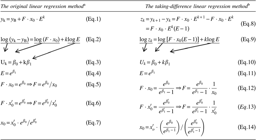
Equation 1 states that the observed fluorescence level after k cycles (y_k) is equal to background fluorescence (y_B) plus the initial DNA molecular numbers (x₀) times F and E^k. F is the conversion factor between the number of target molecules and observed fluorescence. E is amplification efficiency plus one. After taking the natural logarithm on both sides of Eq. 1, we get Eq. 2. Then, we apply linear regression in the form of Eq. 3 and get the formula for calculating E and x₀ as shown in Eqs. 4–7. Eq. 7 is derived from Eq. 5 for a target PCR run and Eq. 6 for a reference run.

Equation 8 indicates that we take the difference of fluorescence for each two consecutive cycles. After taking the natural logarithm on both sides, we get Eq. 9. Similarly, we apply the linear regression model in Eq. 10 and get the formula for calculating E and x₀ as shown in Eqs. 11–14. Equation 14 is derived from Eq. 12 for the target and from Eq. 13 for the reference. By using Eqs. 7 and 14, we calculate the actual initial gene amount in a target run relative to a reference run. In detail, x₀ and \documentclass{aastex}\usepackage{amsbsy}\usepackage{amsfonts}\usepackage{amssymb}\usepackage{bm}\usepackage{mathrsfs}\usepackage{pifont}\usepackage{stmaryrd}\usepackage{textcomp}\usepackage{portland, xspace}\usepackage{amsmath, amsxtra}\pagestyle{empty}\DeclareMathSizes{10}{9}{7}{6}\begin{document} $$x_0^{\prime}$$ \end{document} are the initial gene amounts for target and reference runs, respectively. β₀ and β₁ are the corresponding parameters for a target run, whereas \documentclass{aastex}\usepackage{amsbsy}\usepackage{amsfonts}\usepackage{amssymb}\usepackage{bm}\usepackage{mathrsfs}\usepackage{pifont}\usepackage{stmaryrd}\usepackage{textcomp}\usepackage{portland, xspace}\usepackage{amsmath, amsxtra}\pagestyle{empty}\DeclareMathSizes{10}{9}{7}{6}\begin{document} $$\beta_0^{\prime}$$ \end{document} and \documentclass{aastex}\usepackage{amsbsy}\usepackage{amsfonts}\usepackage{amssymb}\usepackage{bm}\usepackage{mathrsfs}\usepackage{pifont}\usepackage{stmaryrd}\usepackage{textcomp}\usepackage{portland, xspace}\usepackage{amsmath, amsxtra}\pagestyle{empty}\DeclareMathSizes{10}{9}{7}{6}\begin{document} $$\beta_1^{\prime}$$ \end{document} are parameters for the reference.

Finally, it is not always straightforward to define a constant background for all samples within one qPCR run or between different runs. This causes difficulty in comparing varying biological samples (Pfaffl, 2004).

To address all these problems of background correction, we propose a new method called the taking-difference linear regression method, which does not involve background removal. This study also provides a comparison of the taking-difference linear regression method and the original linear regression method with distinct background subtraction. The taking-difference method shows better accuracy and precision. The linear regression model used in both methods enables an estimation of PCR efficiency for each sample without the need to assume the same sample-to-sample efficiency. It also allows for estimating the initial DNA amount for each sample and comparing the DNA start values between samples.

2. Methods

Our idea to avoid background correction is to subtract the fluorescence in the former cycle from that in the latter cycle for each two consecutive PCR cycles, therefore transforming the data from n cycles into n−1 cycles. We illustrate the analysis of such transformed data by the commonly used linear regression method. The detailed equations are shown in Table 1. On the one hand, the original linear regression method was based on a typical exponential function (Eq. 1). It is noticed that background fluorescence is an influential factor in this equation, and it should be subtracted before applying linear regression. The currently used definitions of the background include the mean fluorescence of the first three PCR cycles, the mean of cycles 3–7, and the minimum (Wilhelm et al., 2003b; Larionov et al., 2005; Frank, 2009; Dello Russo et al., 2010). Hence, these three types of background were used in this study for the original linear regression method. Simple linear regression was then applied to the log-transformed function (Eqs. 2 and 3), which had been described previously (Ramakers et al., 2003). On the other hand, the taking-difference linear regression method defines the difference between the fluorescence of two consecutive cycles (Eq. 8). By doing this, background fluorescence is removed. Similarly, simple linear regression model (Eq. 10) was then applied to the log-transformed equation (Eq. 9). For both the original and taking-difference methods, the initial DNA amount (x₀) and amplification efficiency (E−1) can be calculated for each sample using the estimated parameters from linear regression (Eqs. 4–7 and 11–14).

The PCR data set used in the present study was published by Guescini et al. (2008). Briefly, the mitochondrial gene NADH dehydrogenase 1 (MT-ND1) was amplified by qPCR in reactions having a wide range of input DNA molecules (3.14 × 10¹ to 3.14 × 10⁷) in the presence of different amplification mix quantities ranging from 60% to 100%. Within each reaction combination of a specified starting DNA and amplification mix percentage, four separate PCR experiments were conducted, each in triplicate, adding up to a total of 12 runs. PCR experiments were conducted using Light-Cycler 480 SYBR Green I Master (Roche) according to the manufacturer's instructions (Guescini et al., 2008). For the whole data set with 420 PCR runs, the initial DNA molecular number and efficiency were calculated using either the original method or the taking-difference method for each run. Four consecutive cycles with a fluorescence value greater than 0.2 were selected for each run. Here, 0.2 is an arbitrary value between the fluorescence level at the CT and that at the previous cycle. The starting DNA amount in a target PCR run was computed relative to a reference run. The reference groups used for calculations of starting DNA amount were each of the first three runs in the reaction combination of 3.14 × 10⁴ input DNA numbers and 100% amplification mix. The final estimates were the mean of the values generated by using each of the reference runs.

The accuracy of these methods was tested by quantification on samples with known input DNA molecules. Relative errors (REs) were calculated by the following equation: \documentclass{aastex}\usepackage{amsbsy}\usepackage{amsfonts}\usepackage{amssymb}\usepackage{bm}\usepackage{mathrsfs}\usepackage{pifont}\usepackage{stmaryrd}\usepackage{textcomp}\usepackage{portland, xspace}\usepackage{amsmath, amsxtra}\pagestyle{empty}\DeclareMathSizes{10}{9}{7}{6}\begin{document} \begin{align*}RE = \frac {x_0 ^*} {x_0} - 1 ,\end{align*} \end{document}

where \documentclass{aastex}\usepackage{amsbsy}\usepackage{amsfonts}\usepackage{amssymb}\usepackage{bm}\usepackage{mathrsfs}\usepackage{pifont}\usepackage{stmaryrd}\usepackage{textcomp}\usepackage{portland, xspace}\usepackage{amsmath, amsxtra}\pagestyle{empty}\DeclareMathSizes{10}{9}{7}{6}\begin{document} $$x_0^*$$ \end{document} is the estimated initial DNA amount and x₀ is true initial DNA amount. The precision of the methods was analyzed by computing the coefficients of variation (CVs) and mean square errors (MSEs). The equations are shown as follows: \documentclass{aastex}\usepackage{amsbsy}\usepackage{amsfonts}\usepackage{amssymb}\usepackage{bm}\usepackage{mathrsfs}\usepackage{pifont}\usepackage{stmaryrd}\usepackage{textcomp}\usepackage{portland, xspace}\usepackage{amsmath, amsxtra}\pagestyle{empty}\DeclareMathSizes{10}{9}{7}{6}\begin{document} \begin{align*}CV = \frac {s} {\bar {x}} \times 100 , \end{align*} \end{document}

where s and \documentclass{aastex}\usepackage{amsbsy}\usepackage{amsfonts}\usepackage{amssymb}\usepackage{bm}\usepackage{mathrsfs}\usepackage{pifont}\usepackage{stmaryrd}\usepackage{textcomp}\usepackage{portland, xspace}\usepackage{amsmath, amsxtra}\pagestyle{empty}\DeclareMathSizes{10}{9}{7}{6}\begin{document} $$\bar {x}$$ \end{document} are the standard deviation and the mean of a set of observations in each combination of initial gene amount and amplification mix percentage, and \documentclass{aastex}\usepackage{amsbsy}\usepackage{amsfonts}\usepackage{amssymb}\usepackage{bm}\usepackage{mathrsfs}\usepackage{pifont}\usepackage{stmaryrd}\usepackage{textcomp}\usepackage{portland, xspace}\usepackage{amsmath, amsxtra}\pagestyle{empty}\DeclareMathSizes{10}{9}{7}{6}\begin{document} \begin{align*}MSE = \frac {1} {n} \sum_1^n (x_0 ^* - x_0) ^2 ,\end{align*} \end{document}

3. Results

The aim of this study was to compare the accuracy and precision of the initial gene amount estimated using different methods. Therefore, we computed and compared REs, CV, and MSEs. The taking-difference linear regression method was found to be superior to the original linear regression method, with an RE of −0.002 (very close to 0) and CV of 36%, the smallest values among the different methods. Meanwhile, the MSEs by the taking-difference method were generally the smallest for each starting DNA amount (3.14 × 10¹ to 3.14 × 10⁷) compared with other methods (Table 2). This means that the taking-difference linear regression method produces an accurate result with the least variation. The original linear regression method, subtracting cycles 3–7, was the second-best method, with an RE of 0.012 and comparable CV of 48%. The original method with the subtraction of cycles 1–3 gave rise to a larger RE of 0.276 and CV of 60%. The original method, with the minimum subtraction, gave the worst results, with an RE close to 3.0 and CV of 124% (Table 2).

Table 2.

Comparisons Between the Original and the Taking-Difference Linear Regression Methods

	The original linear regression method with background subtraction
	Mean of cycles 1–3				Mean of cycles 3–7				Minimum				The taking-difference linear regression method
DNA molecular number ^a	Estimate ^b	RE	CV	MSE	Estimate	RE	CV	MSE	Estimate	RE	CV	MSE	Estimate	RE	CV	MSE
3.14E+07	4.02E+07	0.280	41.96%	3.66E+14	2.69E+07	−0.144	20.31%	5.52E+13	3.83E+07	0.219	41.96%	4.27E+14	3.20E+07	0.019	32.29%	1.27E+14
3.14E+06	3.21E+06	0.022	33.22%	1.17E+12	3.17E+06	0.009	32.04%	1.10E+12	3.49E+06	0.111	39.91%	3.06E+12	2.85E+06	−0.093	28.90%	9.21E+11
3.14E+05	2.73E+05	−0.130	35.07%	1.11E+10	2.57E+05	−0.181	34.54%	1.15E+10	4.14E+05	0.318	66.90%	1.03E+11	2.63E+05	−0.161	26.49%	8.78E+09
3.14E+04	2.36E+04	−0.248	31.38%	1.17E+08	2.12E+04	−0.326	32.65%	1.55E+08	5.12E+04	0.630	48.44%	1.23E+09	2.76E+04	−0.121	31.17%	1.03E+08
3.14E+03	3.44E+03	0.097	54.00%	3.56E+06	2.96E+03	−0.059	46.90%	2.00E+06	8.62E+03	1.746	103.70%	1.20E+08	3.51E+03	0.118	51.24%	3.61E+06
3.14E+02	9.31E+02	1.965	126.84%	1.76E+06	6.23E+02	0.984	87.30%	3.91E+05	5.38E+03	16.141	410.44%	5.43E+08	3.02E+02	−0.038	36.91%	1.44E+04
3.14E+01	2.97E+01	−0.055	94.44%	7.83E+02	2.51E+01	−0.199	81.92%	4.64E+02	8.44E+01	1.688	153.91%	2.11E+04	3.96E+01	0.262	46.81%	4.42E+02
Mean		0.276	59.56%			0.012	47.95%			2.979	123.61%			−0.002	36.26%

Input DNA molecular numbers.

Estimated DNA molecular numbers.

CV, coefficient of variation; MSE, mean square error; RE, relative error.

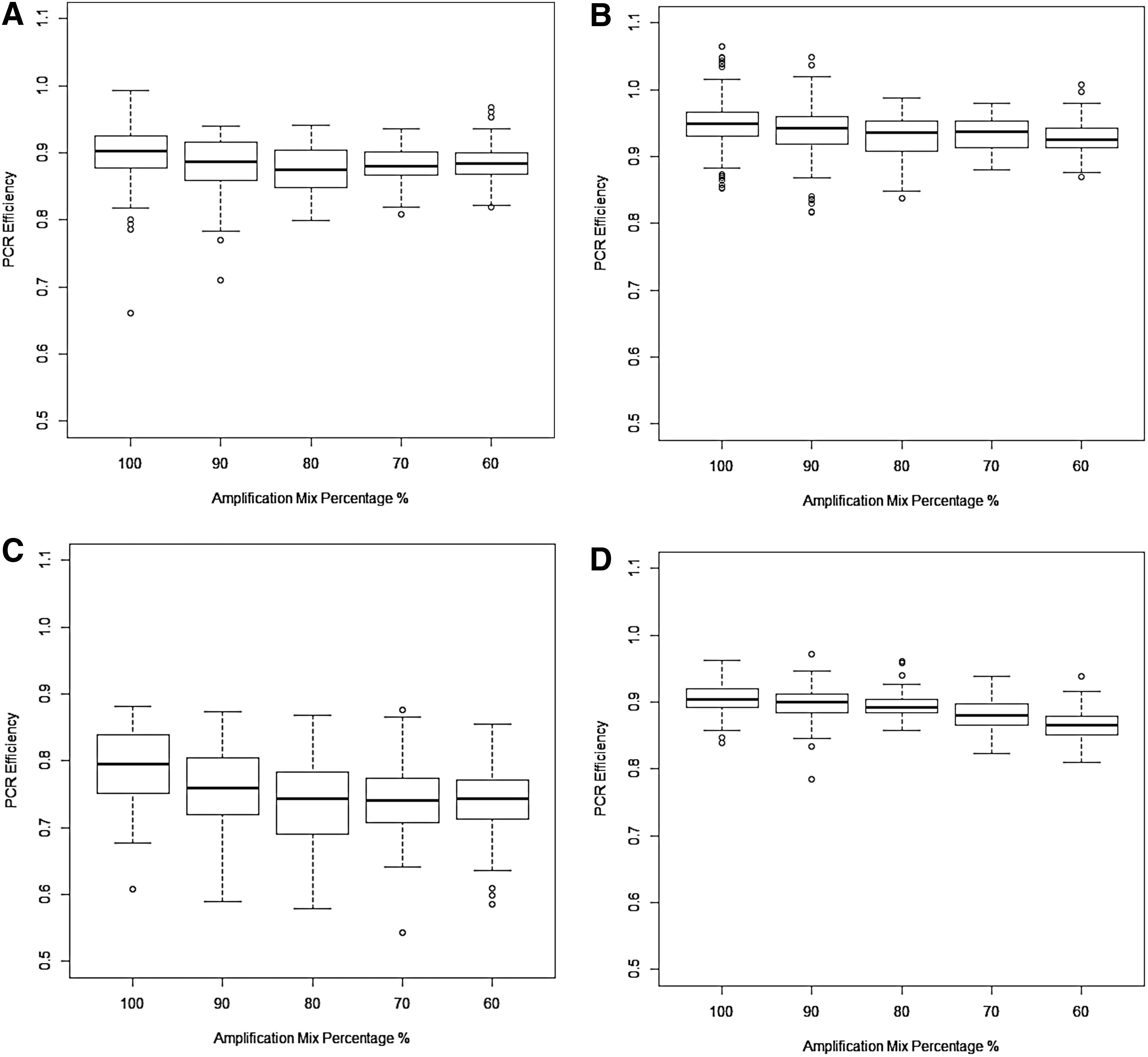
The amplification efficiency was another important parameter to check in qPCR data analysis. It is referred to as E−1. E is any number between 1 and 2, and it is indicated in Equations 1–14 in Table 1. Ideally, the value of E is 2, representing a PCR efficiency of 100% (Higuchi et al., 1993). This means that the number of DNA sequences doubles per cycle under ideal conditions. However, PCR efficiency rarely reaches 100% owing to factors such as reaction inhibitors and differences in probes, enzymes, and primers (Liu and Saint, 2002a; Mygind et al., 2002). It has been suggested that PCR efficiencies range between 80% and 100% (Kamphuis et al., 2001), or between 65% and 90% (Tichopad et al., 2003). The calculated efficiencies for distinct methods are shown in Figure 1, and the detailed summary for both efficiencies and the initial DNA amount is indicated in Table 3. In general, the values of efficiency were the largest, sometimes larger than 100%, when the original method with the subtraction of the mean fluorescence of cycles 3–7 was used. In contrast, the values were the smallest by using the original method with the minimum subtraction. The taking-difference method and the original method (subtracting cycles 1–3) resulted in the efficiency values lie in between. These values seemed to be more reasonable. Theoretically, there should be a monotonically decreasing trend in PCR efficiency for the amplification mix ranging from 100% to 60%. We found that a monotone decrease can be observed only by using the taking-difference method. For the original method with the subtraction of the mean of cycles 1–3, a concave trend was seen with a decrease from 100% to 80% and an increase from 80% to 60%. For the rest, a partial decreasing trend was also seen. In general, the variation was the smallest when the taking-difference method was used (SD = 0.023). Overall, the taking-difference method gave reasonable values and an expected trend of PCR efficiency estimates with the least variation.

FIG. 1.

Comparison of PCR amplification efficiencies estimated using different methods. (A) The original linear regression method with the subtraction of the mean of cycles 1–3. (B) The original linear regression method subtracting the mean of cycles 3–7. (C) The original linear regression method with the minimum subtraction. (D) The taking-difference linear regression method. PCR, polymerase chain reaction.

Table 3.

Summary of Comparisons Between the Original and the Taking-Difference Linear Regression Methods

		The original linear regression method
		Mean of cycles 1–3	Mean of cycles 3–7	Minimum	The taking-difference linear regression method
Amplification efficiency	Overall values	Middle	Largest	Smallest	Middle
	Values >100%	Never	Sometimes	Never	Never
	Change from 100% to 60% amplification mix	Not monotonically decreasing	Not monotonically decreasing	Not monotonically decreasing	Monotonically decreasing
	SD	0.037	0.035	0.061	0.023
Initial DNA amount	RE	Large (up to ∼30%)	Small	Large (up to 300%)	Small
	CV	Up to 60%	Up to ∼50%	Up to ∼120%	Up to ∼35%

SD, standard deviation.

Collectively, the taking-difference linear regression method results in an accurate estimation of the initial DNA amount and a reasonable estimation of amplification efficiencies with the least variation (Table 3). Meanwhile, the original linear regression method with the subtraction of the mean of cycles 3–7 also accurately estimates the initial gene amount but sometimes overestimates PCR efficiencies.

4. Discussion

This study describes a new taking-difference linear regression method for qPCR data analysis and compares it in terms of accuracy and precision with the original linear regression method with multiple background corrections. The taking-difference method is advantageous in several aspects. First, it does not involve the subtraction of background fluorescence. Although most of the analyses rely on the assumption of correct background removal, some other methods have been proposed to relax this assumption. In one study of nonlinear regression, the Real-time PCR Miner method was shown to overcome the limitations of the influence of background fluorescence and to be noise-resistant (Zhao and Fernald, 2005). For linear regression, Ruijter et al. (2009) developed an algorithm that reconstructed the log-linear phase downward from the early plateau phase of the PCR curve to find an estimate of background. The PCR efficiency values of this method were shown to be reproducible. However, the taking-difference method may be superior as it does not involve background correction at all. The second advantage of our method is that it can avoid the extra work of generating a standard curve. Its calculations for all PCR runs can be performed relative to a reference run. Creating a standard curve can be time consuming and requires the concentrations of the standards to be accurate. The errors in sample dilutions and contamination tend to result in an overestimation of PCR efficiency (Peirson et al., 2003). Also, the high consumption of reagents, DNA templates, and experimental material has to be taken into account (Schefe et al., 2006). Additionally, amplification efficiencies need to be assumed to be equal among samples when using methods based on a standard curve. However, this assumption is unreliable in reality (Pfaffl, 2001; Zhao and Fernald, 2005). The third advantage is that it does not require determination of the CT values. Hence, the errors caused by CT estimation can be avoided.

To compare the results obtained by using linear regression and nonlinear regression, we used REs and CV of the estimated initial DNA amount by the original linear regression method and our taking-difference linear regression method, to compare with values obtained by Guescini et al. (2008, their Table 3) using different nonlinear regression methods. We found that our taking-difference method was superior, with a much smaller RE of −0.002 (very close to 0) and comparable CV of 35%. The original linear regression method with the subtraction of cycles 3–7 was also better in terms of a smaller RE (from 0 to 0.1), but the CV was larger than those of the nonlinear regression Cp and Cy₀ methods (∼30–60%).

In general, an appropriate selection of amplification cycles is the key factor for achieving better performance of qPCR analysis methods. Target data points should be within the exponential amplification phase, because the application of linear regression model was based on an exponential equation (Eq. 1; Table 1). Differences in determination of the exponential phase may cause variation in the results (Cikos et al., 2007). There have been several strategies to identify observations within the exponential phase. It has been proposed that the start point should be estimated by the “externally studentized” residual algorithm, whereas the end point by the second derivative maximum value (Tichopad et al., 2003). Another method is to select several cycles with a minimum of three around the midpoint of the fluorescence signal range, because these observations should occur within the exponential phase (Peirson et al., 2003). There are two software packages available to identify the exponential phase of PCR curves (Ramakers et al., 2003; Wilhelm et al., 2003a). In our case, we used PCR threshold to find four consecutive cycles, with the first one being either the rounded CT or the cycle right before it. This strategy of data point selection was based on the general rule that the threshold line is theoretically set above the amplification baseline and within the exponential increase phase (Zhao and Fernald, 2005). In addition, these four target cycles for every PCR run have monotonically increasing fluorescence values. Thus, it is admissible for the logarithm when we use the taking-difference methods by subtracting the fluorescence of the former cycle from the latter one. Moreover, the total number of the data points used among all methods was four. This agrees with previous studies that suggested a selection of 3–5 data points (Bar et al., 2003), 4–6 data points (Ramakers et al., 2003), or 4–10 data points (Zhao and Fernald, 2005). In addition, it has been suggested that using lines with only three data points would give inconsistent starting gene content, whereas longer lines would lead to bias because of inclusion of points not in the exponential phase (Ramakers et al., 2003).

The taking-difference method relies on an assumption that PCR efficiency is constant within the selected cycles in the exponential phase. It has been shown that PCR efficiency is a constant value from the first cycle to the start of the plateau phase (Stolovitzky and Cecchi, 1996). However, it also has been noted that actual PCR efficiency may not be constant throughout an individual reaction (Liu and Saint, 2002b; Platts et al., 2008). The efficiencies may be high during exponential phase and then gradually decrease toward the plateau phase (Gevertz et al., 2005; Zhao and Fernald, 2005; Lalam 2006). They may also be normally distributed (Bar et al., 2003). Since we only used the values of fluorescence for four cycles in the exponential phase, the efficiencies of these four cycles should be very close and can thus be assumed to be equal. This idea was supported by Liu and Saint (2002b). Their simulation revealed that PCR efficiencies during the early exponential phase for a PCR run are relatively constant. To the best of our knowledge, there is no perfect method that is fully assumption-free.

Since PCR data are collected over time, also known as time series data, naturally they have serial correlation/autocorrelation. The serial correlation can be reduced by taking their difference. This is good for fitting linear regression models since the underlying assumption is that the observations are independent of each other.

Overall, the linear-regression-based taking-difference method is of great value for qPCR data analysis in that it is an easy and accurate method that avoids the errors in background subtraction, does not need standard curve generation, and does not assume equal PCR amplification efficiencies between samples.

Footnotes

Acknowledgments

This research was supported by the U.S. National Institutes of Health Grants 5P50 CA100632, 5P01 CA055164, and 1P01 CA108631-01.

Author Disclosure Statement

The authors declare that no competing financial interests exist.

References

Bar

, Stahlberg

, Muszta

, Kubista

2003. Kinetic outlier detection (KOD) in real-time PCR. Nucleic Acids Res., 31:e105.

Cikos

, Bukovska

, Koppel

2007. Relative quantification of mRNA: comparison of methods currently used for real-time PCR data analysis. BMC Mol. Biol., 8:113.

Dello Russo

, Lisi

, Lofaro

et al. 2010. Novel sensitive, specific and rapid pharmacogenomic test for the prediction of abacavir hypersensitivity reaction: HLA-B*57:01 detection by real-time PCR. Pharmacogenomics, 12:567–576.

Frank

D.N.

2009. BARCRAWL and BARTAB: software tools for the design and implementation of barcoded primers for highly multiplexed DNA sequencing. BMC Bioinform., 10:362.

Gevertz

J.L.

, Dunn

S.M.

, Roth

C.M.

2005. Mathematical model of real-time PCR kinetics. Biotechnol. Bioeng., 92:346–355.

Gingeras

T.R.

, Higuchi

, Kricka

L.J.

et al. 2005. Fifty years of molecular (DNA/RNA) diagnostics. Clin. Chem., 51:661–671.

Guescini

, Sisti

, Rocchi

M.B.

et al. 2008. A new real-time PCR method to overcome significant quantitative inaccuracy due to slight amplification inhibition. BMC Bioinform., 9:326.

Heid

C.A.

, Stevens

, Livak

K.J.

, Williams

P.M.

1996. Real time quantitative PCR. Genome Res., 6:986–994.

Higuchi

, Fockler

, Dollinger

, Watson

1993. Kinetic PCR analysis: real-time monitoring of DNA amplification reactions. Biotechnology (N Y), 11:1026–1030.

10.

Kamphuis

, Schneemann

, van Beek

L.M.

et al. 2001. Prostanoid receptor gene expression profile in human trabecular meshwork: a quantitative real-time PCR approach. Invest. Ophthalmol. Vis. Sci., 42:3209–3215.

11.

Lalam

2006. Estimation of the reaction efficiency in polymerase chain reaction. J. Theor. Biol, 242:947–953.

12.

Larionov

, Krause

, Miller

2005. A standard curve based method for relative real time PCR data processing. BMC Bioinform., 6:62.

13.

Liu

, Saint

D.A.

2002a. A new quantitative method of real time reverse transcription polymerase chain reaction assay based on simulation of polymerase chain reaction kinetics. Anal. Biochem., 302:52–59.

14.

Liu

, Saint

D.A.

2002b. Validation of a quantitative method for real time PCR kinetics. Biochem. Biophys. Res. Commun., 294:347–353.

15.

Livak

K.J.

, Schmittgen

T.D.

2001. Analysis of relative gene expression data using real-time quantitative PCR and the 2(-delta delta C(T)) method. Methods, 25:402–408.

16.

Mygind

, Birkelund

, Birkebaek

N.H.

et al. 2002. Determination of PCR efficiency in chelex-100 purified clinical samples and comparison of real-time quantitative PCR and conventional PCR for detection of Chlamydia pneumoniae. BMC Microbiol., 2:17.

17.

Peirson

S.N.

, Butler

J.N.

, Foster

R.G.

2003. Experimental validation of novel and conventional approaches to quantitative real-time PCR data analysis. Nucleic Acids Res., 31:e73.

18.

Pfaffl

M.W.

2001. A new mathematical model for relative quantification in real-time RT-PCR. Nucleic Acids Res., 29:e45.

19.

Pfaffl

M.W.

2004. Quantification strategies in real-time PCR, 87–120. Bustin

S.A.

The Real-Time PCR Encyclopedia A–Z of Quantitative PCR. International University Line: La Jolla, CA.

20.

Platts

A.E.

, Johnson

G.D.

, Linnemann

A.K.

, Krawetz

S.A.

2008. Real-time PCR quantification using a variable reaction efficiency model. Anal. Biochem., 380:315–322.

21.

Ramakers

, Ruijter

J.M.

, Deprez

R.H.

, Moorman

A.F.

2003. Assumption-free analysis of quantitative real-time polymerase chain reaction (PCR) data. Neurosci. Lett., 339:62–66.

22.

Rebrikov

D.V.

, Trofimov

2006. [Real-time PCR: approaches to data analysis (a review)] Prikl. Biokhim. Mikrobiol., 42:520–528.

23.

Ruijter

J.M.

, Ramakers

, Hoogaars

W.M.

et al. 2009. Amplification efficiency: linking baseline and bias in the analysis of quantitative PCR data. Nucleic Acids Res., 37:e45.

24.

Rutledge

R.G.

2004. Sigmoidal curve-fitting redefines quantitative real-time PCR with the prospective of developing automated high-throughput applications. Nucleic Acids Res., 32:e178.

25.

Rutledge

R.G.

, Cote

2003. Mathematics of quantitative kinetic PCR and the application of standard curves. Nucleic Acids Res., 31:e93.

26.

Rutledge

R.G.

, Stewart

2008. A kinetic-based sigmoidal model for the polymerase chain reaction and its application to high-capacity absolute quantitative real-time PCR. BMC Biotechnol., 8:47.

27.

Schefe

J.H.

, Lehmann

K.E.

, Buschmann

I.R.

et al. 2006. Quantitative real-time RT-PCR data analysis: current concepts and the novel “gene expression's CT difference” formula. J. Mol. Med. (Berl.), 84:901–910.

28.

Schlereth

, Bassukas

I.D.

, Deubel

et al. 1998. Use of the recursion formula of the Gompertz function for the quantitation of PCR-amplified templates. Int. J. Mol. Med, 1:463–467.

29.

Schmittgen

T.D.

, Livak

K.J.

2008. Analyzing real-time PCR data by the comparative C(T) method. Nat. Protoc., 3:1101–1108.

30.

Shain

E.B.

, Clemens

J.M.

2008. A new method for robust quantitative and qualitative analysis of real-time PCR. Nucleic Acids Res., 36:e91.

31.

Stolovitzky

, Cecchi

1996. Efficiency of DNA replication in the polymerase chain reaction. Proc. Natl. Acad. Sci. U. S. A., 93:12947–12952.

32.

Tichopad

, Dilger

, Schwarz

, Pfaffl

M.W.

2003. Standardized determination of real-time PCR efficiency from a single reaction set-up. Nucleic Acids Res., 31:e122.

33.

Wilhelm

, Pingoud

2003. Real-time polymerase chain reaction. Chem. Biochem., 4:1120–1128.

34.

Wilhelm

, Pingoud

, Hahn

2003a. SoFAR: software for fully automatic evaluation of real-time PCR data. Biotechniques, 34:324–332.

35.

Wilhelm

, Pingoud

, Hahn

2003b. Validation of an algorithm for automatic quantification of nucleic acid copy numbers by real-time polymerase chain reaction. Anal. Biochem., 317:218–225.

36.

Yuan

J.S.

, Reed

, Chen

, Stewart

C.N.

Jr . 2006. Statistical analysis of real-time PCR data. BMC Bioinform., 7:85.

37.

Zhao

, Fernald

R.D.

2005. Comprehensive algorithm for quantitative real-time polymerase chain reaction. J. Comput. Biol., 12:1047–1064.

A New Method for Quantitative Real-Time Polymerase Chain Reaction Data Analysis

Abstract

Abstract

1. Introduction

2. Methods

3. Results

4. Discussion

Footnotes

Acknowledgments

Author Disclosure Statement

References