Contemporary practical methods for protein nuclear magnetic resonance (NMR) structure determination use molecular dynamics coupled with a simulated annealing schedule. The objective of these methods is to minimize the error of deviating from the nuclear overhauser effect (NOE) distance constraints. However, the corresponding objective function is highly nonconvex and, consequently, difficult to optimize. Euclidean distance matrix (EDM) methods based on semidefinite programming (SDP) provide a natural framework for these problems. However, the high complexity of SDP solvers and the often noisy distance constraints provide major challenges to this approach. The main contribution of this article is a new SDP formulation for the EDM approach that overcomes these two difficulties. We model the protein as a set of intersecting two- and three-dimensional cliques. Then, we adapt and extend a technique called semidefinite facial reduction to reduce the SDP problem size to approximately one quarter of the size of the original problem. The reduced SDP problem can be solved approximately 100 times faster, and it is also more resistant to numerical problems from erroneous and inexact distance bounds.
1. Introduction
Computing three-dimensional 3D protein structures from their amino acid sequences is one of the most widely studied problems in bioinformatics. Knowing the structure of the protein is key to understanding its physical, chemical, and biological properties. The protein nuclear magnetic resonance (NMR) method is fundamentally different from the X-ray method: It is not a “microscope with atomic resolution”; rather, it provides a network of distance measurements between spatially proximate hydrogen atoms (Güntert, 1998). As a result, the NMR method relies heavily on complex computational algorithms. The existing methods for protein NMR can be categorized into four major groups: (i) methods based on Euclidean distance matrix completion (EDMC) (Braun et al., 1981; Havel and Wüthrich, 1984; Biswas et al., 2008; Leung and Toh, 2009); (ii) methods based on molecular dynamics and simulated annealing (Nilges et al., 1988; Brünger, 1993; Güntert et al., 1997; Schwieters et al., 2003; Güntert, 2004); (iii) methods based on local/global optimization (Braun and Go, 1985; Moré and Wu, 1997; Williams et al., 2001); and (iv) methods originating from sequence-based protein structure prediction algorithms (Shen et al., 2008; Raman et al., 2010; Alipanahi et al., 2011).
In the early years of protein NMR, many EDMC-based methods directly worked on the corresponding Euclidean distance matrix (EDM). The first method to use EDMC for protein NMR was developed by Braun et al. (1981). Other notable methods include EMBED (Havel et al., 1983) and DISGEO (Havel and Wüthrich, 1984). These methods faced two major drawbacks: randomly guessing the unknown distances is ineffective and after several iterations of distance correction, the error in the distances tended to become large (Güntert, 1998); and there was no way to control the embedding dimensionality, which also tended to become large.
A major breakthrough came that combined simulated annealing with molecular dynamics (MD) simulation. Nilges et al. (1998) made some improvements in the MD-based protein NMR structure determination. Instead of an empirical energy function, they proposed a simple geometrical energy function based on the NOE restraints that penalized large violations, and they also combined simulated annealing (SA) with MD. These methods were able to search the massive conformation space without being trapped in one of numerous local minima. The XPLOR method (Brünger, 1993; Schwieters et al., 2003, 2006) was one of the first successful and widely adapted methods that was built on the molecular dynamics simulation package CHARMM (Brooks et al., 1983). The number of degrees of freedom in torsion angle space is nearly 10 times smaller than in Cartesian coordinates space, while being equivalent under mild assumptions. The torsion angle dynamics algorithm implemented in the program CYANA (Güntert, 2004), and previously in the program DYANA (Güntert et al., 1997), is one of the fastest and most widely used methods.
1.1. Gram matrix methods
The EDMC methods are based on using the Gram matrix, or the matrix of inner products. This has many advantages. For example, (i) the Gram matrix and Euclidean distance matrix (EDM) are linearly related; (ii) instead of enforcing all of the triangle inequality constraints, it is sufficient to enforce that the Gram matrix is positive semidefinite; and (iii) the embedding dimension and the rank of the Gram matrix are directly related.
Semidefinite programming (SDP) is a natural choice for formulating the EDMC problem using the Gram matrix. SDP-based EDMC methods have demonstrated great success in solving the sensor network localization (SNL) problem (Doherty et al., 2001; Biswas and Ye, 2004; Biswas et al., 2006; Wang et al., 2008; Kim et al., 2009; Krislock and Wolkowicz, 2010). In the SNL problem, the location of a set of sensors is determined based on given short-range distances between spatially proximate sensors. As a result, the SNL problem is inherently similar to the protein NMR problem. The major obstacle in extending SNL methods to protein NMR is the complexity of SDP solvers. To overcome this limitation, Biswas et al. (2008) proposed DAFGAL, which is built on the idea of divide-and-stitch. Leung and Toh (2009) proposed the DISCO method. It is an extension of DAFGAL that can determine protein molecules with more than 10,000 atoms using a divide-and-conquer technique. The improved methods for partitioning the partial distance matrix and iteratively aligning the solutions of the subproblems boosted the performance of DISCO in comparison to DAFGAL.
1.2. Contributions of the proposed SPROS method
Most of the existing methods make some of the following assumptions: (i) (nearly) exact distances between atoms are known; (ii) distances between any type of nuclei (not just hydrogens) are known; (iii) ignoring the fact that not all hydrogen atoms can be uniquely assigned; and (iv) overlooking the ambiguity in the NOE cross-peak assignments. In order to automate the NMR protein structure determination process, we need a robust structure calculation method that tolerates more errors. In this article, we give a new SDP formulation that does not assume (i–iv) above. Moreover, the new method, called “SPROS” (semidefinite programming-based protein structure determination), models the protein molecule as a set of intersecting two- and three-dimension cliques. We adapt and extend a technique called semidefinite facial reduction, which makes the SDP problem strictly feasible and reduces its size to approximately one quarter the size of the original problem. The reduced problem is more numerically stable and can be solved nearly 100 times faster.
Outline We have divided the presentation of the SPROS method into providing the necessary background, followed by giving a description of techniques used for problem size reduction, and finally, showing the performance of the method on experimentally derived data.
Preliminaries Scalars, vectors, sets, and matrices are shown in lowercase, lowercase bold italic, script, and uppercase italic letters, respectively. We work only on real finite-dimensional Euclidean Spaces\documentclass{aastex}\usepackage{amsbsy}\usepackage{amsfonts}\usepackage{amssymb}\usepackage{bm}\usepackage{mathrsfs}\usepackage{pifont}\usepackage{stmaryrd}\usepackage{textcomp}\usepackage{portland, xspace}\usepackage{amsmath, amsxtra}\pagestyle{empty}\DeclareMathSizes{10}{9}{7}{6}\begin{document}
$${\mathbb E}$$
\end{document} and define an inner product operator \documentclass{aastex}\usepackage{amsbsy}\usepackage{amsfonts}\usepackage{amssymb}\usepackage{bm}\usepackage{mathrsfs}\usepackage{pifont}\usepackage{stmaryrd}\usepackage{textcomp}\usepackage{portland, xspace}\usepackage{amsmath, amsxtra}\pagestyle{empty}\DeclareMathSizes{10}{9}{7}{6}\begin{document}
$$\langle \cdot , \cdot \rangle:{\mathbb E} \times {\mathbb E}
\rightarrow{\mathbb R}$$
\end{document} for these spaces: (i) for the space of real p-dimensional vectors, \documentclass{aastex}\usepackage{amsbsy}\usepackage{amsfonts}\usepackage{amssymb}\usepackage{bm}\usepackage{mathrsfs}\usepackage{pifont}\usepackage{stmaryrd}\usepackage{textcomp}\usepackage{portland, xspace}\usepackage{amsmath, amsxtra}\pagestyle{empty}\DeclareMathSizes{10}{9}{7}{6}\begin{document}
$${\mathbb R}^p , \langle \textbf{\textit{x , y}} \rangle: =
\textbf{\textit{x}}^ \top \textbf{\textit{y}} = \sum\nolimits_{i =
1}^p \textbf{\textit{x}}_i \textbf{\textit{y}}_i
$$
\end{document}, and (ii) for the space of real p × q matrices, \documentclass{aastex}\usepackage{amsbsy}\usepackage{amsfonts}\usepackage{amssymb}\usepackage{bm}\usepackage{mathrsfs}\usepackage{pifont}\usepackage{stmaryrd}\usepackage{textcomp}\usepackage{portland, xspace}\usepackage{amsmath, amsxtra}\pagestyle{empty}\DeclareMathSizes{10}{9}{7}{6}\begin{document}
$${\mathbb R}^{p \times q} , \langle A , B \rangle : = {\bf trace}
(A^ \top B) = \sum\nolimits_{i = 1}^p \sum\nolimits_{j = 1}^q
A_{ij} B_{ij}$$
\end{document}. The Euclidean distance norm of \documentclass{aastex}\usepackage{amsbsy}\usepackage{amsfonts}\usepackage{amssymb}\usepackage{bm}\usepackage{mathrsfs}\usepackage{pifont}\usepackage{stmaryrd}\usepackage{textcomp}\usepackage{portland, xspace}\usepackage{amsmath, amsxtra}\pagestyle{empty}\DeclareMathSizes{10}{9}{7}{6}\begin{document}
$$\textbf{\textit{x}} \in {\mathbb R}^p$$
\end{document} is defined as \documentclass{aastex}\usepackage{amsbsy}\usepackage{amsfonts}\usepackage{amssymb}\usepackage{bm}\usepackage{mathrsfs}\usepackage{pifont}\usepackage{stmaryrd}\usepackage{textcomp}\usepackage{portland, xspace}\usepackage{amsmath, amsxtra}\pagestyle{empty}\DeclareMathSizes{10}{9}{7}{6}\begin{document}
$$\mid \mid \textbf{\textit{x}} \mid \mid : = \sqrt{\langle
\textbf{\textit{x}} , \textbf{\textit{x}} \rangle}$$
\end{document}. We use the Matlab notation that \documentclass{aastex}\usepackage{amsbsy}\usepackage{amsfonts}\usepackage{amssymb}\usepackage{bm}\usepackage{mathrsfs}\usepackage{pifont}\usepackage{stmaryrd}\usepackage{textcomp}\usepackage{portland, xspace}\usepackage{amsmath, amsxtra}\pagestyle{empty}\DeclareMathSizes{10}{9}{7}{6}\begin{document}
$$1 : n: = \{1 , 2 , \ldots , n \} $$
\end{document}. For a matrix \documentclass{aastex}\usepackage{amsbsy}\usepackage{amsfonts}\usepackage{amssymb}\usepackage{bm}\usepackage{mathrsfs}\usepackage{pifont}\usepackage{stmaryrd}\usepackage{textcomp}\usepackage{portland, xspace}\usepackage{amsmath, amsxtra}\pagestyle{empty}\DeclareMathSizes{10}{9}{7}{6}\begin{document}
$$A \in {\mathbb R}^{n \times n}$$
\end{document} and an index set\documentclass{aastex}\usepackage{amsbsy}\usepackage{amsfonts}\usepackage{amssymb}\usepackage{bm}\usepackage{mathrsfs}\usepackage{pifont}\usepackage{stmaryrd}\usepackage{textcomp}\usepackage{portland, xspace}\usepackage{amsmath, amsxtra}\pagestyle{empty}\DeclareMathSizes{10}{9}{7}{6}\begin{document}
$${\cal I} \subseteq 1{:}n , B = A [{\cal I}]$$
\end{document} is the \documentclass{aastex}\usepackage{amsbsy}\usepackage{amsfonts}\usepackage{amssymb}\usepackage{bm}\usepackage{mathrsfs}\usepackage{pifont}\usepackage{stmaryrd}\usepackage{textcomp}\usepackage{portland, xspace}\usepackage{amsmath, amsxtra}\pagestyle{empty}\DeclareMathSizes{10}{9}{7}{6}\begin{document}
$$\mid {\cal I} \mid \times \mid {\cal I} \mid$$
\end{document} matrix formed by rows and columns of A indexed by \documentclass{aastex}\usepackage{amsbsy}\usepackage{amsfonts}\usepackage{amssymb}\usepackage{bm}\usepackage{mathrsfs}\usepackage{pifont}\usepackage{stmaryrd}\usepackage{textcomp}\usepackage{portland, xspace}\usepackage{amsmath, amsxtra}\pagestyle{empty}\DeclareMathSizes{10}{9}{7}{6}\begin{document}
$${\cal I}$$
\end{document}. Finally, we let \documentclass{aastex}\usepackage{amsbsy}\usepackage{amsfonts}\usepackage{amssymb}\usepackage{bm}\usepackage{mathrsfs}\usepackage{pifont}\usepackage{stmaryrd}\usepackage{textcomp}\usepackage{portland, xspace}\usepackage{amsmath, amsxtra}\pagestyle{empty}\DeclareMathSizes{10}{9}{7}{6}\begin{document}
$${\cal S}^p$$
\end{document} the space of symmetric p × p matrices.
2. The SPROS Method
2.1. Euclidean distance geometry
Euclidean Distance Matrix A symmetric matrix D is called a Euclidean distance matrix (EDM) if there exists a set of points \documentclass{aastex}\usepackage{amsbsy}\usepackage{amsfonts}\usepackage{amssymb}\usepackage{bm}\usepackage{mathrsfs}\usepackage{pifont}\usepackage{stmaryrd}\usepackage{textcomp}\usepackage{portland, xspace}\usepackage{amsmath, amsxtra}\pagestyle{empty}\DeclareMathSizes{10}{9}{7}{6}\begin{document}
$$\{\textbf{\textit{x}}_\textbf{\textit{1}} , \ldots ,
\textbf{\textit{x}}_\textbf{\textit{n}} \} ,
\textbf{\textit{x}}_\textbf{\textit{i}} \in{\mathbb R}^r$$
\end{document} such that:
\documentclass{aastex}\usepackage{amsbsy}\usepackage{amsfonts}\usepackage{amssymb}\usepackage{bm}\usepackage{mathrsfs}\usepackage{pifont}\usepackage{stmaryrd}\usepackage{textcomp}\usepackage{portland, xspace}\usepackage{amsmath, amsxtra}\pagestyle{empty}\DeclareMathSizes{10}{9}{7}{6}\begin{document}
\begin{align*}D_{ij} = \parallel \textbf{\textit{x}}_i -
\textbf{\textit{x}}_j \parallel ^2 , \quad \forall i , j.
\tag{1}\end{align*}
\end{document}
The smallest value of r is called the embedding dimension of D, and is denoted embdim(D). The space of all n × n EDMs is denoted \documentclass{aastex}\usepackage{amsbsy}\usepackage{amsfonts}\usepackage{amssymb}\usepackage{bm}\usepackage{mathrsfs}\usepackage{pifont}\usepackage{stmaryrd}\usepackage{textcomp}\usepackage{portland, xspace}\usepackage{amsmath, amsxtra}\pagestyle{empty}\DeclareMathSizes{10}{9}{7}{6}\begin{document}
$${\cal E}^n$$
\end{document}.
The Gram Matrix If we define \documentclass{aastex}\usepackage{amsbsy}\usepackage{amsfonts}\usepackage{amssymb}\usepackage{bm}\usepackage{mathrsfs}\usepackage{pifont}\usepackage{stmaryrd}\usepackage{textcomp}\usepackage{portland, xspace}\usepackage{amsmath, amsxtra}\pagestyle{empty}\DeclareMathSizes{10}{9}{7}{6}\begin{document}
$$X : = [\textbf{\textit{x}}_1 , \ldots , \textbf{\textit{x}}_n]
\in {\mathbb R}^{r \times n}$$
\end{document}, then the matrix of inner-products, or Gram matrix, is given by \documentclass{aastex}\usepackage{amsbsy}\usepackage{amsfonts}\usepackage{amssymb}\usepackage{bm}\usepackage{mathrsfs}\usepackage{pifont}\usepackage{stmaryrd}\usepackage{textcomp}\usepackage{portland, xspace}\usepackage{amsmath, amsxtra}\pagestyle{empty}\DeclareMathSizes{10}{9}{7}{6}\begin{document}
$$G: = X^{\top}X$$
\end{document}. It immediately follows that \documentclass{aastex}\usepackage{amsbsy}\usepackage{amsfonts}\usepackage{amssymb}\usepackage{bm}\usepackage{mathrsfs}\usepackage{pifont}\usepackage{stmaryrd}\usepackage{textcomp}\usepackage{portland, xspace}\usepackage{amsmath, amsxtra}\pagestyle{empty}\DeclareMathSizes{10}{9}{7}{6}\begin{document}
$$G \in {\cal S}_+^n$$
\end{document}, where \documentclass{aastex}\usepackage{amsbsy}\usepackage{amsfonts}\usepackage{amssymb}\usepackage{bm}\usepackage{mathrsfs}\usepackage{pifont}\usepackage{stmaryrd}\usepackage{textcomp}\usepackage{portland, xspace}\usepackage{amsmath, amsxtra}\pagestyle{empty}\DeclareMathSizes{10}{9}{7}{6}\begin{document}
$${{\cal S}_+ ^n}$$
\end{document} is the set of symmetric positive semidefinite n × n matrices. The Gram matrix and the Euclidean distance matrix are linearly related:
\documentclass{aastex}\usepackage{amsbsy}\usepackage{amsfonts}\usepackage{amssymb}\usepackage{bm}\usepackage{mathrsfs}\usepackage{pifont}\usepackage{stmaryrd}\usepackage{textcomp}\usepackage{portland, xspace}\usepackage{amsmath, amsxtra}\pagestyle{empty}\DeclareMathSizes{10}{9}{7}{6}\begin{document}
\begin{align*}D = {\rm K} (G) : = {\bf diag} (G) \cdot{\bf
1}^ \top + {\bf 1} \cdot {\bf diag} (G) ^ \top - 2G ,
\tag{2}\end{align*}
\end{document}
where 1 is the all-ones vector of the appropriate size, and diag(G) is the vector formed from the diagonal of G. To go from the EDM to the Gram matrix, we use the Moore-Penrose generalized inverse \documentclass{aastex}\usepackage{amsbsy}\usepackage{amsfonts}\usepackage{amssymb}\usepackage{bm}\usepackage{mathrsfs}\usepackage{pifont}\usepackage{stmaryrd}\usepackage{textcomp}\usepackage{portland, xspace}\usepackage{amsmath, amsxtra}\pagestyle{empty}\DeclareMathSizes{10}{9}{7}{6}\begin{document}
$${\rm K}^ \dag: {\cal S}^n \rightarrow {\cal S}^n :$$
\end{document}\documentclass{aastex}\usepackage{amsbsy}\usepackage{amsfonts}\usepackage{amssymb}\usepackage{bm}\usepackage{mathrsfs}\usepackage{pifont}\usepackage{stmaryrd}\usepackage{textcomp}\usepackage{portland, xspace}\usepackage{amsmath, amsxtra}\pagestyle{empty}\DeclareMathSizes{10}{9}{7}{6}\begin{document}
\begin{align*}G = {\rm K} ^ \dag (D) : = - \frac {1} {2}
HDH , \quad D \in {\cal S} _H^n , \tag {3} \end{align*}
\end{document}
where \documentclass{aastex}\usepackage{amsbsy}\usepackage{amsfonts}\usepackage{amssymb}\usepackage{bm}\usepackage{mathrsfs}\usepackage{pifont}\usepackage{stmaryrd}\usepackage{textcomp}\usepackage{portland, xspace}\usepackage{amsmath, amsxtra}\pagestyle{empty}\DeclareMathSizes{10}{9}{7}{6}\begin{document}
$$H = I - \frac {1} {n} {\bf 11} ^ \top$$
\end{document} is the centering matrix, and \documentclass{aastex}\usepackage{amsbsy}\usepackage{amsfonts}\usepackage{amssymb}\usepackage{bm}\usepackage{mathrsfs}\usepackage{pifont}\usepackage{stmaryrd}\usepackage{textcomp}\usepackage{portland, xspace}\usepackage{amsmath, amsxtra}\pagestyle{empty}\DeclareMathSizes{10}{9}{7}{6}\begin{document}
$${\cal S}_H^n : = \{A \in {\cal S}^n : {\bf diag} (A) = {
\bf 0} \} $$
\end{document} is the set of symmetric matrices with zero diagonal.
Schoenberg's Theorem Given a matrix D, we can determine if it is an EDM with the following well-known theorem (Schoenberg, 1935):
Theorem 1
A matrix\documentclass{aastex}\usepackage{amsbsy}\usepackage{amsfonts}\usepackage{amssymb}\usepackage{bm}\usepackage{mathrsfs}\usepackage{pifont}\usepackage{stmaryrd}\usepackage{textcomp}\usepackage{portland, xspace}\usepackage{amsmath, amsxtra}\pagestyle{empty}\DeclareMathSizes{10}{9}{7}{6}\begin{document}
$$D \in {\cal S}_H^n$$
\end{document}is a Euclidean distance matrix if and only if K†(D) is positive semidefinite. Moreover,embdim(D) = rank(K†(D)), for all\documentclass{aastex}\usepackage{amsbsy}\usepackage{amsfonts}\usepackage{amssymb}\usepackage{bm}\usepackage{mathrsfs}\usepackage{pifont}\usepackage{stmaryrd}\usepackage{textcomp}\usepackage{portland, xspace}\usepackage{amsmath, amsxtra}\pagestyle{empty}\DeclareMathSizes{10}{9}{7}{6}\begin{document}
$$D \in {\cal E}^n$$
\end{document}.
2.2. The SDP formulation
Semidefinite optimization or, more commonly, semidefinite programming, is a class of convex optimization problems that has attracted much attention in the optimization community and has found numerous applications in different science and engineering fields. Notably, several diverse convex optimization problems can be formulated as SDP problems (Vandenberghe and Boyd, 1996). Current state-of-the-art SDP solvers are based on primal-dual interior-point methods.
Preliminary Problem Formulation There are three types of constraints in our formulation: (i) equality constraints, which are the union of equality constraints preserving bond lengths (\documentclass{aastex}\usepackage{amsbsy}\usepackage{amsfonts}\usepackage{amssymb}\usepackage{bm}\usepackage{mathrsfs}\usepackage{pifont}\usepackage{stmaryrd}\usepackage{textcomp}\usepackage{portland, xspace}\usepackage{amsmath, amsxtra}\pagestyle{empty}\DeclareMathSizes{10}{9}{7}{6}\begin{document}
$${\cal B}$$
\end{document}), bond angles (\documentclass{aastex}\usepackage{amsbsy}\usepackage{amsfonts}\usepackage{amssymb}\usepackage{bm}\usepackage{mathrsfs}\usepackage{pifont}\usepackage{stmaryrd}\usepackage{textcomp}\usepackage{portland, xspace}\usepackage{amsmath, amsxtra}\pagestyle{empty}\DeclareMathSizes{10}{9}{7}{6}\begin{document}
$${\cal A}$$
\end{document}), and planarity of the coplanar atoms (\documentclass{aastex}\usepackage{amsbsy}\usepackage{amsfonts}\usepackage{amssymb}\usepackage{bm}\usepackage{mathrsfs}\usepackage{pifont}\usepackage{stmaryrd}\usepackage{textcomp}\usepackage{portland, xspace}\usepackage{amsmath, amsxtra}\pagestyle{empty}\DeclareMathSizes{10}{9}{7}{6}\begin{document}
$${\cal P}$$
\end{document}), giving \documentclass{aastex}\usepackage{amsbsy}\usepackage{amsfonts}\usepackage{amssymb}\usepackage{bm}\usepackage{mathrsfs}\usepackage{pifont}\usepackage{stmaryrd}\usepackage{textcomp}\usepackage{portland, xspace}\usepackage{amsmath, amsxtra}\pagestyle{empty}\DeclareMathSizes{10}{9}{7}{6}\begin{document}
$${\cal E} = {\cal E}_{\cal B} \cup{\cal E}_{\cal A} \cup {\cal E}_{\cal P}$$
\end{document}; (ii) upper bounds, which are the union of NOE-derived (\documentclass{aastex}\usepackage{amsbsy}\usepackage{amsfonts}\usepackage{amssymb}\usepackage{bm}\usepackage{mathrsfs}\usepackage{pifont}\usepackage{stmaryrd}\usepackage{textcomp}\usepackage{portland, xspace}\usepackage{amsmath, amsxtra}\pagestyle{empty}\DeclareMathSizes{10}{9}{7}{6}\begin{document}
$${\cal N}$$
\end{document}), hydrogen bonds (\documentclass{aastex}\usepackage{amsbsy}\usepackage{amsfonts}\usepackage{amssymb}\usepackage{bm}\usepackage{mathrsfs}\usepackage{pifont}\usepackage{stmaryrd}\usepackage{textcomp}\usepackage{portland, xspace}\usepackage{amsmath, amsxtra}\pagestyle{empty}\DeclareMathSizes{10}{9}{7}{6}\begin{document}
$${\cal H}$$
\end{document}), disulfide and salt bridges (\documentclass{aastex}\usepackage{amsbsy}\usepackage{amsfonts}\usepackage{amssymb}\usepackage{bm}\usepackage{mathrsfs}\usepackage{pifont}\usepackage{stmaryrd}\usepackage{textcomp}\usepackage{portland, xspace}\usepackage{amsmath, amsxtra}\pagestyle{empty}\DeclareMathSizes{10}{9}{7}{6}\begin{document}
$${\cal D}$$
\end{document}), and torsion angle (\documentclass{aastex}\usepackage{amsbsy}\usepackage{amsfonts}\usepackage{amssymb}\usepackage{bm}\usepackage{mathrsfs}\usepackage{pifont}\usepackage{stmaryrd}\usepackage{textcomp}\usepackage{portland, xspace}\usepackage{amsmath, amsxtra}\pagestyle{empty}\DeclareMathSizes{10}{9}{7}{6}\begin{document}
$${\cal T}$$
\end{document}) upper bounds, giving \documentclass{aastex}\usepackage{amsbsy}\usepackage{amsfonts}\usepackage{amssymb}\usepackage{bm}\usepackage{mathrsfs}\usepackage{pifont}\usepackage{stmaryrd}\usepackage{textcomp}\usepackage{portland, xspace}\usepackage{amsmath, amsxtra}\pagestyle{empty}\DeclareMathSizes{10}{9}{7}{6}\begin{document}
$${\cal U} = {\cal U}_{\cal N} \cup {\cal U}_{\cal H} \cup {\cal U}_{\cal D} \cup {\cal U}_{\cal T}$$
\end{document}; and (iii) lower bounds, which are the union of steric or van der Waals (\documentclass{aastex}\usepackage{amsbsy}\usepackage{amsfonts}\usepackage{amssymb}\usepackage{bm}\usepackage{mathrsfs}\usepackage{pifont}\usepackage{stmaryrd}\usepackage{textcomp}\usepackage{portland, xspace}\usepackage{amsmath, amsxtra}\pagestyle{empty}\DeclareMathSizes{10}{9}{7}{6}\begin{document}
$${\cal W}$$
\end{document}) and torsion angle (\documentclass{aastex}\usepackage{amsbsy}\usepackage{amsfonts}\usepackage{amssymb}\usepackage{bm}\usepackage{mathrsfs}\usepackage{pifont}\usepackage{stmaryrd}\usepackage{textcomp}\usepackage{portland, xspace}\usepackage{amsmath, amsxtra}\pagestyle{empty}\DeclareMathSizes{10}{9}{7}{6}\begin{document}
$${\cal T}$$
\end{document}) lower bounds, giving \documentclass{aastex}\usepackage{amsbsy}\usepackage{amsfonts}\usepackage{amssymb}\usepackage{bm}\usepackage{mathrsfs}\usepackage{pifont}\usepackage{stmaryrd}\usepackage{textcomp}\usepackage{portland, xspace}\usepackage{amsmath, amsxtra}\pagestyle{empty}\DeclareMathSizes{10}{9}{7}{6}\begin{document}
$${\cal L} = {\cal L}_{\cal W} \cup {\cal L}_{\cal T}$$
\end{document}. We assume the target protein has n atoms, \documentclass{aastex}\usepackage{amsbsy}\usepackage{amsfonts}\usepackage{amssymb}\usepackage{bm}\usepackage{mathrsfs}\usepackage{pifont}\usepackage{stmaryrd}\usepackage{textcomp}\usepackage{portland, xspace}\usepackage{amsmath, amsxtra}\pagestyle{empty}\DeclareMathSizes{10}{9}{7}{6}\begin{document}
$$a_1 , \ldots , a_n$$
\end{document}. The preliminary problem formulation is given by:
\documentclass{aastex}\usepackage{amsbsy}\usepackage{amsfonts}\usepackage{amssymb}\usepackage{bm}\usepackage{mathrsfs}\usepackage{pifont}\usepackage{stmaryrd}\usepackage{textcomp}\usepackage{portland, xspace}\usepackage{amsmath, amsxtra}\pagestyle{empty}\DeclareMathSizes{10}{9}{7}{6}\begin{document}
\begin{align*}
{\rm minimize} \quad & \gamma \langle I , K \rangle + \sum
\limits_{ij} w_{ij} \xi_{ij} + \sum \limits_{ij} w^{\prime}_{ij}
\zeta_{ij} \tag{4}\end{align*}
\end{document}\documentclass{aastex}\usepackage{amsbsy}\usepackage{amsfonts}\usepackage{amssymb}\usepackage{bm}\usepackage{mathrsfs}\usepackage{pifont}\usepackage{stmaryrd}\usepackage{textcomp}\usepackage{portland, xspace}\usepackage{amsmath, amsxtra}\pagestyle{empty}\DeclareMathSizes{10}{9}{7}{6}\begin{document}
\begin{align*}{\rm subject \ to} \quad & \langle A_{ij} , K
\rangle = e_{ij} , \ (i , j) \in {\cal E} \\\quad\qquad\qquad &
\langle A_{ij} , K \rangle \leq u_{ij} + \xi_{ij} , \ (i , j)
\in {\cal U} \\\qquad\qquad\quad & \langle A_{ij} , K \rangle
\geq l_{ij} - \zeta_{ij} , \ (i , j) \in {\cal L}
\\\qquad\qquad\quad & \xi_{ij} \in {\mathbb R}_ {+} , \ (i , j)
\in{\cal U} , \quad \zeta_{ij} \in {\mathbb R}_{+} , \ (i , j
) \in {\cal L} \\\qquad\qquad\quad & K {\bf 1} = {\bf 0} ,
\quad K \in {\cal S}^n_ {+} , \end{align*}
\end{document}
where \documentclass{aastex}\usepackage{amsbsy}\usepackage{amsfonts}\usepackage{amssymb}\usepackage{bm}\usepackage{mathrsfs}\usepackage{pifont}\usepackage{stmaryrd}\usepackage{textcomp}\usepackage{portland, xspace}\usepackage{amsmath, amsxtra}\pagestyle{empty}\DeclareMathSizes{10}{9}{7}{6}\begin{document}
$$A_{ij} = (\textbf{\textit{e}}_i - \textbf{\textit{e}}_j) (
\textbf{\textit{e}}_i - \textbf{\textit{e}}_j) ^ \top$$
\end{document} and ei is the ith column of the identity matrix. The centering constraint K1 = 0 ensures that the embedding of K is centered at the origin. Since both upper bounds and lower bounds may be inaccurate and noisy, non-negative penalized slacks, ζij's and ξij's, are included to prevent infeasibility and manage ambiguous upper bounds. The heuristic rank reduction term, \documentclass{aastex}\usepackage{amsbsy}\usepackage{amsfonts}\usepackage{amssymb}\usepackage{bm}\usepackage{mathrsfs}\usepackage{pifont}\usepackage{stmaryrd}\usepackage{textcomp}\usepackage{portland, xspace}\usepackage{amsmath, amsxtra}\pagestyle{empty}\DeclareMathSizes{10}{9}{7}{6}\begin{document}
$$\gamma \langle I , K \rangle$$
\end{document}, with γ < 0 in the objective function, produces lower-rank solutions (Weinberger and Saul, 2004).
Bond lengths and angles Covalent bonds are very stable, and since their fluctuations cannot be detected in NMR experiments, all bond lengths and angles must be set to ideal values computed from accurate X-ray structures; see Engh and Huber (1991). Bonds length and angle constraints are written in terms of the distance between an atom and its immediate neighbor and an atom and its second nearest neighbor, respectively.
Planarity constraints Proteins contain several coplanar atoms, from H, CO, and N atoms in the peptide planes, and from side chain in moieties found in nine amino acids (Hooft et al., 1996). We have enforced planarity by preserving the distances between all coplanar atoms.
Torsion angle constraints Another source of structural information in protein NMR is the set of torsion angle restraints, defined as \documentclass{aastex}\usepackage{amsbsy}\usepackage{amsfonts}\usepackage{amssymb}\usepackage{bm}\usepackage{mathrsfs}\usepackage{pifont}\usepackage{stmaryrd}\usepackage{textcomp}\usepackage{portland, xspace}\usepackage{amsmath, amsxtra}\pagestyle{empty}\DeclareMathSizes{10}{9}{7}{6}\begin{document}
$$\theta^{\rm min}_i \leq \theta_i \leq \theta^{\rm max}_i , i \in {\cal T}$$
\end{document}. We extend the idea proposed in Sussman (1985) and define upper and lower bounds on the torsion angles based on the distance between the first and the fourth atom in the torsion angle. Thus, for example, we can constrain the Φi angle by constraining the distance between the Ci and Ci−1 atoms.
Penalizing incorrect bounds Let ξ\documentclass{aastex}\usepackage{amsbsy}\usepackage{amsfonts}\usepackage{amssymb}\usepackage{bm}\usepackage{mathrsfs}\usepackage{pifont}\usepackage{stmaryrd}\usepackage{textcomp}\usepackage{portland, xspace}\usepackage{amsmath, amsxtra}\pagestyle{empty}\DeclareMathSizes{10}{9}{7}{6}\begin{document}
$$\,\in {\mathbb R}^{\mid {\cal U} \mid}$$
\end{document} be a vector containing all of the slacks for upper bounds. Since \documentclass{aastex}\usepackage{amsbsy}\usepackage{amsfonts}\usepackage{amssymb}\usepackage{bm}\usepackage{mathrsfs}\usepackage{pifont}\usepackage{stmaryrd}\usepackage{textcomp}\usepackage{portland, xspace}\usepackage{amsmath, amsxtra}\pagestyle{empty}\DeclareMathSizes{10}{9}{7}{6}\begin{document}
$$\xi_{ij} \in {\mathbb R}_ {+}$$
\end{document}, assuming that all the weights are the same, i.e., wij = w, we have \documentclass{aastex}\usepackage{amsbsy}\usepackage{amsfonts}\usepackage{amssymb}\usepackage{bm}\usepackage{mathrsfs}\usepackage{pifont}\usepackage{stmaryrd}\usepackage{textcomp}\usepackage{portland, xspace}\usepackage{amsmath, amsxtra}\pagestyle{empty}\DeclareMathSizes{10}{9}{7}{6}\begin{document}
$$w \sum \nolimits_{ij} \xi_{ij} = w \parallel \xi \parallel _1$$
\end{document}, where ∥x∥1 is the ℓ−1 norm of vector x. The fact that minimizing the ℓ1-norm finds sparse solutions is a widely known and used heuristic (Boyd and Vandenberghe, 2004). In our problem, ξij = 0 implies no violation; consequently, SPROS tends to find a solution that violates a minimum number of upper bounds.
Pseudo-atoms Not all hydrogens can be uniquely assigned, such as the hydrogens in the methyl groups; therefore, upper bounds involving these hydrogens are ambiguous. To overcome this problem, pseudo-atoms are introduced (Güntert, 1998). Given an ambiguous constraint between one of the hydrogens and atom A, by using the triangle inequality, we modify the constraint as follows:
\documentclass{aastex}\usepackage{amsbsy}\usepackage{amsfonts}\usepackage{amssymb}\usepackage{bm}\usepackage{mathrsfs}\usepackage{pifont}\usepackage{stmaryrd}\usepackage{textcomp}\usepackage{portland, xspace}\usepackage{amsmath, amsxtra}\pagestyle{empty}\DeclareMathSizes{10}{9}{7}{6}\begin{document}
\begin{align*}\parallel {\rm HB}_i - {\rm A} \parallel \leq b ,
\ i \in \{1 , 2 , 3 \} \quad \rightarrow \quad \parallel {\rm
QB} - {\rm A} \parallel \leq b + \parallel {\rm HB}_i - {\rm
QB} \parallel , \tag{5}\end{align*}
\end{document}
where ∥HBi −QB∥ is the same for i = 1, 2, 3. Pseudo-atoms are named corresponding to the hydrogens they represent; only H is changed to Q and the rightmost number is dropped. For example, in leucine, QD1 represents HD11, HD12, and HD13. We adapt the pseudo-atoms used in CYANA (Güntert, 2004).
Side chain simplification In CYANA, hydrogens that do not participate directly in the structural solution are discarded initially and then added at later stages (Güntert, 2004). We have adapted this approach by discarding hydrogens only if they make our problem smaller. In the side chain simplification process, we temporarily discard (i) all of the methyl hydrogens, (ii) all of the methylene hydrogens, (iii) hydroxyl hydrogens of tyrosine and serine, (iv) amino hydrogens of arginine and threonine, and (v) sulfhydryl hydrogen of cysteine. After the SDP problem is solved, the omitted hydrogen atoms are replaced and remain in all post-processing stages.
Challenges in Solving the SDP Problem Solving the optimization problem in Equation (4) can be challenging: For small- to medium-sized proteins, the number of atoms, n, is 1,000–3,500, and current primal-dual interior-point SDP solvers cannot solve problems with n > 2,000 efficiently. Moreover, the optimization problem in Equation (4) does not satisfy strict feasibility, causing numerical problems; see Wei and Wolkowicz (2010).
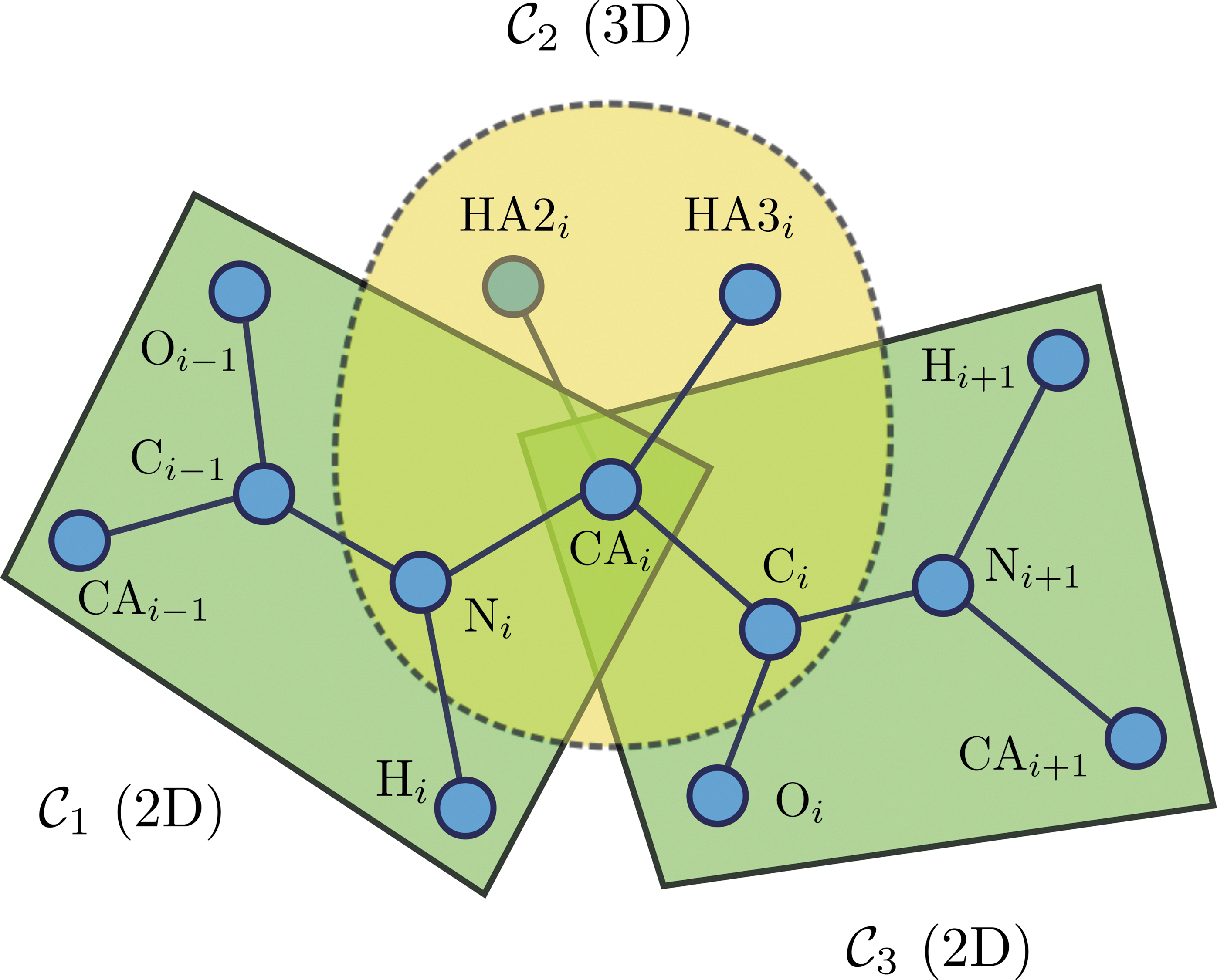
It can be observed that the protein contains many small intersecting cliques. For example, peptide planes, or aromatic rings, are two-dimensional (2D) cliques, and tetrahedral carbons form 3D cliques. As we show later, whenever there is a clique in the protein, the corresponding Gram matrix, K, can never be full-rank, which violates strict feasibility. By adapting and extending a technique called semidefinite facial reduction, not only do we obtain an equivalent problem that satisfies strict feasibility, but we also significantly reduce the SDP problem size.
2.3. Cliques in a protein molecule
A protein molecule with ℓ amino acid residues has ℓ + 1 planes in its backbone. Moreover, each amino acid has a different side chain with a different structure; therefore, the number of cliques in each side chain varies (see Appendix Tables 1 and 2 for the number of cliques in each amino acid side chain and other information about the cliques). We assume that the ith residue, ri, has si cliques in its side chain, denoted by \documentclass{aastex}\usepackage{amsbsy}\usepackage{amsfonts}\usepackage{amssymb}\usepackage{bm}\usepackage{mathrsfs}\usepackage{pifont}\usepackage{stmaryrd}\usepackage{textcomp}\usepackage{portland, xspace}\usepackage{amsmath, amsxtra}\pagestyle{empty}\DeclareMathSizes{10}{9}{7}{6}\begin{document}
$${\cal S}_i^{(1)} , \ldots , {\cal S}_i^{(s_i)}$$
\end{document}. For all amino acids (except glycine and proline), the first side chain clique is formed around the tetrahedral carbon CA, \documentclass{aastex}\usepackage{amsbsy}\usepackage{amsfonts}\usepackage{amssymb}\usepackage{bm}\usepackage{mathrsfs}\usepackage{pifont}\usepackage{stmaryrd}\usepackage{textcomp}\usepackage{portland, xspace}\usepackage{amsmath, amsxtra}\pagestyle{empty}\DeclareMathSizes{10}{9}{7}{6}\begin{document}
$${\cal S}_i^{(1)} = \{{\rm N}_i , {\rm CA}_i , {\rm HA}_i , {\rm CB}_i , {\rm C}_i \} $$
\end{document}, which intersects with two peptide planes \documentclass{aastex}\usepackage{amsbsy}\usepackage{amsfonts}\usepackage{amssymb}\usepackage{bm}\usepackage{mathrsfs}\usepackage{pifont}\usepackage{stmaryrd}\usepackage{textcomp}\usepackage{portland, xspace}\usepackage{amsmath, amsxtra}\pagestyle{empty}\DeclareMathSizes{10}{9}{7}{6}\begin{document}
$${\cal P}_{i - 1}$$
\end{document} and \documentclass{aastex}\usepackage{amsbsy}\usepackage{amsfonts}\usepackage{amssymb}\usepackage{bm}\usepackage{mathrsfs}\usepackage{pifont}\usepackage{stmaryrd}\usepackage{textcomp}\usepackage{portland, xspace}\usepackage{amsmath, amsxtra}\pagestyle{empty}\DeclareMathSizes{10}{9}{7}{6}\begin{document}
$${\cal P}_i$$
\end{document} in two atoms: \documentclass{aastex}\usepackage{amsbsy}\usepackage{amsfonts}\usepackage{amssymb}\usepackage{bm}\usepackage{mathrsfs}\usepackage{pifont}\usepackage{stmaryrd}\usepackage{textcomp}\usepackage{portland, xspace}\usepackage{amsmath, amsxtra}\pagestyle{empty}\DeclareMathSizes{10}{9}{7}{6}\begin{document}
$${\cal S}_i^{(1)} \cap {\cal P}_{i - 1} = \{{\rm N}_i , {\rm CA}_i \} $$
\end{document} and \documentclass{aastex}\usepackage{amsbsy}\usepackage{amsfonts}\usepackage{amssymb}\usepackage{bm}\usepackage{mathrsfs}\usepackage{pifont}\usepackage{stmaryrd}\usepackage{textcomp}\usepackage{portland, xspace}\usepackage{amsmath, amsxtra}\pagestyle{empty}\DeclareMathSizes{10}{9}{7}{6}\begin{document}
$${\cal S}_i^{(1)} \cap {\cal P}_{i} = \{{\rm CA}_i , {\rm C}_i \} $$
\end{document}. Side chain cliques for all twenty amino acids are listed in Appendix Table 2 (see Appendix B). There is a total of \documentclass{aastex}\usepackage{amsbsy}\usepackage{amsfonts}\usepackage{amssymb}\usepackage{bm}\usepackage{mathrsfs}\usepackage{pifont}\usepackage{stmaryrd}\usepackage{textcomp}\usepackage{portland, xspace}\usepackage{amsmath, amsxtra}\pagestyle{empty}\DeclareMathSizes{10}{9}{7}{6}\begin{document}
$$q = \ell + 1 + \sum\nolimits_{i = 1}^ \ell s_i$$
\end{document} cliques in the distance matrix of any protein. To simplify, let \documentclass{aastex}\usepackage{amsbsy}\usepackage{amsfonts}\usepackage{amssymb}\usepackage{bm}\usepackage{mathrsfs}\usepackage{pifont}\usepackage{stmaryrd}\usepackage{textcomp}\usepackage{portland, xspace}\usepackage{amsmath, amsxtra}\pagestyle{empty}\DeclareMathSizes{10}{9}{7}{6}\begin{document}
$${\cal C}_i = {\cal P}_{i - 1} , \ 1 \leq i \leq \ell + 1$$
\end{document}, and \documentclass{aastex}\usepackage{amsbsy}\usepackage{amsfonts}\usepackage{amssymb}\usepackage{bm}\usepackage{mathrsfs}\usepackage{pifont}\usepackage{stmaryrd}\usepackage{textcomp}\usepackage{portland, xspace}\usepackage{amsmath, amsxtra}\pagestyle{empty}\DeclareMathSizes{10}{9}{7}{6}\begin{document}
$${\cal C}_{\ell + 2} ={\cal S}_1^{(1)} , \ {\cal C}_{\ell + 2} = {\cal S}_1^{(2)} , \ldots , {\cal C}_{q} = {\cal S}_ \ell^{(s_ \ell)}$$
\end{document}. For properties of the cliques in the protein molecule, see Appendix A. See Figure 1 for an example with the Glycine amino acid as the i-th residue, together with its neighboring backbone planes.
The Glycine amino acid as the i-th residue, with its neighboring backbone planes.
2.4. Algorithm for finding the face of the structure
For t < n and \documentclass{aastex}\usepackage{amsbsy}\usepackage{amsfonts}\usepackage{amssymb}\usepackage{bm}\usepackage{mathrsfs}\usepackage{pifont}\usepackage{stmaryrd}\usepackage{textcomp}\usepackage{portland, xspace}\usepackage{amsmath, amsxtra}\pagestyle{empty}\DeclareMathSizes{10}{9}{7}{6}\begin{document}
$$U \in {\mathbb R}^{n \times t}$$
\end{document}, the set of matrices \documentclass{aastex}\usepackage{amsbsy}\usepackage{amsfonts}\usepackage{amssymb}\usepackage{bm}\usepackage{mathrsfs}\usepackage{pifont}\usepackage{stmaryrd}\usepackage{textcomp}\usepackage{portland, xspace}\usepackage{amsmath, amsxtra}\pagestyle{empty}\DeclareMathSizes{10}{9}{7}{6}\begin{document}
$$U {\cal S}^t_ {+} U^ \top$$
\end{document} is a face of \documentclass{aastex}\usepackage{amsbsy}\usepackage{amsfonts}\usepackage{amssymb}\usepackage{bm}\usepackage{mathrsfs}\usepackage{pifont}\usepackage{stmaryrd}\usepackage{textcomp}\usepackage{portland, xspace}\usepackage{amsmath, amsxtra}\pagestyle{empty}\DeclareMathSizes{10}{9}{7}{6}\begin{document}
$$S_ {+} ^n$$
\end{document} (in fact every face of \documentclass{aastex}\usepackage{amsbsy}\usepackage{amsfonts}\usepackage{amssymb}\usepackage{bm}\usepackage{mathrsfs}\usepackage{pifont}\usepackage{stmaryrd}\usepackage{textcomp}\usepackage{portland, xspace}\usepackage{amsmath, amsxtra}\pagestyle{empty}\DeclareMathSizes{10}{9}{7}{6}\begin{document}
$$S_ {+} ^n$$
\end{document} can be described in this way); see, e.g., Ramana et al. (1997). We let face (\documentclass{aastex}\usepackage{amsbsy}\usepackage{amsfonts}\usepackage{amssymb}\usepackage{bm}\usepackage{mathrsfs}\usepackage{pifont}\usepackage{stmaryrd}\usepackage{textcomp}\usepackage{portland, xspace}\usepackage{amsmath, amsxtra}\pagestyle{empty}\DeclareMathSizes{10}{9}{7}{6}\begin{document}
$${\cal F}$$
\end{document}) represent the smallest face containing a subset \documentclass{aastex}\usepackage{amsbsy}\usepackage{amsfonts}\usepackage{amssymb}\usepackage{bm}\usepackage{mathrsfs}\usepackage{pifont}\usepackage{stmaryrd}\usepackage{textcomp}\usepackage{portland, xspace}\usepackage{amsmath, amsxtra}\pagestyle{empty}\DeclareMathSizes{10}{9}{7}{6}\begin{document}
$${\cal F}$$
\end{document} of \documentclass{aastex}\usepackage{amsbsy}\usepackage{amsfonts}\usepackage{amssymb}\usepackage{bm}\usepackage{mathrsfs}\usepackage{pifont}\usepackage{stmaryrd}\usepackage{textcomp}\usepackage{portland, xspace}\usepackage{amsmath, amsxtra}\pagestyle{empty}\DeclareMathSizes{10}{9}{7}{6}\begin{document}
$$S_ {+} ^n$$
\end{document}; then we have the important property that \documentclass{aastex}\usepackage{amsbsy}\usepackage{amsfonts}\usepackage{amssymb}\usepackage{bm}\usepackage{mathrsfs}\usepackage{pifont}\usepackage{stmaryrd}\usepackage{textcomp}\usepackage{portland, xspace}\usepackage{amsmath, amsxtra}\pagestyle{empty}\DeclareMathSizes{10}{9}{7}{6}\begin{document}
$${\bf face} ({\cal F}) = U {\cal S}^t_ {+} U^ \top$$
\end{document} if and only if there exists \documentclass{aastex}\usepackage{amsbsy}\usepackage{amsfonts}\usepackage{amssymb}\usepackage{bm}\usepackage{mathrsfs}\usepackage{pifont}\usepackage{stmaryrd}\usepackage{textcomp}\usepackage{portland, xspace}\usepackage{amsmath, amsxtra}\pagestyle{empty}\DeclareMathSizes{10}{9}{7}{6}\begin{document}
$$Z \in {\cal S}^t_{+ +}$$
\end{document} such that \documentclass{aastex}\usepackage{amsbsy}\usepackage{amsfonts}\usepackage{amssymb}\usepackage{bm}\usepackage{mathrsfs}\usepackage{pifont}\usepackage{stmaryrd}\usepackage{textcomp}\usepackage{portland, xspace}\usepackage{amsmath, amsxtra}\pagestyle{empty}\DeclareMathSizes{10}{9}{7}{6}\begin{document}
$$UZU^ \top \in {\cal F}$$
\end{document}. Furthermore, in this case, we have that every \documentclass{aastex}\usepackage{amsbsy}\usepackage{amsfonts}\usepackage{amssymb}\usepackage{bm}\usepackage{mathrsfs}\usepackage{pifont}\usepackage{stmaryrd}\usepackage{textcomp}\usepackage{portland, xspace}\usepackage{amsmath, amsxtra}\pagestyle{empty}\DeclareMathSizes{10}{9}{7}{6}\begin{document}
$$Y \in {\cal F}$$
\end{document} can be decomposed as \documentclass{aastex}\usepackage{amsbsy}\usepackage{amsfonts}\usepackage{amssymb}\usepackage{bm}\usepackage{mathrsfs}\usepackage{pifont}\usepackage{stmaryrd}\usepackage{textcomp}\usepackage{portland, xspace}\usepackage{amsmath, amsxtra}\pagestyle{empty}\DeclareMathSizes{10}{9}{7}{6}\begin{document}
$$Y = UZU^ \top$$
\end{document}, for some \documentclass{aastex}\usepackage{amsbsy}\usepackage{amsfonts}\usepackage{amssymb}\usepackage{bm}\usepackage{mathrsfs}\usepackage{pifont}\usepackage{stmaryrd}\usepackage{textcomp}\usepackage{portland, xspace}\usepackage{amsmath, amsxtra}\pagestyle{empty}\DeclareMathSizes{10}{9}{7}{6}\begin{document}
$$Z \in {\cal S}_{+}^t$$
\end{document}, and the reduced feasible set \documentclass{aastex}\usepackage{amsbsy}\usepackage{amsfonts}\usepackage{amssymb}\usepackage{bm}\usepackage{mathrsfs}\usepackage{pifont}\usepackage{stmaryrd}\usepackage{textcomp}\usepackage{portland, xspace}\usepackage{amsmath, amsxtra}\pagestyle{empty}\DeclareMathSizes{10}{9}{7}{6}\begin{document}
$$\{Z \in {\cal S}_{+}^t : UZU^ \top \in {\cal F} \} $$
\end{document} has a strictly feasible point, giving us a problem that is more numerically stable to solve (problems that are not strictly feasible have a dual optimal set that is unbounded and therefore can be difficult to solve numerically; for more information, see Wei and Wolkowicz 2010). Moreover, if t ≪ n, this results in a significant reduction in the matrix size.
The Face of a Single Clique Here, we solve the Single Clique problem, which is defined as follows: Let D be a partial EDM of a protein. Suppose the first n1 points form a clique in the protein, such that for \documentclass{aastex}\usepackage{amsbsy}\usepackage{amsfonts}\usepackage{amssymb}\usepackage{bm}\usepackage{mathrsfs}\usepackage{pifont}\usepackage{stmaryrd}\usepackage{textcomp}\usepackage{portland, xspace}\usepackage{amsmath, amsxtra}\pagestyle{empty}\DeclareMathSizes{10}{9}{7}{6}\begin{document}
$${\cal C}_1 = \{1 , \ldots , n_1 \} $$
\end{document}, all distances are known. That is, the matrix \documentclass{aastex}\usepackage{amsbsy}\usepackage{amsfonts}\usepackage{amssymb}\usepackage{bm}\usepackage{mathrsfs}\usepackage{pifont}\usepackage{stmaryrd}\usepackage{textcomp}\usepackage{portland, xspace}\usepackage{amsmath, amsxtra}\pagestyle{empty}\DeclareMathSizes{10}{9}{7}{6}\begin{document}
$$D_1 = D [{\cal C}_1]$$
\end{document} is completely specified. Moreover, let r1 = embdim(D1). We now show how to compute the smallest face containing the feasible set \documentclass{aastex}\usepackage{amsbsy}\usepackage{amsfonts}\usepackage{amssymb}\usepackage{bm}\usepackage{mathrsfs}\usepackage{pifont}\usepackage{stmaryrd}\usepackage{textcomp}\usepackage{portland, xspace}\usepackage{amsmath, amsxtra}\pagestyle{empty}\DeclareMathSizes{10}{9}{7}{6}\begin{document}
$$\{K \in {\cal S}_ {+} ^n: {\rm K} (K [{\cal C}_1]) = D_1 \} $$
\end{document}.
Theorem 2
(Single Clique, Krislock and Wolkowicz, 2010). Let the matrix\documentclass{aastex}\usepackage{amsbsy}\usepackage{amsfonts}\usepackage{amssymb}\usepackage{bm}\usepackage{mathrsfs}\usepackage{pifont}\usepackage{stmaryrd}\usepackage{textcomp}\usepackage{portland, xspace}\usepackage{amsmath, amsxtra}\pagestyle{empty}\DeclareMathSizes{10}{9}{7}{6}\begin{document}
$$U \in {\mathbb R}^{n \times (n - n_1 + r_1 + 1)}$$
\end{document}be defined as follows:
Then U1 has full column rank,1\documentclass{aastex}\usepackage{amsbsy}\usepackage{amsfonts}\usepackage{amssymb}\usepackage{bm}\usepackage{mathrsfs}\usepackage{pifont}\usepackage{stmaryrd}\usepackage{textcomp}\usepackage{portland, xspace}\usepackage{amsmath, amsxtra}\pagestyle{empty}\DeclareMathSizes{10}{9}{7}{6}\begin{document}
$${\in}$$
\end{document}range(U), and\documentclass{aastex}\usepackage{amsbsy}\usepackage{amsfonts}\usepackage{amssymb}\usepackage{bm}\usepackage{mathrsfs}\usepackage{pifont}\usepackage{stmaryrd}\usepackage{textcomp}\usepackage{portland, xspace}\usepackage{amsmath, amsxtra}\pagestyle{empty}\DeclareMathSizes{10}{9}{7}{6}\begin{document}
\begin{align*}{\bf face} \{K \in {\cal S}^n_ {+} : {\rm K} (
K [{\cal C}_1]) = D [{\cal C}_1] \} = U_1{\cal S}_ {+} ^{n
- n_1 + r_1 + 1}U_1^ \top.\end{align*}
\end{document}
Computing the V1 Matrix In Theorem 2, we can find V1 by computing the eigen decomposition of K†(D[C1]) as follows:
\documentclass{aastex}\usepackage{amsbsy}\usepackage{amsfonts}\usepackage{amssymb}\usepackage{bm}\usepackage{mathrsfs}\usepackage{pifont}\usepackage{stmaryrd}\usepackage{textcomp}\usepackage{portland, xspace}\usepackage{amsmath, amsxtra}\pagestyle{empty}\DeclareMathSizes{10}{9}{7}{6}\begin{document}
\begin{align*}{\rm K}^{\dag} (D [{\cal C}_1]) = V_1 \Lambda_1 V_1^ \top , \quad V_1 \in {\mathbb R}^{{n_1} \times {r_1}} , \ \Lambda_1 \in {\cal S}_{+ +}^{r_1}. \tag{6}\end{align*}
\end{document}
It can be seen that V1 has full column rank (columns are orthonormal) and also that range(V1) = range(K†(D1)).
2.5. The face of a protein molecule
The protein molecule is made of q cliques, \documentclass{aastex}\usepackage{amsbsy}\usepackage{amsfonts}\usepackage{amssymb}\usepackage{bm}\usepackage{mathrsfs}\usepackage{pifont}\usepackage{stmaryrd}\usepackage{textcomp}\usepackage{portland, xspace}\usepackage{amsmath, amsxtra}\pagestyle{empty}\DeclareMathSizes{10}{9}{7}{6}\begin{document}
$$\{{\cal C}_1 , \ldots , {\cal C}_q \} $$
\end{document}, such that D[Cl] is known, and we have rl = embdim(D[Cl]), and nl = |Cl|. Let \documentclass{aastex}\usepackage{amsbsy}\usepackage{amsfonts}\usepackage{amssymb}\usepackage{bm}\usepackage{mathrsfs}\usepackage{pifont}\usepackage{stmaryrd}\usepackage{textcomp}\usepackage{portland, xspace}\usepackage{amsmath, amsxtra}\pagestyle{empty}\DeclareMathSizes{10}{9}{7}{6}\begin{document}
$${\cal F}$$
\end{document} be the feasible set of the SDP problem. If for each clique \documentclass{aastex}\usepackage{amsbsy}\usepackage{amsfonts}\usepackage{amssymb}\usepackage{bm}\usepackage{mathrsfs}\usepackage{pifont}\usepackage{stmaryrd}\usepackage{textcomp}\usepackage{portland, xspace}\usepackage{amsmath, amsxtra}\pagestyle{empty}\DeclareMathSizes{10}{9}{7}{6}\begin{document}
$${\cal C}_l$$
\end{document}, we define \documentclass{aastex}\usepackage{amsbsy}\usepackage{amsfonts}\usepackage{amssymb}\usepackage{bm}\usepackage{mathrsfs}\usepackage{pifont}\usepackage{stmaryrd}\usepackage{textcomp}\usepackage{portland, xspace}\usepackage{amsmath, amsxtra}\pagestyle{empty}\DeclareMathSizes{10}{9}{7}{6}\begin{document}
$${\cal F}_l : = \{K \in {\cal S}^n_ {+} : {\rm K} (K [{\cal
C}_l]) = D [{\cal C}_l] \} $$
\end{document}, then
\documentclass{aastex}\usepackage{amsbsy}\usepackage{amsfonts}\usepackage{amssymb}\usepackage{bm}\usepackage{mathrsfs}\usepackage{pifont}\usepackage{stmaryrd}\usepackage{textcomp}\usepackage{portland, xspace}\usepackage{amsmath, amsxtra}\pagestyle{empty}\DeclareMathSizes{10}{9}{7}{6}\begin{document}
\begin{align*}{\cal F} \subseteq \left(\bigcap_{l = 1}^q {\cal
F}_l \right) \cap {\cal S}^n_C , \tag{7}\end{align*}
\end{document}
where \documentclass{aastex}\usepackage{amsbsy}\usepackage{amsfonts}\usepackage{amssymb}\usepackage{bm}\usepackage{mathrsfs}\usepackage{pifont}\usepackage{stmaryrd}\usepackage{textcomp}\usepackage{portland, xspace}\usepackage{amsmath, amsxtra}\pagestyle{empty}\DeclareMathSizes{10}{9}{7}{6}\begin{document}
$${\cal S}^n_C : = \{K \in {\cal S}^n : K {\bf 1} = {\bf 0} \}
$$
\end{document} are the centered symmetric matrices. For \documentclass{aastex}\usepackage{amsbsy}\usepackage{amsfonts}\usepackage{amssymb}\usepackage{bm}\usepackage{mathrsfs}\usepackage{pifont}\usepackage{stmaryrd}\usepackage{textcomp}\usepackage{portland, xspace}\usepackage{amsmath, amsxtra}\pagestyle{empty}\DeclareMathSizes{10}{9}{7}{6}\begin{document}
$$l = 1 , \ldots , q$$
\end{document}, let \documentclass{aastex}\usepackage{amsbsy}\usepackage{amsfonts}\usepackage{amssymb}\usepackage{bm}\usepackage{mathrsfs}\usepackage{pifont}\usepackage{stmaryrd}\usepackage{textcomp}\usepackage{portland, xspace}\usepackage{amsmath, amsxtra}\pagestyle{empty}\DeclareMathSizes{10}{9}{7}{6}\begin{document}
$$F_l : =\, {\bf face} ({\cal F}_l) = U_l {\cal S}_ {+} ^{n -
n_l + r_l + 1}U_l^ \top$$
\end{document}, where Ul is computed as in Theorem 2. We have (Krislock and Wolkowicz, 2010):
\documentclass{aastex}\usepackage{amsbsy}\usepackage{amsfonts}\usepackage{amssymb}\usepackage{bm}\usepackage{mathrsfs}\usepackage{pifont}\usepackage{stmaryrd}\usepackage{textcomp}\usepackage{portland, xspace}\usepackage{amsmath, amsxtra}\pagestyle{empty}\DeclareMathSizes{10}{9}{7}{6}\begin{document}
\begin{align*}\left(\bigcap_{l = 1}^q {\cal F}_l \right) \cap {
\cal S}^n_C \subseteq \left(\bigcap_{l = 1}^q U_l {\cal S}_ {+}
^{n - n_l + r_l + 1}U_l^ \top \right) \cap {\cal S}^n_C = (U {
\cal S}_ {+} ^{k} U^ \top) \cap {\cal S}^n_C ,
\tag{8}\end{align*}
\end{document}
where \documentclass{aastex}\usepackage{amsbsy}\usepackage{amsfonts}\usepackage{amssymb}\usepackage{bm}\usepackage{mathrsfs}\usepackage{pifont}\usepackage{stmaryrd}\usepackage{textcomp}\usepackage{portland, xspace}\usepackage{amsmath, amsxtra}\pagestyle{empty}\DeclareMathSizes{10}{9}{7}{6}\begin{document}
$$U \in {\mathbb R}^{n \times k}$$
\end{document} is a full column rank matrix that satisfies range\documentclass{aastex}\usepackage{amsbsy}\usepackage{amsfonts}\usepackage{amssymb}\usepackage{bm}\usepackage{mathrsfs}\usepackage{pifont}\usepackage{stmaryrd}\usepackage{textcomp}\usepackage{portland, xspace}\usepackage{amsmath, amsxtra}\pagestyle{empty}\DeclareMathSizes{10}{9}{7}{6}\begin{document}
$$(U) = \bigcap\nolimits_{l = 1}^q {\bf range} (U_l)$$
\end{document}.
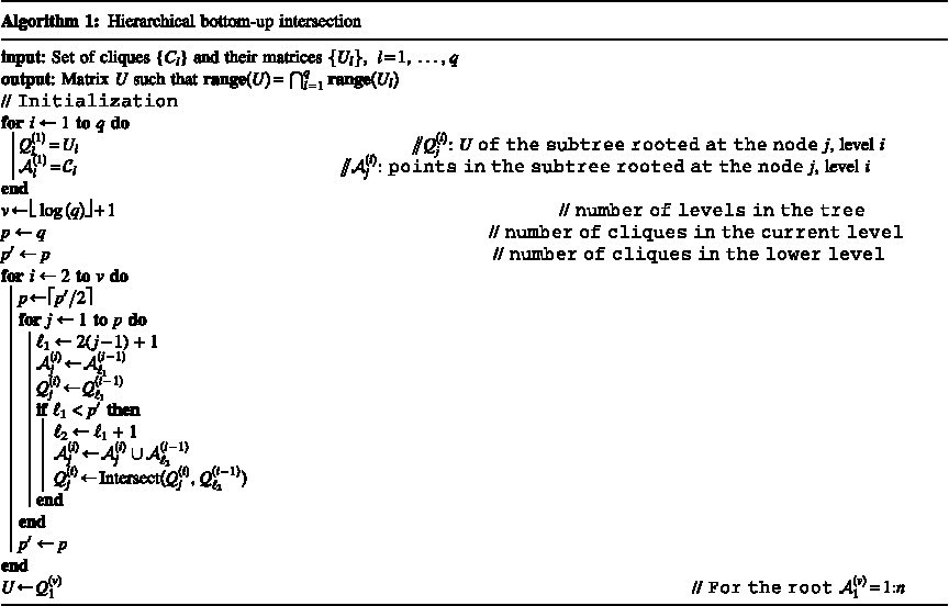
We now have an efficient method for computing the face of the feasible set \documentclass{aastex}\usepackage{amsbsy}\usepackage{amsfonts}\usepackage{amssymb}\usepackage{bm}\usepackage{mathrsfs}\usepackage{pifont}\usepackage{stmaryrd}\usepackage{textcomp}\usepackage{portland, xspace}\usepackage{amsmath, amsxtra}\pagestyle{empty}\DeclareMathSizes{10}{9}{7}{6}\begin{document}
$${\cal F}$$
\end{document}. To have better numerical accuracy, we developed a bottom-up algorithm for intersecting subspaces (see Algorithm 1 in the Appendix).
After computing U, we can decompose the Gram matrix as \documentclass{aastex}\usepackage{amsbsy}\usepackage{amsfonts}\usepackage{amssymb}\usepackage{bm}\usepackage{mathrsfs}\usepackage{pifont}\usepackage{stmaryrd}\usepackage{textcomp}\usepackage{portland, xspace}\usepackage{amsmath, amsxtra}\pagestyle{empty}\DeclareMathSizes{10}{9}{7}{6}\begin{document}
$$K = UZU^ \top$$
\end{document}, for \documentclass{aastex}\usepackage{amsbsy}\usepackage{amsfonts}\usepackage{amssymb}\usepackage{bm}\usepackage{mathrsfs}\usepackage{pifont}\usepackage{stmaryrd}\usepackage{textcomp}\usepackage{portland, xspace}\usepackage{amsmath, amsxtra}\pagestyle{empty}\DeclareMathSizes{10}{9}{7}{6}\begin{document}
$$Z \in {\cal S}^k_ {+}$$
\end{document}. However, by exploiting the centering constraint, K1 = 0, we can reduce the matrix size one more. If \documentclass{aastex}\usepackage{amsbsy}\usepackage{amsfonts}\usepackage{amssymb}\usepackage{bm}\usepackage{mathrsfs}\usepackage{pifont}\usepackage{stmaryrd}\usepackage{textcomp}\usepackage{portland, xspace}\usepackage{amsmath, amsxtra}\pagestyle{empty}\DeclareMathSizes{10}{9}{7}{6}\begin{document}
$$V \in {\mathbb R}^{k \times (k - 1)}$$
\end{document} has full column rank and satisfies range(V) = null\documentclass{aastex}\usepackage{amsbsy}\usepackage{amsfonts}\usepackage{amssymb}\usepackage{bm}\usepackage{mathrsfs}\usepackage{pifont}\usepackage{stmaryrd}\usepackage{textcomp}\usepackage{portland, xspace}\usepackage{amsmath, amsxtra}\pagestyle{empty}\DeclareMathSizes{10}{9}{7}{6}\begin{document}
$$({\bf 1}^ \top U)$$
\end{document}, then we have (Krislock and Wolkowicz, 2010):
\documentclass{aastex}\usepackage{amsbsy}\usepackage{amsfonts}\usepackage{amssymb}\usepackage{bm}\usepackage{mathrsfs}\usepackage{pifont}\usepackage{stmaryrd}\usepackage{textcomp}\usepackage{portland, xspace}\usepackage{amsmath, amsxtra}\pagestyle{empty}\DeclareMathSizes{10}{9}{7}{6}\begin{document}
\begin{align*}{\cal F} \subseteq (UV) {\cal S}_ {+} ^{k - 1}
(UV) ^ \top. \tag{9}\end{align*}
\end{document}
For more details on facial reduction for Euclidean distance matrix completion problems, see Krislock (2010).
Constraints for Preserving the Structure of Cliques If we find a base set of points \documentclass{aastex}\usepackage{amsbsy}\usepackage{amsfonts}\usepackage{amssymb}\usepackage{bm}\usepackage{mathrsfs}\usepackage{pifont}\usepackage{stmaryrd}\usepackage{textcomp}\usepackage{portland, xspace}\usepackage{amsmath, amsxtra}\pagestyle{empty}\DeclareMathSizes{10}{9}{7}{6}\begin{document}
$${\cal B}_l$$
\end{document} in each clique \documentclass{aastex}\usepackage{amsbsy}\usepackage{amsfonts}\usepackage{amssymb}\usepackage{bm}\usepackage{mathrsfs}\usepackage{pifont}\usepackage{stmaryrd}\usepackage{textcomp}\usepackage{portland, xspace}\usepackage{amsmath, amsxtra}\pagestyle{empty}\DeclareMathSizes{10}{9}{7}{6}\begin{document}
$${\cal C}_l$$
\end{document} such that embdim\documentclass{aastex}\usepackage{amsbsy}\usepackage{amsfonts}\usepackage{amssymb}\usepackage{bm}\usepackage{mathrsfs}\usepackage{pifont}\usepackage{stmaryrd}\usepackage{textcomp}\usepackage{portland, xspace}\usepackage{amsmath, amsxtra}\pagestyle{empty}\DeclareMathSizes{10}{9}{7}{6}\begin{document}
$$(D [{\cal B}_l])= r_l$$
\end{document}, then by fixing the distances between points in the base set and fixing the distances between points in \documentclass{aastex}\usepackage{amsbsy}\usepackage{amsfonts}\usepackage{amssymb}\usepackage{bm}\usepackage{mathrsfs}\usepackage{pifont}\usepackage{stmaryrd}\usepackage{textcomp}\usepackage{portland, xspace}\usepackage{amsmath, amsxtra}\pagestyle{empty}\DeclareMathSizes{10}{9}{7}{6}\begin{document}
$${\cal C}_l \backslash {\cal B}_l$$
\end{document} and points in \documentclass{aastex}\usepackage{amsbsy}\usepackage{amsfonts}\usepackage{amssymb}\usepackage{bm}\usepackage{mathrsfs}\usepackage{pifont}\usepackage{stmaryrd}\usepackage{textcomp}\usepackage{portland, xspace}\usepackage{amsmath, amsxtra}\pagestyle{empty}\DeclareMathSizes{10}{9}{7}{6}\begin{document}
$${\cal B}_l$$
\end{document}, the entire clique is kept rigid. Therefore, we need to fix only the distances between base points (Alipanahi et al., 2012), resulting in a three- to four-fold reduction in the number of equality constraints. We call the reduced set of equality constraints \documentclass{aastex}\usepackage{amsbsy}\usepackage{amsfonts}\usepackage{amssymb}\usepackage{bm}\usepackage{mathrsfs}\usepackage{pifont}\usepackage{stmaryrd}\usepackage{textcomp}\usepackage{portland, xspace}\usepackage{amsmath, amsxtra}\pagestyle{empty}\DeclareMathSizes{10}{9}{7}{6}\begin{document}
$${\cal E}_{{\rm FR}}$$
\end{document}.
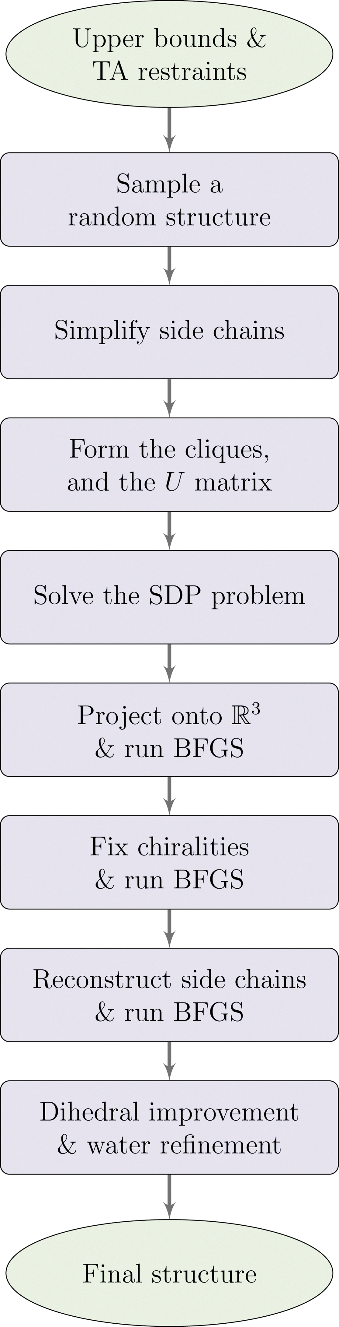
2.6. Solving and refining the reduced SDP problem
The SPROS method flowchart is depicted in Appendix Figure 3. In it, we describe the blocks for solving the SDP problem and for refining the solution. From Equation (9), we can formulate the reduced SDP problem as follows:
\documentclass{aastex}\usepackage{amsbsy}\usepackage{amsfonts}\usepackage{amssymb}\usepackage{bm}\usepackage{mathrsfs}\usepackage{pifont}\usepackage{stmaryrd}\usepackage{textcomp}\usepackage{portland, xspace}\usepackage{amsmath, amsxtra}\pagestyle{empty}\DeclareMathSizes{10}{9}{7}{6}\begin{document}
\begin{align*}
{\rm minimize} \quad \gamma & \langle I , Z \rangle + \sum
\limits_{ij} w_{ij} \xi_{ij} + \sum \limits_{ij} w^{\prime}_{ij}
\zeta_{ij} \tag{10}\end{align*}
\end{document}\documentclass{aastex}\usepackage{amsbsy}\usepackage{amsfonts}\usepackage{amssymb}\usepackage{bm}\usepackage{mathrsfs}\usepackage{pifont}\usepackage{stmaryrd}\usepackage{textcomp}\usepackage{portland, xspace}\usepackage{amsmath, amsxtra}\pagestyle{empty}\DeclareMathSizes{10}{9}{7}{6}\begin{document}
\begin{align*}{\rm subject \ to} \quad & \langle A^{
\prime}_{ij} , Z \rangle = e_{ij} , \ (i , j) \in {\cal E}_{
\rm FR} \\\qquad\qquad\quad & \langle A^{\prime}_{ij} , Z \rangle
\leq u_{ij} + \xi_{ij} , \ (i , j) \in {\cal U}
\\\qquad\qquad\quad & \langle A^{\prime}_{ij} , Z \rangle \geq
l_{ij} - \zeta_{ij} , \ (i , j) \in {\cal L} \\
\qquad\qquad\quad& \xi_{ij} \in {\mathbb R}_ {+} , \ (i , j) \in
{\cal U} , \quad \zeta_{ij} \in {\mathbb R}_ {+} , \ (i , j)
\in {\cal L} \\\qquad\qquad\quad & Z \in {\cal S}^{k - 1}_ {+} ,
\end{align*}
\end{document}
Weights and the regularization parameter For each type of upper and lower bound, we define a fixed penalizing weight for violations. For example, for upper bounds (similarly for lower bounds) we have \documentclass{aastex}\usepackage{amsbsy}\usepackage{amsfonts}\usepackage{amssymb}\usepackage{bm}\usepackage{mathrsfs}\usepackage{pifont}\usepackage{stmaryrd}\usepackage{textcomp}\usepackage{portland, xspace}\usepackage{amsmath, amsxtra}\pagestyle{empty}\DeclareMathSizes{10}{9}{7}{6}\begin{document}
$$\forall (i , j) \ \in {\cal U}_{\cal X} , w_{ij} = w_{\cal X}$$
\end{document}. We set \documentclass{aastex}\usepackage{amsbsy}\usepackage{amsfonts}\usepackage{amssymb}\usepackage{bm}\usepackage{mathrsfs}\usepackage{pifont}\usepackage{stmaryrd}\usepackage{textcomp}\usepackage{portland, xspace}\usepackage{amsmath, amsxtra}\pagestyle{empty}\DeclareMathSizes{10}{9}{7}{6}\begin{document}
$$w_{\cal N} = 1$$
\end{document} and \documentclass{aastex}\usepackage{amsbsy}\usepackage{amsfonts}\usepackage{amssymb}\usepackage{bm}\usepackage{mathrsfs}\usepackage{pifont}\usepackage{stmaryrd}\usepackage{textcomp}\usepackage{portland, xspace}\usepackage{amsmath, amsxtra}\pagestyle{empty}\DeclareMathSizes{10}{9}{7}{6}\begin{document}
$$w_{\cal H} = w_{\cal D} = w_{\cal T} = 10$$
\end{document} because upper bounds from hydrogen bonds and disulfide/salt bridges are assumed to be more accurate than are NOE-derived upper bounds. Moreover, the range of torsion angle violations is 10 times smaller than NOE violations.
Let \documentclass{aastex}\usepackage{amsbsy}\usepackage{amsfonts}\usepackage{amssymb}\usepackage{bm}\usepackage{mathrsfs}\usepackage{pifont}\usepackage{stmaryrd}\usepackage{textcomp}\usepackage{portland, xspace}\usepackage{amsmath, amsxtra}\pagestyle{empty}\DeclareMathSizes{10}{9}{7}{6}\begin{document}
$$m_{\cal U} = \mid {\cal U} \mid$$
\end{document} and R be the radius of the protein. Then, the maximum upper bound violation is 2R. Moreover, \documentclass{aastex}\usepackage{amsbsy}\usepackage{amsfonts}\usepackage{amssymb}\usepackage{bm}\usepackage{mathrsfs}\usepackage{pifont}\usepackage{stmaryrd}\usepackage{textcomp}\usepackage{portland, xspace}\usepackage{amsmath, amsxtra}\pagestyle{empty}\DeclareMathSizes{10}{9}{7}{6}\begin{document}
$$\langle I , Z \rangle \leq nR$$
\end{document}. Discarding the role of lower bound violations, with the goal of approximately balancing the two terms, a suitable γ is:
\documentclass{aastex}\usepackage{amsbsy}\usepackage{amsfonts}\usepackage{amssymb}\usepackage{bm}\usepackage{mathrsfs}\usepackage{pifont}\usepackage{stmaryrd}\usepackage{textcomp}\usepackage{portland, xspace}\usepackage{amsmath, amsxtra}\pagestyle{empty}\DeclareMathSizes{10}{9}{7}{6}\begin{document}
\begin{align*}\gamma n R \approx 2 \varepsilon w m_ {\cal U} R
\quad \Rightarrow \quad \gamma = \frac {2 \varepsilon w m_ {\cal
U}} {n} , \tag {11} \end{align*}
\end{document}
where 0 ≤ ɛ ≤ 1 is the fraction of violated upper bounds. In practice ɛ ≈ 0.01 – 0.30 and \documentclass{aastex}\usepackage{amsbsy}\usepackage{amsfonts}\usepackage{amssymb}\usepackage{bm}\usepackage{mathrsfs}\usepackage{pifont}\usepackage{stmaryrd}\usepackage{textcomp}\usepackage{portland, xspace}\usepackage{amsmath, amsxtra}\pagestyle{empty}\DeclareMathSizes{10}{9}{7}{6}\begin{document}
$${\bar \gamma} \approx wm_{\cal U} / {50 n}$$
\end{document} works well.
Post-Processing We perform a refinement on the raw structure determined by the SDP solver. For this refinement, we use a BFGS-based quasi-Newton method (Lewis and Overton, 2012) that only requires the value of the objective function and its gradient at each point. Letting X(0) = XSDP, we iteratively minimize the following objective function:
\documentclass{aastex}\usepackage{amsbsy}\usepackage{amsfonts}\usepackage{amssymb}\usepackage{bm}\usepackage{mathrsfs}\usepackage{pifont}\usepackage{stmaryrd}\usepackage{textcomp}\usepackage{portland, xspace}\usepackage{amsmath, amsxtra}\pagestyle{empty}\DeclareMathSizes{10}{9}{7}{6}\begin{document}
\begin{align*}
{\phi (X)} = &w_{\cal E} \sum\limits_{(i , j) \in {\cal
E}} \left(\parallel \textbf{\textit{x}}_i - \textbf{\textit{x}}_j
\parallel - e_{ij} \right) ^2 + w_{\cal U} \sum\limits_{(i ,
j) \in {\cal U}} f \left(\parallel \textbf{\textit{x}}_i -
\textbf{\textit{x}}_j \parallel - u_{ij} \right) ^2 \\ & + w_{
\cal L} \sum\limits_{(i , j) \in {\cal L}} g \left(
\parallel \textbf{\textit{x}}_i - \textbf{\textit{x}}_j \parallel
- l_{ij} \right) ^2 + w_{\cal R} \sum\limits_{i = 1}^{n}
\parallel \textbf{\textit{x}}_i
\parallel ^2 , \tag{12}\end{align*}
\end{document}
where f (θ) = max(0,θ) and g(θ) = min(0,−θ). We set wɛ = 2, \documentclass{aastex}\usepackage{amsbsy}\usepackage{amsfonts}\usepackage{amssymb}\usepackage{bm}\usepackage{mathrsfs}\usepackage{pifont}\usepackage{stmaryrd}\usepackage{textcomp}\usepackage{portland, xspace}\usepackage{amsmath, amsxtra}\pagestyle{empty}\DeclareMathSizes{10}{9}{7}{6}\begin{document}
$$w_{\cal U}$$
\end{document} = 1, and \documentclass{aastex}\usepackage{amsbsy}\usepackage{amsfonts}\usepackage{amssymb}\usepackage{bm}\usepackage{mathrsfs}\usepackage{pifont}\usepackage{stmaryrd}\usepackage{textcomp}\usepackage{portland, xspace}\usepackage{amsmath, amsxtra}\pagestyle{empty}\DeclareMathSizes{10}{9}{7}{6}\begin{document}
$$w_{\cal L} = 1$$
\end{document}. In addition, to balance the regularization term, we set
\documentclass{aastex}\usepackage{amsbsy}\usepackage{amsfonts}\usepackage{amssymb}\usepackage{bm}\usepackage{mathrsfs}\usepackage{pifont}\usepackage{stmaryrd}\usepackage{textcomp}\usepackage{portland, xspace}\usepackage{amsmath, amsxtra}\pagestyle{empty}\DeclareMathSizes{10}{9}{7}{6}\begin{document}
\begin{align*}w_ {\cal R} = \alpha \frac {\phi (X^ {(0)}
) \mid _ {w_R = 0}} {25 \sum\nolimits_ {i = 1} ^ {n}
\parallel \textbf {\textit {x}}^{(0)}_i \parallel ^2
} ,\end{align*}
\end{document}
where −1 ≤ α ≤ 1 is a parameter controlling the regularization. If α < 0, the distances between atoms are maximized, because, after projection, some of the distances have been shortened, this term helps to compensate for that error. However, if α > 0, the distances between atoms are minimized, resulting in better packing of atoms in the protein molecule. In practice, different values for α can be used to generate slightly different structures, thus creating a bundle of structures.
Fixing incorrect chiralities Chirality constraints cannot be enforced using only distances. Consequently, some chiral centers may have the incorrect enantiomer. In this step, SPROS checks the chiral centers and resolves any problems.
Improving the stereochemical quality Williamson and Craven (2009) have described the effectiveness of explicit solvent refinement of NMR structures and suggest that it should be a standard procedure. For protein structures that have regions of high mobility/uncertainty due to few or no NOE observations, we have successfully employed a hybrid protocol from XPLOR-NIH that incorporates thin-layer water refinement (Linge et al., 2003) and a multidimensional torsion angle database (Kuszewski et al., 1996, 1997).
3. Results
We tested the performance of SPROS on 18 proteins: 15 protein data sets from the database of converted restraints (DOCR) database in the NMR restraints grid (Doreleijers et al., 2003, 2005) and three protein data sets from Donaldson's laboratory at York University, Toronto, Canada. We chose proteins with different sizes and topologies, as listed in Table 1. Finally, the input to the SPROS method is exactly the same as the input to the widely used CYANA method.
Information About the Proteins Used in Testing SPROS
The second, third, and fourth columns list the topologies, sequence lengths, and molecular weight of the proteins; the fifth and sixth columns, n and n′, list the original and reduced SDP matrix sizes, respectively. The seventh column lists the number of cliques in the protein. The eighth and ninth columns, \documentclass{aastex}\usepackage{amsbsy}\usepackage{amsfonts}\usepackage{amssymb}\usepackage{bm}\usepackage{mathrsfs}\usepackage{pifont}\usepackage{stmaryrd}\usepackage{textcomp}\usepackage{portland, xspace}\usepackage{amsmath, amsxtra}\pagestyle{empty}\DeclareMathSizes{10}{9}{7}{6}\begin{document}
$$m_{\cal E}$$
\end{document} and \documentclass{aastex}\usepackage{amsbsy}\usepackage{amsfonts}\usepackage{amssymb}\usepackage{bm}\usepackage{mathrsfs}\usepackage{pifont}\usepackage{stmaryrd}\usepackage{textcomp}\usepackage{portland, xspace}\usepackage{amsmath, amsxtra}\pagestyle{empty}\DeclareMathSizes{10}{9}{7}{6}\begin{document}
$$m^{\prime}_{\cal E}$$
\end{document}, list the number of equality constraints in the original and reduced problems, respectively. The 10th column, \documentclass{aastex}\usepackage{amsbsy}\usepackage{amsfonts}\usepackage{amssymb}\usepackage{bm}\usepackage{mathrsfs}\usepackage{pifont}\usepackage{stmaryrd}\usepackage{textcomp}\usepackage{portland, xspace}\usepackage{amsmath, amsxtra}\pagestyle{empty}\DeclareMathSizes{10}{9}{7}{6}\begin{document}
$$m_{\cal U}$$
\end{document}, lists the total number of upper bounds for each protein. The 11th column, bound types, lists intra-residue, |i − j| = 0, sequential, |i − j| = 1, medium range, 1 < |i − j| ≤ 4, and long range, |i − j| > 4, respectively, in percentile. The 12th column, \documentclass{aastex}\usepackage{amsbsy}\usepackage{amsfonts}\usepackage{amssymb}\usepackage{bm}\usepackage{mathrsfs}\usepackage{pifont}\usepackage{stmaryrd}\usepackage{textcomp}\usepackage{portland, xspace}\usepackage{amsmath, amsxtra}\pagestyle{empty}\DeclareMathSizes{10}{9}{7}{6}\begin{document}
$$\bar{m}_{\cal U} \pm s_{\cal U}$$
\end{document}, lists the average number of upper bounds per residue, together with the standard deviation. The 13th column, \documentclass{aastex}\usepackage{amsbsy}\usepackage{amsfonts}\usepackage{amssymb}\usepackage{bm}\usepackage{mathrsfs}\usepackage{pifont}\usepackage{stmaryrd}\usepackage{textcomp}\usepackage{portland, xspace}\usepackage{amsmath, amsxtra}\pagestyle{empty}\DeclareMathSizes{10}{9}{7}{6}\begin{document}
$$m_{\cal N}$$
\end{document}, lists the number of NOE-inferred upper bounds. The 14th column, \documentclass{aastex}\usepackage{amsbsy}\usepackage{amsfonts}\usepackage{amssymb}\usepackage{bm}\usepackage{mathrsfs}\usepackage{pifont}\usepackage{stmaryrd}\usepackage{textcomp}\usepackage{portland, xspace}\usepackage{amsmath, amsxtra}\pagestyle{empty}\DeclareMathSizes{10}{9}{7}{6}\begin{document}
$$p_{\cal U}$$
\end{document}, lists the fraction of pseudo-atoms in the upper bounds in percentile. The last two columns, \documentclass{aastex}\usepackage{amsbsy}\usepackage{amsfonts}\usepackage{amssymb}\usepackage{bm}\usepackage{mathrsfs}\usepackage{pifont}\usepackage{stmaryrd}\usepackage{textcomp}\usepackage{portland, xspace}\usepackage{amsmath, amsxtra}\pagestyle{empty}\DeclareMathSizes{10}{9}{7}{6}\begin{document}
$$m_{\cal T}$$
\end{document} and \documentclass{aastex}\usepackage{amsbsy}\usepackage{amsfonts}\usepackage{amssymb}\usepackage{bm}\usepackage{mathrsfs}\usepackage{pifont}\usepackage{stmaryrd}\usepackage{textcomp}\usepackage{portland, xspace}\usepackage{amsmath, amsxtra}\pagestyle{empty}\DeclareMathSizes{10}{9}{7}{6}\begin{document}
$$m_{\cal H}$$
\end{document}, list the number of upper bounds inferred from torsion angle restraints, and hydrogen bonds, disulfide and salt bridges, respectively.
3.1. Implementation
The SPROS method has been implemented and tested in Matlab 7.13 (apart from the water refinement, which is done by XPLOR-NIH). For solving the SDP problem, we used the SDPT3 method (Tütüncü et al., 2003). For minimizing the post-processing objective function (Eq. 12), we used the BFGS-based quasi-Newton method implementation by Lewis and Overton (2012). All the experiments were carried out on an Ubuntu 11.04 Linux PC with a 2.8 GHz Intel Core i7 Quad-Core processor and 8 GB of memory.
3.2. Determined structures
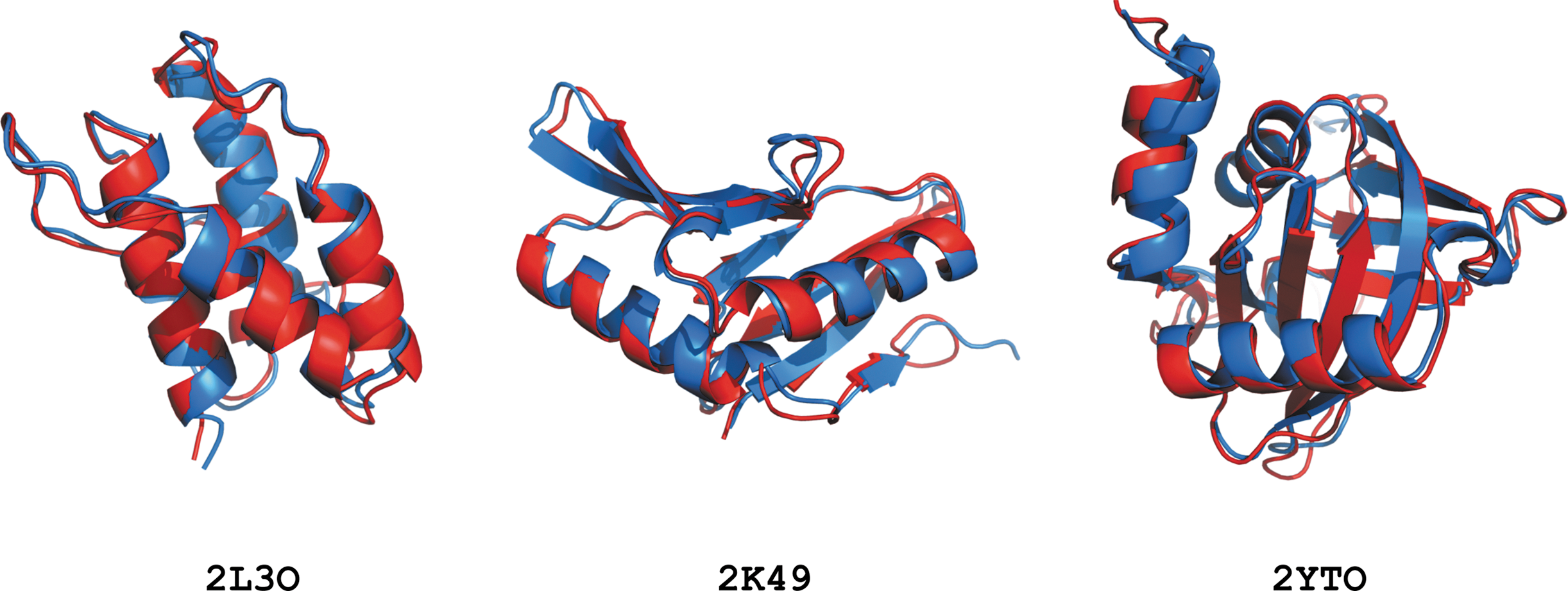
From the 18 test proteins, 9 of them were calculated with backbone RMSDs less than or equal to 1.0Å, and 16 have backbone RMSDs less than 1.5Å. Detailed analysis of calculated structures is listed in Table 2. The superimposition of the SPROS and reference structures for three of the proteins are depicted in Figure 2. More detailed information about the determined structures can be found in Alipanahi, (2011).
Superimposition of structures determined by SPROS in blue and the reference structures in red.
Information About Determined Structures of the Test Proteins
RMSD
Violations
Ramachandran
ID
ts
tw
tt
Backbone
Heavy atoms
CBd.
0.1Å
1.0Å
Fav.
Alw.
Out.
1G6J
44.5
175.5
241.0
0.68 ± 0.05
0.90 ± 0.05
0
4.96 (0.08 ± 0.07)
0.85 (0)
100
100
0
1B4R
21.4
138.0
179.0
0.85 ± 0.06
1.06 ± 0.06
0
20.92 (13.87 ± 0.62)
6.14 (2.28 ± 0.21)
80.8
93.6
6.4
2E8O
129.8
181.3
340.9
0.58 ± 0.02
0.68 ± 0.01
0
31.33 (31.93 ± 0.14)
9.98 (10.75 ± 0.13)
96.2
100
0
1CN7
75.0
230.1
339.7
1.53 ± 0.11
1.80 ± 0.10
0
10.27 (7.63 ± 0.80)
3.18 (2.11 ± 0.52)
96.1
99.0
1.0
2KTS
116.7
231.0
398.5
0.92 ± 0.06
1.13 ± 0.06
0
25.36 (27.44 ± 0.58)
6.49 (10.36 ± 0.68)
86.1
95.7
4.3
2K49
140.7
240.7
422.7
0.99 ± 0.14
1.24 ± 0.16
0
13.75 (15.79 ± 0.67)
2.80 (4.94 ± 0.46)
93.8
97.3
2.7
2K62
156.1
259.0
464.2
1.40 ± 0.08
1.72 ± 0.08
1
33.74 (42.92 ± 0.95)
10.79 (21.20 ± 1.20)
87.8
95.9
4.1
2L3O
61.7
212.0
310.0
1.28 ± 0.15
1.59 ± 0.15
0
21.53 (19.81 ± 0.58)
7.33 (7.61 ± 0.31)
80.4
92.8
7.2
2GJY
113.7
285.9
455.7
0.99 ± 0.07
1.29 ± 0.09
0
11.67 (8.36 ± 0.59)
0.36 (0.49 ± 0.12)
85.4
92.3
7.7
2KTE
139.9
297.7
503.2
1.39 ± 0.17
1.85 ± 0.16
1
35.55 (31.97 ± 0.46)
11.94 (11.96 ± 0.40)
79.4
90.8
9.2
1XPW
124.8
297.1
489.7
1.30 ± 0.10
1.68 ± 0.10
0
9.74 (0.17 ± 0.09)
1.20 (0.01 ± 0.02)
87.9
97.9
2.1
2K7H
211.7
312.0
591.0
1.24 ± 0.07
1.49 ± 0.07
0
17.60 (16.45 ± 0.30)
4.39 (4.92 ± 0.35)
92.3
96.1
3.9
2KVP
462.0
282.4
814.8
0.94 ± 0.08
1.05 ± 0.09
0
15.15 (17.43 ± 0.29)
4.01 (5.62 ± 0.21)
96.6
100
0
2YT0
292.1
421.5
800.1
0.79 ± 0.05
1.04 ± 0.06
1
29.04 (28.9 ± 0.36)
6.64 (6.60 ± 0.30)
90.5
97.6
2.4
2L7B
1101.1
593.0
1992.1
2.15 ± 0.11
2.55 ± 0.11
3
19.15 (21.72 ± 0.36)
4.23 (4.73 ± 0.23)
79.2
91.6
8.4
1Z1V
30.6
158.8
209.2
1.44 ± 0.17
1.74 ± 0.15
0
3.89 (2.00 ± 0.25)
0.62 (0)
90.9
98.5
1.5
HACS1
17.4
145.0
176.1
1.00 ± 0.07
1.39 ± 0.10
0
20.29 (15.68 ± 0.43)
4.95 (3.73 ± 0.33)
83.6
96.7
3.3
2LJG
94.7
280.4
426.3
1.24 ± 0.09
1.70 ± 0.10
1
28.35 (25.3 ± 0.51)
10.76 (8.91 ± 0.49)
80.6
90.7
9.3
The second, third, and fourth columns list SDP time, water refinement time, and total time, respectively. For the backbone and heavy atom RMSD columns, the mean and standard deviation between the determined structure and the reference structures is reported (backbone RMSDs less than 1.5Å are shown in bold). The seventh column, CBd, lists the number of residues with “CB deviations” larger than 0.25Å computed by MolProbity, as defined by Chen et al. 2010). The eighth and ninth columns list the percentage of upper bound violations larger than 0.1Å and 1.0Å, respectively (the numbers for the reference structures are in parentheses). The last three columns list the percentage of residues with favorable and allowed backbone torsion angles and outliers, respectively.
To further assess the performance of SPROS, we compared the SPROS and reference structures for 1G6J, Ubiquitin, and 2GJY, PTB domain of Tensin, with their corresponding X-ray structures, 1UBQ and 1WVH, respectively. For 1G6J, the backbone (heavy atoms) RMSDs for SPROS and the reference structures are 0.42Å (0.57Å) and 0.73 ± 0.04Å (0.98 ± 0.04Å), respectively. For 2GJY, the backbone (heavy atoms) RMSDs for SPROS and the reference structures are 0.88Å (1.15Å) and 0.89 ± 0.08Å (1.21 ± 0.06Å), respectively.
3.3. Discussion
The SPROS method was tested on 18 experimentally-derived protein NMR data sets of sequence lengths ranging from 76 to 307 (weights ranging from 8 to 35 KDa). Calculation times were in the order of a few minutes per structure. Accurate results were obtained for all of the data sets, although with some variability in precision. The best attribute of the SPROS method is its tolerance for, and efficiency at, managing many incorrect distance constraints (that are typically defined as upper bounds).
The reduction methodology developed for SPROS is an ideal choice for protein-ligand docking. If the side chains participating at the interaction surface are only declared to be flexible, it has the effect of reducing the SDP matrix size to less than 100. Calculations under these specific parameters can be achieved in a few seconds, thereby making SPROS a worthwhile choice for automated, high-throughput screening.
Our final goal is a fully automated system for NMR protein structure determination, from peak picking (Alipanahi et al., 2009) to resonance assignment (Alipanahi et al., 2011) to protein structure determination. An automated system without the laborious human intervention will have to tolerate more errors than usual. This was the initial motivation of designing SPROS. The key is to tolerate more errors. Thus, we are working toward incorporating an adaptive violation weight mechanism to identify the most significant outliers in the set of distance restraints automatically.
4. Appendix
A. Properties of cliques
Let \documentclass{aastex}\usepackage{amsbsy}\usepackage{amsfonts}\usepackage{amssymb}\usepackage{bm}\usepackage{mathrsfs}\usepackage{pifont}\usepackage{stmaryrd}\usepackage{textcomp}\usepackage{portland, xspace}\usepackage{amsmath, amsxtra}\pagestyle{empty}\DeclareMathSizes{10}{9}{7}{6}\begin{document}
$${\cal C}_i = {\cal P}_{i - 1} , \ 1 \leq i \leq \ell + 1$$
\end{document}, and \documentclass{aastex}\usepackage{amsbsy}\usepackage{amsfonts}\usepackage{amssymb}\usepackage{bm}\usepackage{mathrsfs}\usepackage{pifont}\usepackage{stmaryrd}\usepackage{textcomp}\usepackage{portland, xspace}\usepackage{amsmath, amsxtra}\pagestyle{empty}\DeclareMathSizes{10}{9}{7}{6}\begin{document}
$${\cal C}_{\ell + 2} = {\cal S}^{(1)}_1 , \ {\cal C}_{\ell + 2} = {\cal S}^{(2)}_1 , \ldots , {\cal C}_{q} = {\cal S}^{(s_ \ell)}_ \ell$$
\end{document}. Let ri = embdim\documentclass{aastex}\usepackage{amsbsy}\usepackage{amsfonts}\usepackage{amssymb}\usepackage{bm}\usepackage{mathrsfs}\usepackage{pifont}\usepackage{stmaryrd}\usepackage{textcomp}\usepackage{portland, xspace}\usepackage{amsmath, amsxtra}\pagestyle{empty}\DeclareMathSizes{10}{9}{7}{6}\begin{document}
$$(D [{\cal C}_i])$$
\end{document}. The following properties hold for cliques in a protein molecule:
Table Summarizing Properties of Different Amino Acids
Complete side chains
Simplified side chains
A.A.
p
t
a
s
q
k
a
s
q
k
Ala
7.3
3
11
5
2 (2)
5
8
2
1 (1)
3
Arg
5.2
6
29
23
5 (4)
10
20
14
5 (1)
7
Asn
4.6
4
16
10
3 (2)
6
13
7
3 (1)
5
Asp
5.1
4
13
7
3 (2)
6
10
4
3 (1)
5
Cys
1.8
4
12
6
3 (2)
5
8
2
2 (1)
4
Glu
4.0
5
20
14
4 (3)
8
14
8
4 (1)
6
Gln
6.2
5
17
11
4 (3)
8
11
5
4 (1)
6
Gly
6.9
2
8
2
1 (1)
3
8
2
1 (1)
3
His
2.3
4
18
12
3 (2)
6
15
9
3 (1)
5
Ile
5.8
6
22
16
5 (5)
11
13
7
3 (2)
6
Leu
9.3
6
23
17
5 (5)
11
14
8
3 (2)
6
Lys
5.8
7
27
21
6 (6)
13
12
6
5 (1)
7
Met
2.3
6
20
14
5 (4)
10
11
5
4 (1)
6
Phe
4.1
4
24
18
3 (2)
6
21
15
3 (1)
5
Pro
5.0
1
17
12
1 (1)
3
17
12
1 (1)
3
Ser
7.4
4
12
6
3 (2)
6
8
2
2 (1)
4
Thr
5.8
5
15
9
4 (3)
8
11
5
2 (2)
5
Trp
1.3
4
25
19
3 (2)
6
22
16
3 (1)
5
Tyr
3.3
5
25
19
4 (2)
7
21
15
3 (1)
5
Val
6.5
5
19
13
4 (4)
9
13
7
2 (1)
5
w.a.
-
4.5
18.2
12.2
3.6 (3.0)
7.6
12.8
6.8
2.7 (1.3)
5.0
Column p denotes abundance of amino acids in percentile, t denotes the number of torsion angles (excluding ω), a denotes the total number of atoms and pseudo-atoms, s denotes the total number of atoms and pseudo-atoms in the side chains, q denotes the number of cliques in each side chain (the number in the parentheses is the number of 3D cliques), and k denotes the increase in the SDP matrix size. The values in the reduced column denote the same values in the side chain simplified case. The weighted average (w.a.) of quantity x is computed as \documentclass{aastex}\usepackage{amsbsy}\usepackage{amsfonts}\usepackage{amssymb}\usepackage{bm}\usepackage{mathrsfs}\usepackage{pifont}\usepackage{stmaryrd}\usepackage{textcomp}\usepackage{portland, xspace}\usepackage{amsmath, amsxtra}\pagestyle{empty}\DeclareMathSizes{10}{9}{7}{6}\begin{document}
$$\sum\nolimits_{i\in {\cal A}}p_ix_i$$
\end{document}, where \documentclass{aastex}\usepackage{amsbsy}\usepackage{amsfonts}\usepackage{amssymb}\usepackage{bm}\usepackage{mathrsfs}\usepackage{pifont}\usepackage{stmaryrd}\usepackage{textcomp}\usepackage{portland, xspace}\usepackage{amsmath, amsxtra}\pagestyle{empty}\DeclareMathSizes{10}{9}{7}{6}\begin{document}
$$\cal A$$
\end{document} is the set of twenty amino acids.
Cliques in the Simplified Side Chains of Amino Acids
A.A.
s′
Side chain cliques
Ala
1
\documentclass{aastex}\usepackage{amsbsy}\usepackage{amsfonts}\usepackage{amssymb}\usepackage{bm}\usepackage{mathrsfs}\usepackage{pifont}\usepackage{stmaryrd}\usepackage{textcomp}\usepackage{portland, xspace}\usepackage{amsmath, amsxtra}\pagestyle{empty}\DeclareMathSizes{10}{9}{7}{6}\begin{document}
$${\cal S}^{(1)} = \{\hbox{N, CA, HA, CB, QB, C} \}$$
\end{document}
If \documentclass{aastex}\usepackage{amsbsy}\usepackage{amsfonts}\usepackage{amssymb}\usepackage{bm}\usepackage{mathrsfs}\usepackage{pifont}\usepackage{stmaryrd}\usepackage{textcomp}\usepackage{portland, xspace}\usepackage{amsmath, amsxtra}\pagestyle{empty}\DeclareMathSizes{10}{9}{7}{6}\begin{document}
$${\cal S}^{(i)}, 2 \leq i < s^{\prime}$$
\end{document} (s′ is the number of cliques in the simplified side chain) is not listed, it is the same as Lys. 2D cliques are marked by an *.
C. Efficient subspace intersection algorithm
D. SPROS flow chart
SPROS method flowchart.
Footnotes
Acknowledgments
This work was supported in part by NSERC grant OGP0046506, NSERC grant RGPIN327487-09, NSERC grant 238934, an NSERC Discovery Accelerator Award, Canada Research Chair program, an NSERC collaborative grant, David R. Cheriton graduate scholarship, OCRiT, Premier's Discovery Award, and Killam Prize. Nathan Krislock is currently a PIMS Postdoctoral Fellow at the University of British Columbia.
Author Disclosure Statement
No competing financial interests exist.
References
1.
AlipanahiB.2011. New Approaches to Protein NMR Automation [Ph.D. dissertation]University of Waterloo: Waterloo, Canada.
BiswasP., TohK.C., YeY.2008. A distributed SDP approach for large-scale noisy anchor-free graph realization with applications to molecular conformation. SIAM. J. Sci. Comp., 30:1251–1277.
7.
BiswasP., YeY.2004. Semidefinite programming for ad hoc wireless sensor network localization. IPSN ’04: Proceedings of the 3rd international symposium on Information processing in sensor networks, 46–54.
8.
BoydS., VandenbergheL.2004. Convex Optimization. Cambridge University Press: New York.
9.
BraunW., BöschC., BrownL.R.et al.1981. Combined use of proton-proton overhauser enhancements and a distance geometry algorithm for determination of polypeptide conformations. Application to micelle-bound glucagon. Biochim. Biophys. Acta, 667:377–396.
10.
BraunW., GoN.1985. Calculation of protein conformations by proton-proton distance constraints. A new efficient algorithm. J. Mol. Biol., 186:611–626.
11.
BrooksB.R., BruccoleriR.E., OlafsonB.D.et al.1983. CHARMM: A program for macromolecular energy, minimization, and dynamics calculations. J. Comput. Chem., 4:187–217.
12.
BrüngerA.T.1993. X-PLOR Version 3.1: A System for X-ray Crystallography and NMR. Yale University Press: New Haven, CT.
DohertyL., PisterK.S.J., ElGhaouiL.2001. Convex position estimation in wireless sensor networks. INFOCOM 2001. Twentieth Annual Joint Conference of the IEEE Computer and Communications Societies. Proceedings. IEEE. 3:1655–1663.
15.
DoreleijersJ.F., MadingS., MaziukD.et al.2003. BioMagResBank database with sets of experimental NMR constraints corresponding to the structures of over 1400 biomolecules deposited in the protein data bank. J. Biomol. NMR, 26:139–146.
16.
DoreleijersJ.F., NederveenA.J., VrankenW.et al.2005. BioMagResBank databases DOCR and FRED containing converted and filtered sets of experimental NMR restraints and coordinates from over 500 protein PDB structures. J. Biomol. NMR, 32:1–12.
17.
EnghR.A., HuberR.1991. Accurate bond and angle parameters for X-ray protein structure refinement. Acta. Crystallogr. A, 47:392–400.
18.
GüntertP.1998. Structure calculation of biological macromolecules from NMR data. Q. Rev. Biophys., 31:145–237.
19.
GüntertP.2004. Automated NMR structure calculation with CYANA. Methods in Molecular Biology, 278:353–378.
20.
GüntertP., MumenthalerC., WüthrichK.1997. Torsion angle dynamics for NMR structure calculation with the new program DYANA. J. Mol. Biol., 273:283–298.
21.
HavelT.F., KuntzI.D., CrippenG.M.1983. The theory and practice of distance geometry. Bull. Math. Biol., 45:665–720.
22.
HavelT.F., WüthrichK.1984. A distance geometry program for determining the structures of small proteins and other macromolecules from nuclear magnetic resonance measurements of intramolecular H-H proxmities in solution. B. Math. Biol., 46:673–698.
23.
HooftR.W.W., SanderC., VriendG.1996. Verification of protein structures: side-chain planarity. J. Appl. Crystallogr., 29:714–716.
24.
KimS., KojimaM., WakiH.2009. Exploiting sparsity in SDP relaxation for sensor network localization. SIAM J. Optimiz., 20:192–215.
25.
KrislockN.2010. Semidefinite Facial Reduction for Low-Rank Euclidean Distance Matrix Completion [Ph.D. dissertation]University of Waterloo: Waterloo, Canada.
26.
KrislockN., WolkowiczH.2010. Explicit sensor network localization using semidefinite representations and facial reductions. SIAM J. Optimiz., 20:2679–2708.
27.
KuszewskiJ., GronenbornA.M., CloreG.M.1996. Improving the quality of NMR and crystallographic protein structures by means of a conformational database potential derived from structure databases. Protein Sci, 5:1067–1080.
28.
KuszewskiJ., GronenbornA.M., CloreG.M.1997. Improvements and extensions in the conformational database potential for the refinement of NMR and x-ray structures of proteins and nucleic acids. J. Magn. Reson., 125:171–177.
29.
LeungN.H.Z., TohK.C.2009. An SDP-based divide-and-conquer algorithm for large-scale noisy anchor-free graph realization. SIAM J. Sci. Comput., 31:4351–4372.
30.
LewisA.S., OvertonM.L.2012. Nonsmooth optimization via quasi-Newton methods. Math. Program 10.1007/s10107-012-0514-2.
31.
LingeJ.P., HabeckM., RiepingW.et al.2003. ARIA: automated NOE assignment and NMR structure calculation. Bioinformatics, 19:315–316.
32.
MoréJ.J., WuZ.1997. Global continuation for distance geometry problems. SIAM J. Optimiz., 7:814–836.
33.
NilgesM., CloreG.M., GronenbornA.M.1998. Determination of three-dimensional structures of proteins from interproton distance data by hybrid distance geometry-dynamical simulated annealing calculations. FEBS lett., 229:317–324.
34.
Raman,S., Lange,O.F., Rossi,P., etal. 2010. NMR structure determination for larger proteins using Backbone-Only data. Science, 327:1014–1018.
35.
RamanaM.V., TunçelL., WolkowiczH.1997. Strong duality for semidefinite programming. SIAM J. Optimiz., 7:641–662.
36.
SchoenbergI.J.1935. Remarks to Maurice Fréchet's article “Sur la définition axiomatique d'une classe d'espace distanciés vectoriellement applicable sur l'espace de Hilbert”Ann. of Math.236:724–732.
37.
SchwietersC.D., KuszewskiJ.J., CloreG.M.2006. Using Xplor-NIH for NMR molecular structure determination. Prog. Nucl. Mag. Res. Sp., 48:47–62.
38.
SchwietersC.D., KuszewskiJ.J., TjandraN.et. al.2003. The Xplor-NIH NMR molecular structure determination package. J. Magn. Reson., 160:65–73.
39.
ShenY., LangeO., DelaglioF.et al.2008. Consistent blind protein structure generation from NMR chemical shift data. P. Natl. Acad. Sci. USA, 105:4685–4690.
40.
SussmanJ.L.1985. Constrained-restrained least-squares (CORELS) refinement of proteins and nucleic acids, 115:271–303. Elsevier: New York.
WangZ., ZhengS., YeY.et al.2008. Further relaxations of the semidefinite programming approach to sensor network localization. SIAM J. Optimiz., 19:655–673.
44.
WeiH., WolkowiczH.2010. Generating and measuring instances of hard semidefinite programs. Math. Program, 125:31–45.
45.
WeinbergerK.Q., SaulL.K.2004. Unsupervised learning of image manifolds by semidefinite programming. Proceedings of the 2004 IEEE computer society conference on Computer vision and pattern recognition, 988–995.
46.
WilliamsonM.P., CravenC.J.2009. Automated protein structure calculation from NMR data. J. Biomol. NMR, 43:131–43.
47.
WilliamsG.A., DuganJ.M., AltmanR.B.2001. Constrained global optimization for estimating molecular structure from atomic distances. J. Comput. Biol., 8:523–547.