Sage Journals: Discover world-class research

Abstract

Unchained base reads on self-assembling DNA nanoarrays have recently emerged as a promising approach to low-cost, high-quality resequencing of human genomes. Because of unique characteristics of these mated pair reads, existing computational methods for resequencing assembly, such as those based on map-consensus calling, are not adequate for accurate variant calling. We describe novel computational methods developed for accurate calling of SNPs and short substitutions and indels (<100 bp); the same methods apply to evaluation of hypothesized larger, structural variations. We use an optimization process that iteratively adjusts the genome sequence to maximize its a posteriori probability given the observed reads. For each candidate sequence, this probability is computed using Bayesian statistics with a simple read generation model and simplifying assumptions that make the problem computationally tractable. The optimization process iteratively applies one-base substitutions, insertions, and deletions until convergence is achieved to an optimum diploid sequence. A local de novo assembly procedure that generalizes approaches based on De Bruijn graphs is used to seed the optimization process in order to reduce the chance of converging to local optima. Finally, a correlation-based filter is applied to reduce the false positive rate caused by the presence of repetitive regions in the reference genome.

1. Introduction

Low-cost, high-throughput DNA sequencing technologies have supplanted Sanger sequencing for many applications. Moreover, applications for which sequencing was infeasible for routine use are enabled with this new generation of methods. An individual human genome sequence can be generated at low cost. A shared aspect of the currently available massively-parallel next-generation technologies (Illumina GA and HiSeq, Life Technologies' SOLiD, and Complete Genomics) is short individual read lengths, limiting the practical utility of technologies for true and complete de novo assembly of human genomes. Instead, human genome sequencing analysis is currently focused on a resequencing methodology, where the reference genome is used for read localization, and differences, or variants, between the subject DNA and the reference genome are reported. Further, lists of variants are more amenable to downstream analyses than the full sequence of a genome. A number of such human sequence analyses have been reported (Bentley et al., 2008; Wang et al., 2008; McKernan et al., 2009; Drmanac et al., 2010). Variant lists and comparisons between genomes have been shown to be useful for research into disease etiology (Roach et al., 2010; Lupski, et al., 2010) and cancer (Ley et al., 2008; Lee et al., 2010), to name two applications, and have informed some medical diagnoses (Rios et al., 2010). In this article, we focus on the estimation of small variations including single-nucleotide polymorphisms (SNPs) as well as substitutions, insertions, and deletions of up to a few tens of bases.

All resequencing approaches include a stage of aligning raw sequences from the genome of interest to the reference genome. Quite a number of aligners have been described for short read data, and many variant calling pipelines follow the alignment stage with a map-consensus small variant calling (Flicek and Birney, 2009; Li and Homer, 2010). While such callers can yield good results, they are at the mercy of the abilities of the aligner. Areas of dense variation with respect to the reference genome may yield no mappings and therefore no calls, while indels or dense variation when not detected by the mapper and accounted for in the caller may give rise to spurious calls or false negatives. Heuristic filters are sometimes employed to suppress spurious calls (Li et al., 2008; DePristo et al., 2011). Some methods remap to a modified reference when indels and dense variation is detected (The 1000 Genomes Project Consortium, 2010).

Complete Genomics has developed a sequencing methodology (Drmanac et al., 2010) that, while very accurate and economical, yields a unique read structure. Each mate or “arm” in a mated read is comprised not of one single contiguous run of bases, but of multiple read segments of fixed length with a known ordering and relative spacing defined by tight distributions.

For these reasons—a desire to improve upon map-consensus calling, and unique requirements imposed by our read structure—we developed and describe here a novel resequencing approach. Our description begins with reads already mapped, with mapping quality scores similar to MAQ (Li et al., 2008) but extended to accommodate likelihoods of the variable intra-arm gaps. We then identify regions of the genome deemed likely to differ from the reference genome. Next, we gather individual reads that are likely to lie in those regions of interest using alignment information describing their mates. We then perform a local de novo assembly by constructing and traversing a de Bruijn graph (Pevzner et al., 2001), extending previous methods to accommodate gaps between read segments. The enumerated paths are fed into an optimization process as seed hypotheses, along with the local reference genome sequence. Hypotheses are scored using a Bayesian framework, similar to methods extending back to work by Churchill and Waterman (1992) and the methods of PolyBayes (Marth et al., 1999) and more recently including hapBuild (Kim et al., 1997), MAQ (Li et al., 2008) and GATK (McKenna et al., 2010). We extend such methods with the following. The relative likelihood of a given hypothesis is computed by calculating the probability of the set of observed paired-end constructs arising from the interval of interest, rather than narrowly considering probabilities of single base calls at a fixed position; this permits the comparison of hypotheses favoring alternative alignments (Denisov et al., 2008). Secondly, rather than using a fixed multiple-sequence alignment to a given hypothesis, probabilities are computed allowing for suboptimal alignments (though not to the comprehensive degree explored by Churchill and Lazareva [1999]). Lastly, alternative mappings are taken into account, effectively computing probabilities against a full genome rather than just a short interval. Our scoring is informed by factors including strength of mapping, base call quality scores, and likelihood of observed gaps between read segments. The hypotheses are subject to iterative refinement via single base substitutions and insertions/deletions until the score reaches an optimal value. The best scoring hypotheses are then compared to the reference genome, and variants extracted from those hypotheses with a likelihood exceeding a significance threshold are reported. Finally, ambiguity of variation localization, as might occur between copies of a segmental duplication, is taken into account by rescoring variations via “correlation analysis.” In this manner, every base of the reference genome is scored with the confidence of the call we make, whether reference or variant, excepting those “no-called” bases where we have insufficient information to make a call.

2. Theory

We begin with a description of the simple Bayesian model used to evaluate sequence hypotheses. This model allows us to compute a probability ratio for any two hypotheses for the genome being sequenced.

The input to the assembly process is in the form of reads referred to as DNBs™ (DNA nanoballs). A DNB is similar to a mated read from other DNA sequencing technologies, with a total \documentclass{aastex}\usepackage{amsbsy}\usepackage{amsfonts}\usepackage{amssymb}\usepackage{bm}\usepackage{mathrsfs}\usepackage{pifont}\usepackage{stmaryrd}\usepackage{textcomp}\usepackage{portland, xspace}\usepackage{amsmath, amsxtra}\pagestyle{empty}\DeclareMathSizes{10}{9}{7}{6}\begin{document} $$n_{D} = 70$$ \end{document} bases positions read for each DNB grouped in two arms of 35 bases each (Drmanac et al., 2010). The length of the DNA fragment from which the DNB originates, and therefore the distance between the genomic sequences read by each arm, is typically a few hundred bases. However, contrary to other sequencing technologies, each arm does not read a contiguous set of genomic bases, but instead consists of a 5-base segment and three 10-base segments, each segment reading a contiguous set of genomic bases. The gaps separating these contiguous segments, referred to as wobble gaps, are variable, although for each of the gaps only two or three values are common. Negative gap values are possible and correspond to a genomic base being read more than once in a single DNB.

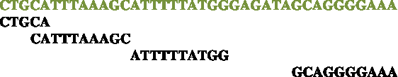
The following diagram illustrates how a DNB arm reads genomic bases in the common case where the wobble gaps are −2, 0, and 6 bases, respectively, beginning from the end of the fragment. Genomic bases are in green and DNB bases are in black. The end of the fragment is on the left and the mate pair gap is on the right.

We indicate with g_l and g_r vectors of the three gap lengths for the left and the right arm, respectively, with g_m the length of the mate gap, and with g the triplet (g_l,g_m,g_r). For each experiment, statistical distributions P(g_l), P(g_r), and P(g_m) are obtained during mapping. We treat those distributions as uncorrelated, and therefore their joint probability distribution is assumed to be \documentclass{aastex}\usepackage{amsbsy}\usepackage{amsfonts}\usepackage{amssymb}\usepackage{bm}\usepackage{mathrsfs}\usepackage{pifont}\usepackage{stmaryrd}\usepackage{textcomp}\usepackage{portland, xspace}\usepackage{amsmath, amsxtra}\pagestyle{empty}\DeclareMathSizes{10}{9}{7}{6}\begin{document} \begin{align*} P (g) = P (g_l) P (g_m) P (g_r) \tag{1} \end{align*} \end{document}

However, the terms P(g_l) and P(g_r) need not decouple into products of probabilities for the individual gap values.

In practice, it is advantageous to allow for gap distributions to also be a function of nearby sequence. However, for simplicity in the presentation of the theory, we will assume that this is not done.

Each base read comes with a quality score which indicates the estimated quality of that base read and which can be converted into an estimated error rate ɛ using a calibration curve obtained during mapping, similar in spirit to the “base quality recalibration” described by DePristo et al. (2011). As the simplest possible assumption, we take this to mean that the genomic base equals the base read in the DNB with probability 1 − ɛ, and any of the three remaining possibilities with probability ɛ /3. More formally, the probability of getting a read b_D for a genomic base b_G is given by \documentclass{aastex}\usepackage{amsbsy}\usepackage{amsfonts}\usepackage{amssymb}\usepackage{bm}\usepackage{mathrsfs}\usepackage{pifont}\usepackage{stmaryrd}\usepackage{textcomp}\usepackage{portland, xspace}\usepackage{amsmath, amsxtra}\pagestyle{empty}\DeclareMathSizes{10}{9}{7}{6}\begin{document} \begin{align*} P (b_D \mid b_G) = \delta (b_{D}, b_G) (1 - \varepsilon) + [ 1 - \delta (b_{D}, b_G) ] \varepsilon / 3 \tag{2} \end{align*} \end{document}

In this expression, δ is the Kronecker symbol defined to be 1 if its two arguments are identical and 0 otherwise.

Our error model also makes the assumption that errors in individual bases within a read are uncorrelated with each other, an assumption justified by our independent sequencing chemistry (Drmanac et al., 2010).

This is the simplest error model possible. As will be apparent, the theory described below does not depend critically on the particular error model chosen. More complex and realistic error models (Wang et al., 2008) could be incorporated without difficulty. The presentation below uses the simplest model both for expositional clarity and because we have not found oversimplification of this component of the model to be among the dominant sources of error for the data we have worked with.

In resequencing assembly, it is assumed that the genome G being sequenced is very similar to a known reference genome G₀. The reference genome is modeled as consisting of a single contiguous sequence of bases with G₀[i] the genome base at position i. Each section of G₀ has an associated ploidy p (p = 1 or 2) which is the number of alleles of that section present in the genome. Here, we do not attempt to estimate ploidy and instead consider it as given at each genome location. We indicate with \documentclass{aastex}\usepackage{amsbsy}\usepackage{amsfonts}\usepackage{amssymb}\usepackage{bm}\usepackage{mathrsfs}\usepackage{pifont}\usepackage{stmaryrd}\usepackage{textcomp}\usepackage{portland, xspace}\usepackage{amsmath, amsxtra}\pagestyle{empty}\DeclareMathSizes{10}{9}{7}{6}\begin{document} $$N_{G_0}$$ \end{document} the total number of bases in the reference genome, summed over all alleles. For the human genome this number is approximately 6 × 10⁹.

The DNB generation process is modeled assuming that each DNB randomly originates at a position of one of the two strands of the genome G being sequenced, and from one of the p alleles at that position, with all strands, positions, and alleles equally likely to originate a DNB. This is a simplifying assumption which could easily be relaxed if a model of bias in DNB generation were available. However this simplification is generally without consequence unless there is strong allele-specific bias at a given site.

A single sequencing experiment generates N_D DNBs for a total of n_DN_D base reads. The average coverage per allele is c = n_DN_D /N_G. In a typical sequencing experiment, c ≈ 20. In this report, we chose to use coverage per allele, instead of the more customary coverage per reference base position, because it results in simpler mathematical equations.

Once the position x, strand s, allele a, and gap values g for a DNB are fixed, each base position in the DNB is mapped to a base position in the genome by a mapping function that, given a DNB base position i, returns the corresponding position in the genome. We assume that the events that generate the gap values g are uncorrelated with those that generate the position x and strand s, and therefore the probability of each mapping is given by \documentclass{aastex}\usepackage{amsbsy}\usepackage{amsfonts}\usepackage{amssymb}\usepackage{bm}\usepackage{mathrsfs}\usepackage{pifont}\usepackage{stmaryrd}\usepackage{textcomp}\usepackage{portland, xspace}\usepackage{amsmath, amsxtra}\pagestyle{empty}\DeclareMathSizes{10}{9}{7}{6}\begin{document} \begin{align*} P [ M (x, s, g, a) ] = \frac {1} {2N_G} P (g). \tag{3} \end{align*} \end{document}

Here, the factor of 2 takes into account the existence of two strands. The existence of two alleles is already taken into account by our definition of N_G.

Due to the possibility of errors, the base read at that DNB position will not always equal the corresponding base in the genome. Based on the error model described above, and under the assumption that the mapping has been fixed, the probability of generating a DNB with base reads b_i is given by a product over the individual base reads \documentclass{aastex}\usepackage{amsbsy}\usepackage{amsfonts}\usepackage{amssymb}\usepackage{bm}\usepackage{mathrsfs}\usepackage{pifont}\usepackage{stmaryrd}\usepackage{textcomp}\usepackage{portland, xspace}\usepackage{amsmath, amsxtra}\pagestyle{empty}\DeclareMathSizes{10}{9}{7}{6}\begin{document} \begin{align*} P (DNB \mid G, M) = \prod_{i}P \{b_i \mid G [ M (i) ] \} \tag{4} \end{align*} \end{document}

Using the error model described by Equation (2) \documentclass{aastex}\usepackage{amsbsy}\usepackage{amsfonts}\usepackage{amssymb}\usepackage{bm}\usepackage{mathrsfs}\usepackage{pifont}\usepackage{stmaryrd}\usepackage{textcomp}\usepackage{portland, xspace}\usepackage{amsmath, amsxtra}\pagestyle{empty}\DeclareMathSizes{10}{9}{7}{6}\begin{document} \begin{align*} P (DNB \mid G, M) = \prod_{i} \Big\{(1 - \varepsilon_{i}) \delta \big[ b_{i}, G (M (i)) \big] + \big[ 1 - \delta [b_{i}, G (M (i))] \big] \varepsilon_{i} / 3 \Big\} \tag{5} \end{align*} \end{document}

In words, each term of the product equals (1 − ɛ_i) if the DNB base equals the genome base at that position, and ɛ_i / 3 otherwise. Here, ɛ_i represents the estimated error rate for the base read at position i.

Combining the previous results, and under the further assumption that the base read process is uncorrelated with the DNB generation process, the probability that a genome G will generate a DNB with base reads b_i is given by \documentclass{aastex}\usepackage{amsbsy}\usepackage{amsfonts}\usepackage{amssymb}\usepackage{bm}\usepackage{mathrsfs}\usepackage{pifont}\usepackage{stmaryrd}\usepackage{textcomp}\usepackage{portland, xspace}\usepackage{amsmath, amsxtra}\pagestyle{empty}\DeclareMathSizes{10}{9}{7}{6}\begin{document} \begin{align*} P (DNB \mid G) = \sum_{M} P (M) P (DNB \mid G, M) = \frac {1} {2N_{G}} \sum_{M} P (g) P (DNB \mid G, M). \tag{6} \end{align*} \end{document}

Here, the sum is extended over all possible mappings of a DNB to G, that is to all possible values of x, s, a, and g. In practice, as we describe below, we make an approximation that allows us to greatly reduce the number of terms in the sum.

Application of Bayes' theorem

Suppose we are given the reference genome G₀ and an hypothetical genome G, assumed to be equally likely a priori. As a result of Bayes' theorem the observation of a single DNB gives a new estimate for the probability ratio: \documentclass{aastex}\usepackage{amsbsy}\usepackage{amsfonts}\usepackage{amssymb}\usepackage{bm}\usepackage{mathrsfs}\usepackage{pifont}\usepackage{stmaryrd}\usepackage{textcomp}\usepackage{portland, xspace}\usepackage{amsmath, amsxtra}\pagestyle{empty}\DeclareMathSizes{10}{9}{7}{6}\begin{document} \begin{align*} \frac {P (G \mid DNB)} {P (G_0 \mid DNB)} = \frac {P (DNB \mid G)} {P (DNB \mid G_0)}. \tag{7} \end{align*} \end{document}

If we assume that all DNBs are generated independently of each other, we can iterate the above and obtain probability estimates that take into account all of the observed DNBs: \documentclass{aastex}\usepackage{amsbsy}\usepackage{amsfonts}\usepackage{amssymb}\usepackage{bm}\usepackage{mathrsfs}\usepackage{pifont}\usepackage{stmaryrd}\usepackage{textcomp}\usepackage{portland, xspace}\usepackage{amsmath, amsxtra}\pagestyle{empty}\DeclareMathSizes{10}{9}{7}{6}\begin{document} \begin{align*} \frac {P (G \mid DNBs)} {P (G_0 \mid DNBs)} = \left(\frac {N_{G_0}} {N_G} \right)^{N_D} \prod_{DNBs} \frac {\sum_MP (g) P (DNB \mid G, M)} {\sum_MP (g) P (DNB \mid G_0, M)} \tag{8} \end{align*} \end{document}

Clearly, it would be straightforward to take into account a priori information, if desired.

Equation (8) allows us to compute the relative probability of any two hypotheses on the genome being sequenced, conditional on the observed DNBs. It is the equation that drives the optimization process described later, which attempts to find genome sequence which maximizes this quantity.

Each term of the product can be evaluated using our DNB generation model (Equation (5)), and this allows us to compute a probability ratio for any two given genomes. However this is expensive because of the large numbers of terms in Equations (6) and (8).

We are assuming that G and G₀ are very similar, and therefore the ratio \documentclass{aastex}\usepackage{amsbsy}\usepackage{amsfonts}\usepackage{amssymb}\usepackage{bm}\usepackage{mathrsfs}\usepackage{pifont}\usepackage{stmaryrd}\usepackage{textcomp}\usepackage{portland, xspace}\usepackage{amsmath, amsxtra}\pagestyle{empty}\DeclareMathSizes{10}{9}{7}{6}\begin{document} $$N_{G_0} / N_G$$ \end{document} is almost exactly equal to 1. If we write \documentclass{aastex}\usepackage{amsbsy}\usepackage{amsfonts}\usepackage{amssymb}\usepackage{bm}\usepackage{mathrsfs}\usepackage{pifont}\usepackage{stmaryrd}\usepackage{textcomp}\usepackage{portland, xspace}\usepackage{amsmath, amsxtra}\pagestyle{empty}\DeclareMathSizes{10}{9}{7}{6}\begin{document} $$N_G = N_{G_0} + \Delta N_G, \ \Delta N_{G_0} / N_G$$ \end{document} is small, and therefore the prefactor in Equation (8) can be written to excellent approximation as \documentclass{aastex}\usepackage{amsbsy}\usepackage{amsfonts}\usepackage{amssymb}\usepackage{bm}\usepackage{mathrsfs}\usepackage{pifont}\usepackage{stmaryrd}\usepackage{textcomp}\usepackage{portland, xspace}\usepackage{amsmath, amsxtra}\pagestyle{empty}\DeclareMathSizes{10}{9}{7}{6}\begin{document} \begin{align*} \left( \frac {N_{G_0}} {N_G} \right)^{N_D} = {exp} \left( - \frac {N_D} {N_{G_0}} \Delta N_G \right) = {exp} \left( - \frac {c} {n_D} \Delta N_G \right) \tag{9} \end{align*} \end{document}

In this expression, c is the average coverage per allele defined above. This means that each extra base in an allele of G causes a decrease in P(G|DNBs) by a factor exp(-c/n_D), even if the remaining factor (the product over all DNBs) does not change. This “insertion penalty” expresses the fact that it does not make sense to add extra bases to G, unless they have sufficient DNB support. Note that the insertion penalty is a direct consequence of the Bayesian model and was not added as an arbitrary additional term.

For compactness we define DNB “weights” \documentclass{aastex}\usepackage{amsbsy}\usepackage{amsfonts}\usepackage{amssymb}\usepackage{bm}\usepackage{mathrsfs}\usepackage{pifont}\usepackage{stmaryrd}\usepackage{textcomp}\usepackage{portland, xspace}\usepackage{amsmath, amsxtra}\pagestyle{empty}\DeclareMathSizes{10}{9}{7}{6}\begin{document} \begin{align*} & W (DNB, G) = \sum_MP (g) P (DNB \mid G, M) \\ & W_0 (DNB) = \sum_MP (g) P (DNB \mid G_0, M). \end{align*} \end{document}

We also define the logarithmic likelihood ratio of G relative to G₀ \documentclass{aastex}\usepackage{amsbsy}\usepackage{amsfonts}\usepackage{amssymb}\usepackage{bm}\usepackage{mathrsfs}\usepackage{pifont}\usepackage{stmaryrd}\usepackage{textcomp}\usepackage{portland, xspace}\usepackage{amsmath, amsxtra}\pagestyle{empty}\DeclareMathSizes{10}{9}{7}{6}\begin{document} \begin{align*} L (G) = log \frac {P (G \mid DNBs)} {P (G_0 \mid DNBs)}. \end{align*} \end{document}

We can then write \documentclass{aastex}\usepackage{amsbsy}\usepackage{amsfonts}\usepackage{amssymb}\usepackage{bm}\usepackage{mathrsfs}\usepackage{pifont}\usepackage{stmaryrd}\usepackage{textcomp}\usepackage{portland, xspace}\usepackage{amsmath, amsxtra}\pagestyle{empty}\DeclareMathSizes{10}{9}{7}{6}\begin{document} \begin{align*} L (G) = - \frac {c} {n_D} \Delta N_G + \sum_{\rm DNBs} log \frac {W (DNB, G)} {W_0 (DNB)} \tag{10} \end{align*} \end{document}

We will measure L(G) and all logarithms of probability ratios in decibels (dB), analogous to the PHRED quality scores used for base calls in sequence traces (Ewing et al., 1998).

Using equation (10), we can in principle compute L(G) for any hypothetical genome G. However, this requires computing, for each DNB, W(G, DNB), and W₀(DNB), which involve sums over all of its possible mappings to G and G₀, regardless of the number of mismatches between the DNB and the hypothetical genomic bases to which it aligns. Therefore, evaluating L(G) has a prohibitive cost O(N_DN_G) which, for fixed coverage, is also equivalent to \documentclass{aastex}\usepackage{amsbsy}\usepackage{amsfonts}\usepackage{amssymb}\usepackage{bm}\usepackage{mathrsfs}\usepackage{pifont}\usepackage{stmaryrd}\usepackage{textcomp}\usepackage{portland, xspace}\usepackage{amsmath, amsxtra}\pagestyle{empty}\DeclareMathSizes{10}{9}{7}{6}\begin{document} $$O (N_G^2)$$ \end{document} . On the other hand, for each DNB only a very small number of mappings are likely to contribute significantly to W(G,DNB) and W(G₀,DNB). This is due to the small multiplying factor ɛ /3 in Equation (5) from each mismatch between the DNB and the genomic base. As a result, only mappings with small numbers of mismatches give a significant contribution. If we have a way of identifying those “good” mappings, we can then extend the sum over those mappings only, and approximate the neglected portion of the sum with a constant α, which is assumed to be the same for all DNBs and independent of G. With this approximation we can write: \documentclass{aastex}\usepackage{amsbsy}\usepackage{amsfonts}\usepackage{amssymb}\usepackage{bm}\usepackage{mathrsfs}\usepackage{pifont}\usepackage{stmaryrd}\usepackage{textcomp}\usepackage{portland, xspace}\usepackage{amsmath, amsxtra}\pagestyle{empty}\DeclareMathSizes{10}{9}{7}{6}\begin{document} \begin{align*} W (G, DNB) = \alpha + \sum_{{\rm good} \ M} P (g) P (DNB \mid G, M) \tag{11} \end{align*} \end{document}

This is a drastic approximation, but its negative effects can be limited with a judicious choice of α and by making a sufficiently inclusive selection of what the “good” mappings are. If the number of “good” mappings per DNB is O(1), the α approximation reduces the computational cost to compute L(G) from quadratic to linear O(N_G) or, equivalently for fixed coverage, O(N_D).

The quantity α has the effect of limiting the amount of contribution a single DNB can give to L(G). For a DNB that does not have any “good” mappings to G₀, W(G₀, DNB) = α. Therefore, if α is chosen to be very small, the ratio W(DNB, G)/W₀ (DNB) can become large, and the contribution of that DNB to L(G) can also become large. As α is increased, the maximum contribution a single DNB can give gets smaller.

In addition to making up for missing mappings, α also captures shortcomings of the probabilistic model. Large values of α result in better robustness in the computation at a price in lost sensitivity to detect true variants.

We note that this Bayesian formulation is different from similar existing approaches based on Bayesian analyses of pile-ups of reads that map at a given locus. Our approach considers all mappings of each DNB to all possible regions of the genome at the same time, and considers alternative alignments of a given mapping. This is particularly important because DNBs, with their variable gaps, often have several mappings of similar quality to a single or multiple regions of the genome.

This formulation is general enough to handle arbitrary choices for G and G₀. In the next section, we show how it is used in practice to compute the relative probability of two genomes differing by one or more neighboring localized SNP or indel variations. However, the results of this formulation are particularly simple in the case where diploid genomes G and G₀ differ by a single, isolated SNP in unique sequence and all base reads have the same error rate ɛ. In this case, with a few more simplifying assumptions, we can express the logarithmic likelihood of a homozygous or heterozygous SNP as simple linear functions of the number of DNB concordant and discordant with the reference: \documentclass{aastex}\usepackage{amsbsy}\usepackage{amsfonts}\usepackage{amssymb}\usepackage{bm}\usepackage{mathrsfs}\usepackage{pifont}\usepackage{stmaryrd}\usepackage{textcomp}\usepackage{portland, xspace}\usepackage{amsmath, amsxtra}\pagestyle{empty}\DeclareMathSizes{10}{9}{7}{6}\begin{document} \begin{align*} & L ({\rm Hom \ SNP}) \approx (n_{disc} - n_{conc}) log \frac {3} {\varepsilon} \\ & L ({\rm Het \ SNP}) \approx n_{conc} log \frac {1} {2} + n_{disc} log \frac {3} {2 \varepsilon} \end{align*} \end{document}

These expressions are reported here for illustration only. They are not otherwise used in this simplified form.

3. Computational Procedures

3.1. Sequence optimization

At least in principle, the Bayesian analysis outlined above allows us to treat DNB assembly as an optimization problem in which we seek to find the genome G that gives the largest possible L(G). In the simplest possible way such a procedure could use greedy optimization and could start with the reference, G = G₀, and then maximize L(G) by iteratively applying one-base changes until convergence to an optimum is reached. However, without refinements such a procedure would be prohibitively expensive in practice.

The computation can be made tractable by separately optimizing one small region at a time, termed the active region. When processing the active region we assume that G = G₀ everywhere outside the active region. With this constraint, we optimize the sequence of G in the active region. The active region is typically chosen to be a few tens of bases long. During optimization, the sequence of each allele in the active region is allowed to diverge arbitrarily from the reference, which allows us to handle simple isolated variations as well as any combination of multiple SNPs and indels in the active region, and overlapping distinct variations on opposite haplotypes.

Under these assumptions, for most DNBs the mappings to G are identical to the mappings to G₀, and therefore W(DNB, G) = W₀(DNB). As a result, most DNBs give no contribution to L(G), as expected. A DNB can contribute to L(G) only if it has “good” mappings to G or G₀ in the active region.

The computation can then be organized by first computing the set of “good” mappings to the reference once, and storing W₀(DNB) for every DNB. To compute W(DNB, G) we first locate potential contributing DNBs by finding DNB arms that map to the reference (and therefore to G) approximately one mate pair away from the active region (Fig. 1). The mate arm of each of these arms is likely to originate from the active region, and therefore it becomes part of a pool of “active arms” that are used for the sequence optimization procedure described below as well as for Local De Novo assembly as described in the next section. For each of these DNBs, we obtain W(DNB, G) by subtracting from W₀(DNB) the contribution of all mappings to G₀ that cover the region of interest, and then adding the contribution of all mappings to G which also cover the active region. In this way, we can compute L(G) using only computations localized to the active region.

FIG. 1.

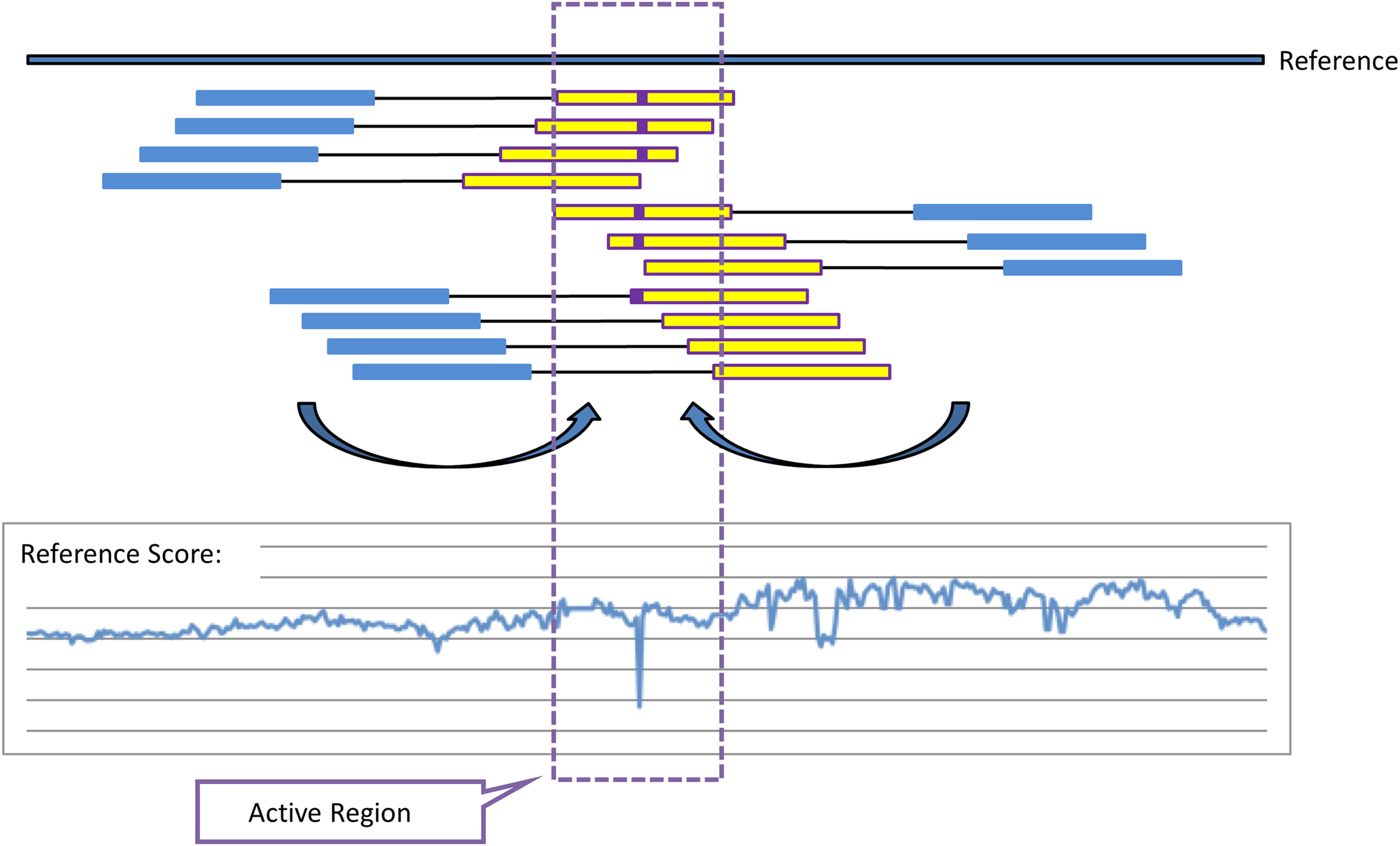
Illustration of mate-based arm-recruitment for reference scoring and definition of active regions, local de novo (LDN) assembly, and optimization. For analysis of a given region of the genome (approximately the yellow interval), mate pairs are identified that have one arm (blue) mapping approximately the expected fragment/mate pair length away from the (yellow) interval of interest, and orientation such that, absent a rearrangement or larger variation, the mated read would be expected to belong in the vicinity of the region of interest. These projected arms are then used to score the hypothesis of homozygous-reference (no variation) against a preliminary set of alternatives, such as all single-base substitutions and indels. In the illustration, mismatches to the reference (purple) lead the homozygous reference hypothesis to be substantially worse than a hypothesized substitution, causing a drop in the reference score, −L(G). The location of this downward spike, padded by a few bases on either side, becomes an active region that is analyzed further.

This makes it feasible to compute L(G) for a relatively large number of hypotheses for the alleles of G in the active region. For each hypothesis, L(G) measures the likelihood of that hypothesis being correct, under the important assumption that G is identical to the reference everywhere outside the active region.

The computation requires a means to quickly find active DNBs that have a good mapping to G in the active region. For this purpose, a local DNB index is used to index all active DNB arms in a way that makes it easy to locate their good mappings to G in the active region. The local DNB index is an associative container that allows fast retrieval of DNB arms based on contained sequence. Selected contiguous segments of arm sequence are used as keys. Its implementation does not present computational problems because of the small number of DNBs involved.

During the optimization process, we can construct local DNB index keys using appropriate sets of bases from G in or near the active region. The hits obtained in the search are combined with mappings of the corresponding non-active arms to G₀ to obtain good mappings of a DNB to G.

This scheme allows the efficient computation of L(G) for any genome G that differs from the reference genome G₀ only in the active region—keeping in mind the assumption mentioned above that the active region must be sufficiently small. With this capability, it is easy to set up a greedy optimization procedure. At each step, we apply to the current p alleles of G all possible one base changes that affect only the active region. This includes changing an individual base position to a different value, deleting it, or inserting a new base to its right or left. If more than one allele is present, this is done in turn for each of the alleles (leaving the remaining allele(s) unchanged). For each modified G obtained in this way we compute L(G) using the procedure described above. We then apply to G the one-base change that resulted in the largest L(G), and iterate until no further improvement in L(G) can be obtained. We store the details of all hypotheses for G that have a computed probability within a given factor of the most likely hypothesis found, up to a maximum number of hypotheses.

The optimization procedures for each active region are all independent and can therefore be executed in parallel, providing a massive degree of parallelism to the assembly procedure.

3.2. Local de novo assembly

The greedy optimization procedure started with alleles equal to the reference often produces the correct answer. However, in some cases it converges to a local optimum of L(G). For this reason, we supplement the optimization procedure with a Local De Novo (LDN) assembly procedure.

The LDN procedure is a De Bruijn graph-based method that uses, for each active region separately, the same pool of active arms used for sequence optimization and recruited as described above and in Figure 1. Note that this is not a double ended assembly: one arm is only used to recruit the DNB, and the other arm is used for assembly.

Existing de novo assembly methods based on De Bruijn graphs (Pevzner et al., 2001) apply only to contiguous reads. A straightforward application of these methods to our read structure would have the effect of neglecting the five bases in the 5-base read of each DNB arm and, more importantly, would not use information about the relative positions of the 10-base reads.

In order to take full advantage of the discontinuous and variably gapped reads of a DNB arm, the De Bruijn graph procedure can be extended as follows. We choose a length n_C (typically around 30 bases) and define a De Bruijn graph with sequences of n_C bases associated to vertices and sequences of n_C + 1 bases associated to edges.

The graph is initialized with vertices, but not edges, using the reference sequence G₀ in the active region. We then expand the graph by recursively adding new edges and vertices adjacent to the edges and vertices already in the graph. For a new edge or vertex to be added the graph we require a minimum number of DNB arms that map, at least partially and without too many mismatches, to the sequences associated with the candidate new edges and vertices. As an example, we might require at least one DNB that has at least 14 bases mapping to the candidate new sequence with at most one mismatch. The same local DNB index described above is used during this process.

In most cases, this recursive procedure is well behaved. However, in some cases, the number of vertices and edges generated can grow exponentially. To prevent that, candidate new vertices are added to a priority queue based on the number of DNB arms that support each vertex and the quality of DNB arm mappings to the vertex sequence. At each step of the recursive procedure, the highest priority vertex is analyzed to determine whether we can construct new edges to or from that vertex. The procedure is stopped either when the queue is empty, meaning that no additional edges or vertices can be added to the graph, or when a specified maximum number of vertices has been created.

When finished, we enumerate paths in the graph that begin and end at the two locations directly adjacent to the active region. Each path provides a new seed for the optimization procedure. The seed can contain an arbitrary combination of SNPs and indels relative to the reference sequence. If we have found a total of n_P paths, including the path corresponding to the reference sequence in that region, there are a total \documentclass{aastex}\usepackage{amsbsy}\usepackage{amsfonts}\usepackage{amssymb}\usepackage{bm}\usepackage{mathrsfs}\usepackage{pifont}\usepackage{stmaryrd}\usepackage{textcomp}\usepackage{portland, xspace}\usepackage{amsmath, amsxtra}\pagestyle{empty}\DeclareMathSizes{10}{9}{7}{6}\begin{document} $${n_P \choose p}$$ \end{document} combinations of p of the seeds, where again p is the ploidy (number of alleles) in the active region. We compute L(G) for each of these combinations. The ones that give the largest values are then used as seeds for the optimization procedure. This limits the number of optimizations that have to be performed, which can be important in cases when the De Bruijn graph is complex and n_P is large.

The results of this graph-based procedure are only used as seeds for the optimization procedure, during which the sequence of both alleles can still be modified arbitrarily.

The LDN procedure increases greatly the success rate of the optimization procedure, particularly if long variations from the reference are present in the active region

3.3. Selecting the active regions

Before sequence optimization runs one active region at a time, we run a preliminary step which determines the set of active regions. This preliminary step computes L(G) for all possible one base-variations in homozygous or heterozygous form. This can include SNPs, as well as one-base insertions and deletions. In addition, we also consider insertions and deletions where one repeat unit in a tandem repeat of period up to 10 bases is inserted or deleted. At most locations, L(G) is computed to be negative, expressing the fact that G₀ is more likely than any one-base variation at that position. However, at positions where a one-base variation is present, L(G) will be computed to be large and positive. The strength of each peak also offers a measure of the strength of the DNB evidence in favor of the corresponding SNP or indel. A similar way of detecting SNPs has been used in the PolyBayes package (Marth et al., 1999). The “reference score”, defined as -max[L(G)] over all hypotheses considered at this stage, can be defined for every base and provides a confidence score for a call of homozygous reference outside of active regions.

This computation would be sufficient if we only wanted to assemble one-base variations, but the situation is complicated by the possibility of longer variations. In regions where a longer variation is present, L(G) for one-base variations is typically still negative, but much less negative than in regions where no variation is present. Such an event in L(G) is used to recognize the possibility of the presence of a variation nearby. All such regions are then added to the list of regions to be optimized.

This algorithm is also complemented by preliminary runs of the graph-based LDN algorithm. The presence of a branch in the graph is also taken to indicate the possibility of a variation being present.

Regions suggested by high L(G) and by the presence of branches in the De Bruijn graph are combined if they are sufficiently close to each other (typically less than the length of a DNB arm), and each of the combined intervals is added to the list of regions to be optimized. However, some of these intervals are too long (e.g., more than 200 bases), and optimizing them would become too expensive. Such intervals are therefore “no-called” without attempting optimization.

3.4. Variation calling

The output of the optimization procedure is, for each of the selected active regions, a list of the most likely hypotheses for the p alleles of G in the active region, together with the corresponding computed L(G). In many cases, each active region ends up with a single hypothesis that is computed to be much more likely than all other hypotheses, and which can then confidently be deemed to describe the correct sequence in the active region. However, it sometimes happens that there are many similar hypotheses, all within a small probability factor of the most likely hypothesis. In such cases, making a call on the sequence of G in the active region is harder.

Individual differences between G and G₀ receive a score (in dB) as follows. The dB separation (logarithm of probability ratio) between the top hypothesis and the first hypothesis not containing a given candidate variation is used as the confidence score for the variation. If the score for a given variation exceeds a threshold, it is output as a called variation along with its score. If the score is below the threshold, a “no-call” (a statement of uncertainty, possibly regarding one allele) is output for the corresponding portion of the reference. The variation score threshold can be chosen to achieve the desired balance of accuracy and sensitivity. In practice, different thresholds, usually 20 and 40 dB, are used for homozygous and heterozygous variations, respectively.

Note that variation calls generated at this phase could still be turned into “no-calls” later during correlation analysis (see the next section).

For simplicity, consider a haploid example where the most likely hypotheses stored are as follows, where the allele corresponding to the reference sequence G₀ is the last one:

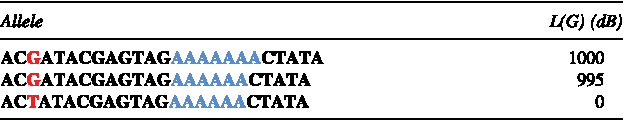
The two most likely hypotheses have a SNP at the position highlighted in red. In addition, the first hypothesis has an insertion of an extra A in the homopolymer run, highlighted in blue. The SNP, present in the two top hypotheses but not in the third, receives a score of 1000 dB. The insertion is present in only the top hypothesis, receiving a score of 5 dB. Therefore, the outcome in this case would be to call the SNP with a score of 1000 dB, but to “no-call” the region with the homopolymer run.

3.5. Correlation analysis

In the majority of cases, working with a single active region at a time is sufficient, as DNBs that have a “good” mapping overlapping a given region will have no other “good” mappings. However, in some cases, two active regions at a time need to be considered due to DNBs having “good” mappings to both regions. Label the two regions 1 and 2, and consider the following genomes:

• G₁ differs from the reference in region 1 but is identical to the reference in region 2.

• G₂ differs from the reference in region 2 but is identical to the reference in region 1.

• G₁₂ differs from the reference in both regions. It is identical to G₁ in region 1 and identical to G₂ in region 2.

In most cases, the equality L(G₁₂) = L(G₁) + L(G₂) will hold (the two active regions are uncorrelated). This equality is exact if the set of DNBs supporting G₁ is disjoint from the set of DNBs supporting G₂. This is the reason that considering one active region at a time is usually sufficient. However, there are three situations where the two sets of supporting DNBs are not disjoint:

• The two active regions are at a distance less than ≈ 40 bases, so a single DNB arm can have mappings that overlap both of them.

• The two active regions are at a distance approximately equal to a mate gap length, so a single DNB can have mappings that overlap both of them.

• The two active regions are at any distance from each other in the genome, but are similar in sequence, exactly or approximately. Because of this similarity it is possible for a single DNB to have “good” mappings to both regions, particularly considering the uncertainty generated by the existence of wobble gaps.

In situations like these, a correlation term appears and L(G₁₂) no longer equals the sum of L(G₁) and L(G₂). The value of the correlation term can reveal information that contradicts the conclusions one would have reached by considering L(G₁) and L(G₂) in isolation. For example, in situations involving regions with high sequence similarity, one can have large, approximately equal values for L(G₁) and L(G₂), while L(G₁₂) is approximately zero. This indicates that one and only one of the two active regions differs from the reference. However, it is unknown which of the two does differ from the reference.

The computation of L(G₁₂) is done only for pairs of active regions that have non-disjoint sets of supporting DNBs. The computation is more complex than when dealing with a single active region, because it involves computing mappings involving both regions. However, it is still the case that W(DNB, G₁₂) can be computed using W₀(DNB) as a basis, by subtracting and adding contributions of mappings involving the two active regions.

This correlation analysis is used as a “correlation filter” to identify regions where probability computations based on a single active region are likely to be unreliable due to sequence similarity with other regions of the genome. In these regions, the variation calling algorithm is not applied. Instead, these regions are no-called. For comments on the composition of regions no-called for this reason, see the Discussion.

As will be shown later, this correlation analysis has an important role for accuracy, and in particular is capable of substantially reducing false positive calls in repetitive regions.

3.6. Summary of computational procedures and comparison to existing approaches

In summary, the resequencing procedure consists of the following steps:

(1) Map DNBs to the reference genome. This mapping step is quite constrained in that it does not allow for insertions and deletions, and only allows a small number of mismatches.

(2) Select active regions to which the LDN procedure and sequence optimization will be applied (see Section 3.3).

(3) For each of these regions, perform the LDN procedure (see Section 3.2) which gives starting seeds for the sequence optimization process. Then optimize the sequences of the two alleles until convergence is achieved (see Section 3.1). These steps use DNBs selected because of a mapping one mate gap away, regardless of how they map to the active region.

(4) Analyze the most likely hypotheses encountered during the optimization process to call variations (see Section 3.4). This can result in no-calling, if competing hypotheses of comparable probability are found.

(5) Turn some of the calls into no-calls under the guidance of correlation analysis (see Section 3.5).

The process differs from the prevailing map-consensus approach in that variation calling is achieved via a local reassembly process and not via read alignment. Our error model allows for uncertainty in local read alignment, in contrast to previous Bayesian methods that compute genotypes for each column in a fixed set of read alignments. This reduces bias towards calling reference sequence, and provides a solution to the multiple-sequence-alignment problem that challenges the map-consensus paradigm. At least one other recent assembly pipeline (DePristo et al., 2011) includes a specific module, “realignment,” with similar motivation. Our process fits within an integrated Bayesian optimization framework, and provides robustness in the face of variations that would prevent direct mapping/alignment of reads to the reference. This latter point is particularly an issue with the gapped nature of reads generated by the Complete Genomics sequencing process, but has broader theoretical applicability to longer insertions and regions of high divergence from the reference. Lastly, the model intrinsically allows for uncertainty in global mapping, permitting the formulation of the correlation analysis (see Section 3.5).

These differences in approach support the variably gapped nature of our reads, in which the longest contiguous read is 10 bases long. On the other hand, we expect that the methods we developed could also be applicable for DNA sequencing technologies other than ours. Software implementing the methods described here is not currently available.

4. Results

The computational procedures described in the previous section have been applied, without additional filtering or other heuristics, to the totality of the genome sequences assembled by Complete Genomics as part of its commercial activities (over 1000 deep-coverage whole human genomes to date) and continue to be used routinely for all production sequencing at Complete Genomics. The results of assemblies generated with this pipeline have been used in a number of published studies (Drmanac et al., 2010; Moore et al., 2011; Rios et al., 2010; Roach et al., 2010; Lee et al., 2010). Sample results for 69 genomes are publicly available on the company's Web site.

At the time of writing, the computation is performed using a subset of a cluster of about 400 multi-core commodity computers connected via 1 Gbit/s Ethernet. Each of the computers has eight processing cores, and the entire process for a single genome typically takes a total of about 2000 core-hours, including the image processing necessary to obtain the base calls and scores of each DNB. The most expensive phase of the computation—the LDN procedure and Bayesian based sequence optimization—can be performed separately for each active region, which gives the procedure a high degree of parallelism. Each assembly can be run with latency of only one or two days using the cluster in parallel. The cluster can perform human assemblies with a throughput of about 20 per day.

The accuracy of the assemblies generated by this procedure has been investigated in detail elsewhere (Drmanac et al., 2010; Roach et al., 2010). Briefly, comparison to Sanger sequencing of novel variants has yielded false positive rate estimates of 2.3–6.1 SNPs/Mbp, 2.3–3.9 insertions/Mbp, and 1.8–3.0 deletions/Mbp (Drmanac et al., 2010). In the same study, 96% of the SNPs on an Illumina Infinium SNP array were called within the whole-genome assembly, with a false negative rate of 0.19% at called loci (excluding regions that are no-called). An independent set of error analyses within a family quartet (Roach et al., 2010) yielded an error estimate within the assemblies of 8.1–11 per Mbp.

It may be possible to improve upon this accuracy by applying additional a posteriori filtering, as described by others (Li et al., 2008; DePristo et al., 2011). We have not investigated this in this article.

4.1. Comparison of using optimization and LDN assembly individually or in combination

The combination of sequence optimization based on Bayes statistics and the LDN technique is essential for robustness and accuracy. The LDN procedure is often successful in finding the correct sequence. However, it is not by itself sufficiently robust, and does not provide a way to evaluate and score different paths in the graph, or different possibilities for the assembled sequence. Attempts to use the LDN procedure by itself in combination with heuristic filtering criteria proved to be only partially successful. Bayesian computations eliminate these shortcomings by providing a robust way to score hypotheses. In addition, the optimization process provides additional paths to the correct solution even in cases where the LDN assembly procedure is not successful. However, the optimization process is also by itself insufficient because it can occasionally converge to an incorrect local optimum.

To illustrate these points, we performed three assemblies of an identical simulated dataset in which SNPs and indels are introduced at a realistic rate. The first assembly is a baseline run in which both optimization and LDN are used. The second used optimization, but starting the optimization with reference sequence instead of also using sequence obtained from LDN. The third simply took the two strongest alleles (as evaluated using the Bayesian model) found by the LDN procedure as the answer, and skipped the optimization. The runs were done using variation calling thresholds of 20 dB for homozygous and 40 dB for heterozygous variations respectively, the values commonly used for production sequencing. The results are summarized in Table 1, from which it is apparent that the combination of Bayesian optimization and LDN assembly techniques gives superior results compared to each of the two techniques used individually.

Table 1.

Comparison of Using Optimization and Local De Novo Assembly Individually or in Combination

Outcome	LDN + optimization	Optimization, no LDN	LDN, no optimization
Both alleles called correctly	4344433	4233437	4335172
One allele called correctly, one no-called	2889	2888	2640
Both alleles no-called	1490837	1606500	1450657
False positive	841	1474	2148
False negative	8435	52611	10330
One allele called correctly, one incorrectly	8308	81158	11774
Both alleles called incorrectly	2068	2746	3024
Other/unclassified	1173	2231	950
Total loci	5850549	5930434	5806365

Results of three simulations in which Bayesian optimization and Local De Novo assembly (LDN) are used in combination or individually. For each of the simulations, the table lists the number of loci in each of the categories described in the Outcome column. Loci are classified by comparing the results of the assembly with the simulated variations. These counts only include loci in which either or both of the simulated and assembled sequence are different from the reference sequence.

4.2. Importance of correlation analysis

To illustrate the importance of correlation analysis, we used a simulation to compare accuracy before and after applying the correlation filter (Table 2). The results show a dramatic improvement in call quality—that is, the correlation filtering step is effective in identifying variations calls that are dubious and are likely to be artifacts of sequence similarity. The large decrease in false positives is a consequence of the fact that most of the false positives incurred without correlation filtering are actually small differences between distinct copies of similar sequence in separate regions of the genome.

Table 2.

Effect of Correlation Analysis

Outcome	Without correlation analysis	With correlation analysis
Identical	4314909 (88.22%)	4203800 (93.05%)
False negative	19434 (0.40%)	10010 (0.22%)
False positive	377550 (7.72%)	681 (0.02%)
Mismatch	6314 (0.13%)	487 (0.01%)
Other/unclassified	172571 (3.53%)	302636 (6.70%)

This table shows the accuracy improvements achieved because of correlation analysis. The variation calls obtained are compared with the simulated sequence and the number of calls with each possible outcome are tabulated. For each outcome, the results are presented as number of calls followed in parenthesis by the proportion of calls. The counts only include loci in which either or both of the simulated and assembled sequence are different from the reference sequence. The last category includes loci where a well-defined outcome could not be defined, typically due to multiple variations at the same locus.

In Table 3, we show the distribution of regions that are no-called due to correlation analysis. While the previous tables reported statistics for simulations, the data in this table refer to a run with real data. The table shows that repeats are overrepresented in these regions. For example, the table shows that of the regions that are no called as a result of correlation analysis, 91.6% are repetitive. Of the human genome, only 52.6% is repetitive. This again illustrates that correlation effects are important when DNBs have more than one mapping.

Table 3.

Characterization of the Regions that Are No-Called as a Result of Correlation Analysis

	Repeats	Segment duplications	Tandem repeats	Any repetitive	Coding	Any
Genome	49.8%	4.8%	2.3%	52.6%	1.2%	53.2%
No-called by correlation analysis	71.0%	39.0%	9.2%	91.5%	1.2%	91.6%

This table shows the concentration in repetitive regions of candidate variations that are ultimately no-called as a result of correlation analysis, as compared to the genome as a whole. The “any repetitive” category combines the three categories to its left (repeats, segment duplications, and tandem repeats), which overlap with one another.

5. Conclusion

We have presented a combination of computational techniques for resequencing that, contrary to existing approaches, accommodates a read structure in which individual contiguous segments are too short to be unique in the reference genome. These methods achieve accuracy and robustness both for isolated small variations and for complex combinations of neighboring sequence variations of short length. Both the theory and the computational methods presented here are general enough that they could also be applied to other sequencing technologies with different read structures. They provide a rigorous approach to handling multiply-mapping reads as well as short regions sufficiently diverged from the reference to prevent mapping of reads.

The approaches described here do not by themselves reconstruct structural variations or longer indels or substitutions (generally, more than several tens of bases). However, in combination with analysis of anomalous paired-end mapping, our extended pipeline (not described here) uses the approach to evaluate and refine hypothesized larger-scale variations including large deletions, insertions of mobile elements, and the junctions (fusions) resulting from other structural variations.

These techniques have been implemented in a computational pipeline that is efficient and highly parallel and that is used routinely for high volume production resequencing of human genomes.

Footnotes

Disclosure Statement

All authors are current or former employees of Complete Genomics and own stock and/or stock options in the company.

References

Bentley

D.R.

, Balasubramanian

, Swerdlow

H.P.

et al. 2008. Accurate whole human genome sequencing using reversible terminator chemistry. Nature, 456:53–59.

Churchill

G.A.

, Lazareva

1999. Bayesian restoration of a hidden Markov chain with applications to DNA sequencing. J. Comput. Biol., 6:261–277.

Churchill

G.A.

, Waterman

M.S.

1992. The accuracy of DNA sequences: estimating sequence quality. Genomics, 14:89–98.

Denisov

, Walenz

, Halpern

A.L.

et al. 2008. Consensus generation and variant detection by Celera Assembler. Bioinformatics, 24:1035–1040.

DePristo

M.A.

, Banks

, Poplin

et al. 2011. A framework for variation discovery and genotyping using next-generation DNA sequencing data. Nat. Genet., 43:491–498.

Drmanac

, Sparks

A.B.

, Callow

M.J.

et al. 2010. Human genome sequencing using unchained base reads on self-assembling DNA nanoarrays. Science, 327:78–81.

Ewing

, Hillier

, Wendl

M.C.

et al. 1998. Base calling of automated sequence traces using PHRED. I. Accuracy assessment. Genome Res., 8:175–185.

Flicek

, Birney

2009. Sense from sequence reads: methods for alignment and assembly. Nat. Methods, 6:S6–S12.

Kim

J.H.

, Waterman

M.S.

, Li

L.M.

2007. Diploid genome reconstruction of Ciona intestinalis and comparative analysis with Ciona savignyi. Genome Res., 17:1101–1110.

10.

Lee

, Jiang

, Liu

et al. 2010. The mutation spectrum revealed by paired genome sequences from a lung cancer patient. Nature, 465:473–477.

11.

Ley

T.J.

, Mardis

E.R.

, Ding

et al. 2008. DNA sequencing of a cytogenetically normal acute myeloid leukaemia genome. Nature, 456:66–72.

12.

, Ruan

, Durbin

2008. Mapping short DNA sequencing reads and calling variants using mapping quality scores. Genome Res., 18:1851–1858.

13.

, Homer

2010. A survey of sequence alignment algorithms for next-generation sequencing. Brief. Bioinform., 11:473–483.

14.

Lupski

J.R.

, Reid

J.G.

, Gonzaga-Jauregui

et al. 2010. Whole-genome sequencing in a patient with Charcot-Marie-Tooth neuropathy. N. Engl. J. Med., 362:1181–1191.

15.

Marth

G.T.

, Korf

, Yandell

M.D.

et al. 1999. A general approach to single-nucleotide polymorphism discovery. Nat. Genet., 23:452–456.

16.

McKenna

, Hanna

, Banks

et al. 2010. The Genome Analysis Toolkit: a MapReduce framework for analyzing next-generation DNA sequencing data. Genome Res., 20:1297–1303.

17.

McKernan

K.J.

, Peckham

H.E.

, Costa

G.L.

et al. 2009. Sequence and structural variation in a human genome uncovered by short-read, massively parallel ligation sequencing using two-base encoding. Genome Res., 19:1527–1541.

18.

Moore

, Hu

, Singleton

et al. 2011. Global analysis of disease-related DNA sequence variation in 10 healthy individuals: implications for whole genome-based clinical diagnostics. Genet. Med., 13:210–217.

19.

Pevzner

P.A.

, Tang

, Waterman

M.S.

2001. An Eulerian path approach to DNA fragment assembly. Proc. Natl. Acad. Sci. USA, 98:9748–9753.

20.

Rios

, Stein

, Shendure

et al. 2010. Identification by whole-genome resequencing of gene defect responsible for severe hypercholesterolemia. Hum. Mol. Genet., 19:4313–4318.

21.

Roach

J.C.

, Glusman

, Smit

A.F.

et al. 2010. Analysis of genetic inheritance in a family quartet by whole-genome sequencing. Science, 328:636–639.

22.

Wang

, Wang

, Li

et al. 2008. The diploid genome sequence of an Asian individual. Nature, 456:60–65.

23.

The 1000 Genomes Project Consortium. 2010. A map of human genome variation from population-scale sequencing. Nature, 467:1061–1073.

Computational Techniques for Human Genome Resequencing Using Mated Gapped Reads

Abstract

Abstract

1. Introduction

2. Theory

Application of Bayes' theorem

3. Computational Procedures

3.1. Sequence optimization

3.2. Local de novo assembly

3.3. Selecting the active regions

3.4. Variation calling

3.5. Correlation analysis

3.6. Summary of computational procedures and comparison to existing approaches

4. Results

4.1. Comparison of using optimization and LDN assembly individually or in combination

4.2. Importance of correlation analysis

5. Conclusion

Footnotes

Disclosure Statement

References