Studying the Evolution of Promoter Sequences: A Waiting Time Problem

Abstract

Abstract

To gain a better understanding of the evolutionary dynamics of regulatory DNA sequences, we address the following questions: (1) How long does it take until a given transcription factor (TF) binding site emerges at random in a promoter sequence? and (2) How does the composition of a TF binding site affect this waiting time? Using two different probabilistic models (an i.i.d. model and a neighbor dependent model), we can compute the expected waiting time for every k-mer, k ranging from 5 to 10, until it appears in a promoter of a species. Our findings indicate that new TF binding sites can be created on a short evolutionary time scale, i.e. in a time span below the speciation time of human and chimp. Furthermore, one can conclude that the composition of a TF binding site plays a crucial role concerning the waiting time until it appears and that the CpG methylation-deamination substitution process probably accelerates the creation of new TF binding sites. A screening of existing TF binding sites moreover reveals that k-mers predicted to have short waiting times occur more frequently than others. Supplementary Material is available at www.libertonline.com/cmb.

1. Introduction

While the evolution of coding DNA sequences has been intensively studied during the last years and plenty of models have been derived to characterize their evolutionary dynamics (Kreitman and Comeron, 1999), the evolution and structure of regulatory DNA sequences still remain poorly understood. One reason for this is that the organization of promoters is much less understood. Promoters are typically located upstream of the gene they regulate. They contain binding sites for regulatory proteins such as transcription factors (TFs). The binding of a TF to a binding sites enables other factors to bind and finally leads to the recruitment (transcriptional activation) or blocking (transcriptional repression) of the RNA polymerase which is responsible for transcribing the corresponding gene (Wray et al., 2003). TF binding sites are short stretches of DNA. They are distributed sparsely and unevenly and they may overlap partially but sometimes the spacing between two binding sites may be tens of kilobases (kb) as stated by Wray et al. (2003). So the length and composition of a promoter can vary considerably.

Due to these complications, developing a probabilistic model for promoter sequences and describing the evolutionary dynamics of regulatory regions remains a challenge. However, there is growing body of experimental evidence that promoter regions are highly dynamic and that significant changes in gene regulation can occur on a microevolutionary time scale. For example, using ChIP-chip technology, Odom et al. (2007) inferred the binding sites of four tissue-specific TFs in human and mouse liver cells and found that despite the conserved function and motif of these TFs, 41–89% of the binding events are species specific. Taylor et al. (2006) investigated the evolutionary trends of mammalian promoters using large sets of experimentally supported transcription start sites and concluded that the evolution within mammalian promoters has been relatively rapid within approximately the last 25 Myrs.

In order to give a probabilistic explanation for the speed of cis-regulatory evolution, we address the following two questions: (1) How long does it take until a given TF binding site appears at random due to the evolutionary process of single nucleotide mutations? (2) How does the composition of a TF binding site affect this waiting time?

Stone and Wray (2001) tried to answer the first question by simulating the evolution of a promoter region of length 2,000 bp assuming a mutation rate of 10⁻⁹ per nucleotide per generation. After having estimated the waiting time for a 6-mer to emerge in a given promoter sequence, they divide this number by 10⁶ · 2 (=effective population size times two DNA strands) yielding that on average it takes 6,000 years until a 6-mer appears in a promoter sequence of at least one individual in a human population. Their approach of simply dividing by the number of individuals has been critized by MacArthur and Brookfield (2004) and by Durrett and Schmidt (2007), especially because with this, Stone and Wray (2001) implicitly assume that the DNA sequences in a population evolve independently from each other. But indeed, two randomly chosen individuals differ only in 0.1% of their DNA as stated in Durrett and Schmidt (2007). Durrett and Schmidt (2007) tackeld the problem by using a proper population genetics model (the Moran model) and (Poisson) approximated the expected waiting time until a word of fixed length 6 or 8 appears in a promoter region of length 1000 bp in at least one individual in a population of effective size 10⁴. Assuming a mutation rate of 10⁻⁸, Durrett and Schmidt (2007) computed that the expected waiting time for words of length 6 is 100,000 years and 375,000 years for words of length 8 given that there is a 7 out of 8 letter match in the population consensus sequence.

These results are helpful for getting a general idea of how fast TF binding sites can emerge - at least for binding sites of length 6 and 8. However, they rely on the assumption that once a TF binding site is created in one individual, it will confer a substantial benefit and hence, will spread rapidly through the population. But according to population genetics theory (Ewens, 2004) this event only occurs with a small probability: Let us assume for simplicity, that there are only two different individuals A and B in a population of size N where A symbolizes the individual with the new TF binding site appearing only once and B represents the remaining N − 1 individuals without the new TF binding. The fixation probability of A is then given by \documentclass{aastex}\usepackage{amsbsy}\usepackage{amsfonts}\usepackage{amssymb}\usepackage{bm}\usepackage{mathrsfs}\usepackage{pifont}\usepackage{stmaryrd}\usepackage{textcomp}\usepackage{portland,xspace}\usepackage{amsmath,amsxtra}\pagestyle{empty}\DeclareMathSizes{10}{9}{7}{6} \begin{document} \begin{align*} \rho_A = \frac{1 - r^{- 1}}{1 - r^{- N}} \tag {1} \end{align*} \end{document}

where r is the relative fitness of individual A, i.e., the average number of surviving progeny of A compared to B after one generation; see e.g. section 6.3 in Nowak (2006). Setting N = 10⁴ and assuming a relative fitness of 2 (100% selective advantage), the probability that the new TF binding site will get fixed in a population is only 0.5. Even when assuming a very high and unrealistic relative fitness of 10 the fixation probability is just 0.9. Thus, their assumption that a TF binding site once created will spread throughout the population is hard to justify.

In this work, we phrase the question differently. Instead of computing the waiting time until a given TF binding site emerges in a promoter sequence in at least one individual in a population, we are interested in determining the expected waiting time until a given TF binding site gets fixed in a species (assuming that fixation only occurs at the nucleotide/dinucleotide level) - either in one given promoter sequence or in at least one of several promoters, for example, in any or all of the human promoters. As mentioned above, two randomly chosen individuals differ only in 0.1% of their DNA. Therefore, it is reasonable to refer, for example, to the ”human genome.” With this in mind, in our model a DNA sequence should not be interpreted as a sequence of a single individual of a population but as a representative sequence of the considered species. Hence, waiting times relate to appearance in the species instead of appearance in one single individual. Starting with a muliple species alignment for the three species Homo sapiens, Pan troglodytes and Macaca mulatta, we can estimate the evolutionary substitution rates (=fixed mutation rates) for every nucleotide using the Maximum likelihood based tool developed by Arndt and Hwa (2005). As a consequence, for every k-mer, k ranging from 5 to 10, we can (almost) exactly compute its expected waiting time to appear in a species' promoter of a given length in dependence of its composition.

Since the CpG methylation-deamination process (CG → TG and CG → CA) is the predominant evolutionary substitution process, as a second step, we also incorporate neighbor dependent substitution rates into our model. For example, Wang et al. (1998) pointed out that single-nucleotide polymorphisms occur about 10 times more often at CpG dinucleotides than at other dinucleotides in the human DNA. Our approach of calculating waiting times in dependency of the promoter's and TF binding site's composition sheds new light on the process of TF binding site emergence and therefore, extends the previous knowledge about the dynamics of promoter sequence evolution.

As a last step, we compare k-mers which are predicted to appear rapidly according to our model with existing TF binding sites from the database JASPAR (Portales-Casamar et al., 2010). We show that k-mers with short waiting times are used more frequently as TF binding sites than those with long waiting times.

This article is organized as follows: in Section 2.1 we introduce two probabilistic models - an i.i.d. model (model M0) and a model taking the neighbor dependencies of nucleotides into account (model M1). Section 2.2 is devoted to the computation of the expected waiting time under our given models, and in Section 2.3, we explain how one can estimate the model parameters. Utilizing these parameter estimations, in Section 3 we provide the expected waiting times for k-mers, k ranging from 5 to 10, for model M0 and then present the more interesting results for model M1 in detail. Additionally, we relate these k-mers to existing TF binding sites from the database JASPAR (Portales-Casamar et al., 2010). Section 4 discusses the results and explains the impact of our findings.

2. Methods

2.1. The probabilistic model

In order to formalize the problem, one has to model two components: the initial promoter sequence \documentclass{aastex}\usepackage{amsbsy}\usepackage{amsfonts}\usepackage{amssymb}\usepackage{bm}\usepackage{mathrsfs}\usepackage{pifont}\usepackage{stmaryrd}\usepackage{textcomp}\usepackage{portland,xspace}\usepackage{amsmath,amsxtra}\pagestyle{empty}\DeclareMathSizes{10}{9}{7}{6} \begin{document}$$X_1 ( 0 ) , \ldots , X_n ( 0 )$$\end{document} and the time evolution \documentclass{aastex}\usepackage{amsbsy}\usepackage{amsfonts}\usepackage{amssymb}\usepackage{bm}\usepackage{mathrsfs}\usepackage{pifont}\usepackage{stmaryrd}\usepackage{textcomp}\usepackage{portland,xspace}\usepackage{amsmath,amsxtra}\pagestyle{empty}\DeclareMathSizes{10}{9}{7}{6} \begin{document}$$( X_1 ( t ) , \ldots , X_n ( t ) ) _{t \geq 0}$$\end{document} of this sequence.

2.1.1. Modelling the initial promoter sequence

Let \documentclass{aastex}\usepackage{amsbsy}\usepackage{amsfonts}\usepackage{amssymb}\usepackage{bm}\usepackage{mathrsfs}\usepackage{pifont}\usepackage{stmaryrd}\usepackage{textcomp}\usepackage{portland,xspace}\usepackage{amsmath,amsxtra}\pagestyle{empty}\DeclareMathSizes{10}{9}{7}{6} \begin{document}$${ \cal A} = \{ {\rm A , C , G , T}\}$$\end{document} contain the four different bases and let \documentclass{aastex}\usepackage{amsbsy}\usepackage{amsfonts}\usepackage{amssymb}\usepackage{bm}\usepackage{mathrsfs}\usepackage{pifont}\usepackage{stmaryrd}\usepackage{textcomp}\usepackage{portland,xspace}\usepackage{amsmath,amsxtra}\pagestyle{empty}\DeclareMathSizes{10}{9}{7}{6} \begin{document}$$X_1 (0) , \ldots , X_n (0)$$\end{document} be a random promoter sequence of length n which is either modelled by an independent, identically distributed sequence (model M0) or a homogeneous stationary Markov chain of order 1 (model M1).

In model M0, the probability of observing a sequence \documentclass{aastex}\usepackage{amsbsy}\usepackage{amsfonts}\usepackage{amssymb}\usepackage{bm}\usepackage{mathrsfs}\usepackage{pifont}\usepackage{stmaryrd}\usepackage{textcomp}\usepackage{portland,xspace}\usepackage{amsmath,amsxtra}\pagestyle{empty}\DeclareMathSizes{10}{9}{7}{6} \begin{document}$$(x_1 , \ldots , x_n)$$\end{document} is given by \documentclass{aastex}\usepackage{amsbsy}\usepackage{amsfonts}\usepackage{amssymb}\usepackage{bm}\usepackage{mathrsfs}\usepackage{pifont}\usepackage{stmaryrd}\usepackage{textcomp}\usepackage{portland,xspace}\usepackage{amsmath,amsxtra}\pagestyle{empty}\DeclareMathSizes{10}{9}{7}{6} \begin{document} \begin{align*} \mu(x_1, \ldots, x_n ) = \nu (x_1) \cdot \ldots \cdot \nu (x_n). \tag{2} \end{align*}\end{document}

where \documentclass{aastex}\usepackage{amsbsy}\usepackage{amsfonts}\usepackage{amssymb}\usepackage{bm}\usepackage{mathrsfs}\usepackage{pifont}\usepackage{stmaryrd}\usepackage{textcomp}\usepackage{portland,xspace}\usepackage{amsmath,amsxtra}\pagestyle{empty}\DeclareMathSizes{10}{9}{7}{6} \begin{document}$$\nu (x) = P (X_1 (0) = x)$$\end{document} .

In model M1, when \documentclass{aastex}\usepackage{amsbsy}\usepackage{amsfonts}\usepackage{amssymb}\usepackage{bm}\usepackage{mathrsfs}\usepackage{pifont}\usepackage{stmaryrd}\usepackage{textcomp}\usepackage{portland,xspace}\usepackage{amsmath,amsxtra}\pagestyle{empty}\DeclareMathSizes{10}{9}{7}{6} \begin{document}$$X_1 (0) , \ldots , X_n (0)$$\end{document} is a homogeneous stationary Markov chain with stationary distribution ν and transition probabilities \documentclass{aastex}\usepackage{amsbsy}\usepackage{amsfonts}\usepackage{amssymb}\usepackage{bm}\usepackage{mathrsfs}\usepackage{pifont}\usepackage{stmaryrd}\usepackage{textcomp}\usepackage{portland,xspace}\usepackage{amsmath,amsxtra}\pagestyle{empty}\DeclareMathSizes{10}{9}{7}{6} \begin{document}$$\pi_{a , b} , \ a , b \in{\cal A}$$\end{document} , this probability can be computed by \documentclass{aastex}\usepackage{amsbsy}\usepackage{amsfonts}\usepackage{amssymb}\usepackage{bm}\usepackage{mathrsfs}\usepackage{pifont}\usepackage{stmaryrd}\usepackage{textcomp}\usepackage{portland,xspace}\usepackage{amsmath,amsxtra}\pagestyle{empty}\DeclareMathSizes{10}{9}{7}{6} \begin{document} \begin{align*} \mu(x_1, \ldots, x_n ) = \nu(x_1) \pi_{x_1, x_2} \cdot \ldots \cdot \pi_{x_{n - 1}, x_n}. \tag{3} \end{align*}\end{document}

2.1.2. Modelling the time evolution of the promoter sequence

The promoter sequence evolution \documentclass{aastex}\usepackage{amsbsy}\usepackage{amsfonts}\usepackage{amssymb}\usepackage{bm}\usepackage{mathrsfs}\usepackage{pifont}\usepackage{stmaryrd}\usepackage{textcomp}\usepackage{portland,xspace}\usepackage{amsmath,amsxtra}\pagestyle{empty}\DeclareMathSizes{10}{9}{7}{6} \begin{document}$$(X_1 (t) , \ldots , X_n (t)) _{t \geq 0}$$\end{document} is modelled according to the nucleotide substitution model by Arndt et al. (2003) - either taking the CpG methylation-deamination rates into account (model M1) or not (model M0).

In model M0, one only considers the independently evolving nucleotides (12 substitution rates). Since nucleotide substitutions on one strand of the DNA go along with nucleotide substitutions on the complementary strand in order to guarantee correct Watson – Crick base pairing, the number of free parameters is 6 (A → T/T → A, C → G/G → C, A → C/T → G, C → A/G → T, A → G/T → C, G → A/C → T). If Q denotes the 4 × 4 rate matrix, the matrix \documentclass{aastex}\usepackage{amsbsy}\usepackage{amsfonts}\usepackage{amssymb}\usepackage{bm}\usepackage{mathrsfs}\usepackage{pifont}\usepackage{stmaryrd}\usepackage{textcomp}\usepackage{portland,xspace}\usepackage{amsmath,amsxtra}\pagestyle{empty}\DeclareMathSizes{10}{9}{7}{6} \begin{document}$${\mathbb P} (t)$$\end{document} containing the transition probabilities of a evolving into b in finite time t ≥ 0, \documentclass{aastex}\usepackage{amsbsy}\usepackage{amsfonts}\usepackage{amssymb}\usepackage{bm}\usepackage{mathrsfs}\usepackage{pifont}\usepackage{stmaryrd}\usepackage{textcomp}\usepackage{portland,xspace}\usepackage{amsmath,amsxtra}\pagestyle{empty}\DeclareMathSizes{10}{9}{7}{6} \begin{document}$$a , b \in{\cal A}$$\end{document} , is then given by the matrix exponential \documentclass{aastex}\usepackage{amsbsy}\usepackage{amsfonts}\usepackage{amssymb}\usepackage{bm}\usepackage{mathrsfs}\usepackage{pifont}\usepackage{stmaryrd}\usepackage{textcomp}\usepackage{portland,xspace}\usepackage{amsmath,amsxtra}\pagestyle{empty}\DeclareMathSizes{10}{9}{7}{6} \begin{document}$${\mathbb P} (t) = e^{tQ}$$\end{document} ; see e.g. Karlin and Taylor (1975). In this model, the probability of sequence \documentclass{aastex}\usepackage{amsbsy}\usepackage{amsfonts}\usepackage{amssymb}\usepackage{bm}\usepackage{mathrsfs}\usepackage{pifont}\usepackage{stmaryrd}\usepackage{textcomp}\usepackage{portland,xspace}\usepackage{amsmath,amsxtra}\pagestyle{empty}\DeclareMathSizes{10}{9}{7}{6} \begin{document}$$(x_1 , \ldots , x_n)$$\end{document} evolving into \documentclass{aastex}\usepackage{amsbsy}\usepackage{amsfonts}\usepackage{amssymb}\usepackage{bm}\usepackage{mathrsfs}\usepackage{pifont}\usepackage{stmaryrd}\usepackage{textcomp}\usepackage{portland,xspace}\usepackage{amsmath,amsxtra}\pagestyle{empty}\DeclareMathSizes{10}{9}{7}{6} \begin{document}$$(y_1 , \ldots , y_n)$$\end{document} is given by \documentclass{aastex}\usepackage{amsbsy}\usepackage{amsfonts}\usepackage{amssymb}\usepackage{bm}\usepackage{mathrsfs}\usepackage{pifont}\usepackage{stmaryrd}\usepackage{textcomp}\usepackage{portland,xspace}\usepackage{amsmath,amsxtra}\pagestyle{empty}\DeclareMathSizes{10}{9}{7}{6} \begin{document} \begin{align*} p_{(x_1, \ldots, x_{n}) \rightarrow (y_1, \ldots, y_n)} (t) = \prod_{i = 1}^n p_{x_i, y_i} (t).\tag{4} \end{align*} \end{document}

In model M1, we incorporate one particular neighbor dependent substitution process: the CpG methylation-deamination process. That is, apart from the 12 substitution rates mentioned above (given by 6 parameters), one also has 2 other rates (CG → TG and CG → CA) which are assumed to be the same. This results into looking at trinucleotides (nucleotide plus left and right neighbor) whose dynamics are governed by a 64 × 64 rate matrix Q⁽³⁾; for details see Duret and Arndt (2008). For t ≥ 0, the matrix \documentclass{aastex}\usepackage{amsbsy}\usepackage{amsfonts}\usepackage{amssymb}\usepackage{bm}\usepackage{mathrsfs}\usepackage{pifont}\usepackage{stmaryrd}\usepackage{textcomp}\usepackage{portland,xspace}\usepackage{amsmath,amsxtra}\pagestyle{empty}\DeclareMathSizes{10}{9}{7}{6} \begin{document} \begin{align*} {\mathbb P}^{(3)}(t) = (p_{a_1a_2a_3, b_1b_2b_3} (t))_{a_1, \ldots , b_3 \in {\cal A}}\tag{5} \end{align*}\end{document}

is given by \documentclass{aastex}\usepackage{amsbsy}\usepackage{amsfonts}\usepackage{amssymb}\usepackage{bm}\usepackage{mathrsfs}\usepackage{pifont}\usepackage{stmaryrd}\usepackage{textcomp}\usepackage{portland,xspace}\usepackage{amsmath,amsxtra}\pagestyle{empty}\DeclareMathSizes{10}{9}{7}{6} \begin{document}$${\mathbb P}^{(3)} (t) = e^{tQ^{(3)}}$$\end{document} . Applying this, one can compute the probability of a₂ flanked by a₁ and a₃ evolving into b₂ in finite time t ≥ 0 by marginalizing over b₁ and b₃: \documentclass{aastex}\usepackage{amsbsy}\usepackage{amsfonts}\usepackage{amssymb}\usepackage{bm}\usepackage{mathrsfs}\usepackage{pifont}\usepackage{stmaryrd}\usepackage{textcomp}\usepackage{portland,xspace}\usepackage{amsmath,amsxtra}\pagestyle{empty}\DeclareMathSizes{10}{9}{7}{6} \begin{document} \begin{align*} p_{a_1a_2a_3, b_2} (t) = \sum_{b_1, b_3 \in{\cal A}}p_{a_1 a_2 a_3 , b_1 b_2 b_3} (t). \tag{6} \end{align*}\end{document}

In model M1, referring to Arndt and Hwa (2005), Duret and Arndt (2008) the probability of sequence \documentclass{aastex}\usepackage{amsbsy}\usepackage{amsfonts}\usepackage{amssymb}\usepackage{bm}\usepackage{mathrsfs}\usepackage{pifont}\usepackage{stmaryrd}\usepackage{textcomp}\usepackage{portland,xspace}\usepackage{amsmath,amsxtra}\pagestyle{empty}\DeclareMathSizes{10}{9}{7}{6} \begin{document} $$(x_1 , \ldots , x_n)$$\end{document} evolving into \documentclass{aastex}\usepackage{amsbsy}\usepackage{amsfonts}\usepackage{amssymb}\usepackage{bm}\usepackage{mathrsfs}\usepackage{pifont}\usepackage{stmaryrd}\usepackage{textcomp}\usepackage{portland,xspace}\usepackage{amsmath,amsxtra}\pagestyle{empty}\DeclareMathSizes{10}{9}{7}{6} \begin{document}$$(y_1 , \ldots , y_n)$$\end{document} where x₁ is preceded by x₀ and x_n is followed by x_n+1 in finite time t ≥ 0 can then very reliably be approximated by \documentclass{aastex}\usepackage{amsbsy}\usepackage{amsfonts}\usepackage{amssymb}\usepackage{bm}\usepackage{mathrsfs}\usepackage{pifont}\usepackage{stmaryrd}\usepackage{textcomp}\usepackage{portland,xspace}\usepackage{amsmath,amsxtra}\pagestyle{empty}\DeclareMathSizes{10}{9}{7}{6} \begin{document} \begin{align*} p_{(x_0, \ldots , x_{n + 1} ) \rightarrow (y_1 , \ldots , y_n )} (t) \approx \prod_{i = 1}^np_{x_{i - 1}x_ix_{i + 1} , y_i} (t). \tag{7} \end{align*}\end{document}

2.2. The expected waiting time

Let \documentclass{aastex}\usepackage{amsbsy}\usepackage{amsfonts}\usepackage{amssymb}\usepackage{bm}\usepackage{mathrsfs}\usepackage{pifont}\usepackage{stmaryrd}\usepackage{textcomp}\usepackage{portland,xspace}\usepackage{amsmath,amsxtra}\pagestyle{empty}\DeclareMathSizes{10}{9}{7}{6} \begin{document} \begin{align*} b = (b_1, \ldots, b_k) \quad {\rm where} \ b_1 , \ldots , b_k \in {\cal A} \tag{8} \end{align*}\end{document}

be a TF binding site of length k. We want to answer the question: provided that the binding site is not present in the initial sequence \documentclass{aastex}\usepackage{amsbsy}\usepackage{amsfonts}\usepackage{amssymb}\usepackage{bm}\usepackage{mathrsfs}\usepackage{pifont}\usepackage{stmaryrd}\usepackage{textcomp}\usepackage{portland,xspace}\usepackage{amsmath,amsxtra}\pagestyle{empty}\DeclareMathSizes{10}{9}{7}{6} \begin{document}$$X_1 (0) , \ldots , X_n (0)$$\end{document} , how long does one have to wait for \documentclass{aastex}\usepackage{amsbsy}\usepackage{amsfonts}\usepackage{amssymb}\usepackage{bm}\usepackage{mathrsfs}\usepackage{pifont}\usepackage{stmaryrd}\usepackage{textcomp}\usepackage{portland,xspace}\usepackage{amsmath,amsxtra}\pagestyle{empty}\DeclareMathSizes{10}{9}{7}{6} \begin{document}$$b = (b_1 , \ldots , b_k)$$\end{document} to occur randomly during the time evolution of the sequence? We assume a discrete time scale \documentclass{aastex}\usepackage{amsbsy}\usepackage{amsfonts}\usepackage{amssymb}\usepackage{bm}\usepackage{mathrsfs}\usepackage{pifont}\usepackage{stmaryrd}\usepackage{textcomp}\usepackage{portland,xspace}\usepackage{amsmath,amsxtra}\pagestyle{empty}\DeclareMathSizes{10}{9}{7}{6} \begin{document}$${\mathbb N}$$\end{document} corresponding to the number of generations, i.e. we ask how many generations it takes for b to appear for the first time. Thus, one has to determine the distribution of \documentclass{aastex}\usepackage{amsbsy}\usepackage{amsfonts}\usepackage{amssymb}\usepackage{bm}\usepackage{mathrsfs}\usepackage{pifont}\usepackage{stmaryrd}\usepackage{textcomp}\usepackage{portland,xspace}\usepackage{amsmath,amsxtra}\pagestyle{empty}\DeclareMathSizes{10}{9}{7}{6} \begin{document} \begin{align*} T = \inf \{ t \in {\mathbb N}: \exists i \in \{ 1 , \ldots , n - k + 1 \} \ \hbox{such that} ( X_i (t) , \ldots , X_{i + k - 1} (t)) = (b_1 , \ldots , b_k) \} \tag{9} \end{align*}\end{document}

given that b is not present in the initial sequence \documentclass{aastex}\usepackage{amsbsy}\usepackage{amsfonts}\usepackage{amssymb}\usepackage{bm}\usepackage{mathrsfs}\usepackage{pifont}\usepackage{stmaryrd}\usepackage{textcomp}\usepackage{portland,xspace}\usepackage{amsmath,amsxtra}\pagestyle{empty}\DeclareMathSizes{10}{9}{7}{6} \begin{document} $$X_1 (0) , \ldots , X_n (0)$$\end{document} . As shown in Supplementary Material S1 (for all Supplementary Material, see www.libertonline.com/cmb), the distribution of T is approximately a geometric distribution with parameter \documentclass{aastex}\usepackage{amsbsy}\usepackage{amsfonts}\usepackage{amssymb}\usepackage{bm}\usepackage{mathrsfs}\usepackage{pifont}\usepackage{stmaryrd}\usepackage{textcomp}\usepackage{portland,xspace}\usepackage{amsmath,amsxtra}\pagestyle{empty}\DeclareMathSizes{10}{9}{7}{6} \begin{document} \begin{align*} q = {\mathbb P} (b \ \hbox{occurs in generation 1} \mid b \ \hbox{does not occur in generation 0}).\tag{10} \end{align*}\end{document}

Especially, one obtains \documentclass{aastex}\usepackage{amsbsy}\usepackage{amsfonts}\usepackage{amssymb}\usepackage{bm}\usepackage{mathrsfs}\usepackage{pifont}\usepackage{stmaryrd}\usepackage{textcomp}\usepackage{portland,xspace}\usepackage{amsmath,amsxtra}\pagestyle{empty}\DeclareMathSizes{10}{9}{7}{6} \begin{document} \begin{align*} {\mathbb E} (T) \approx \frac {1} {q} .\tag{11} \end{align*}\end{document}

Let \documentclass{aastex}\usepackage{amsbsy}\usepackage{amsfonts}\usepackage{amssymb}\usepackage{bm}\usepackage{mathrsfs}\usepackage{pifont}\usepackage{stmaryrd}\usepackage{textcomp}\usepackage{portland,xspace}\usepackage{amsmath,amsxtra}\pagestyle{empty}\DeclareMathSizes{10}{9}{7}{6} \begin{document} $$B_0^c = \{b \ \hbox{does not occur in generation 0}\}$$\end{document} . To compute q, one has to apply the inclusion-exclusion principle, i.e. \documentclass{aastex}\usepackage{amsbsy}\usepackage{amsfonts}\usepackage{amssymb}\usepackage{bm}\usepackage{mathrsfs}\usepackage{pifont}\usepackage{stmaryrd}\usepackage{textcomp}\usepackage{portland,xspace}\usepackage{amsmath,amsxtra}\pagestyle{empty}\DeclareMathSizes{10}{9}{7}{6} \begin{document} \begin{align*} q &= {\mathbb P} \left( \bigcup_{i = 1}^{n - k + 1} \{( X_i ( 1 ), \ldots , X_{i + k - 1} (1) ) = (b_1 , \ldots , b_k) \} \mid B_0^c \right) \\ &= \sum_{l = 1}^{n - k + 1} (- 1) ^{\ell + 1} \sum_{I \subset \{1 , \ldots , n - k + 1 \} , \mid I \mid = \ell} \underbrace{{\mathbb P} \left( \bigcap_{i \in I} \{ ( X_i (1) , \ldots , X_{i + k - 1} (1)) = ( b_1 , \ldots , b_k ) \} \mid B_0^c \right).}_{ \mathop{ \rm def} \limits_{ =} {p_ \ell}} \tag{12} \end{align*}\end{document}

In both models M0 and M1, the probability p_l indeed only depends on ℓ since we have assumed stationarity. It is the probability of b appearing at ℓ given positions in generation 1 under the condition that it was not present in the generation before. Exact computation of p_ℓ becomes infeasible if the binding site can overlap with itself since computing the probability that b appears ℓ times in generation 1 given that it did not occur in generation 0 requires inspection of many possiblities: b can occur ℓ times with no overlap in generation 1, b can occur ℓ times in one big overlapping clump, b can occur m times in one clump and ℓ − m times in another clump etc. But, of course, for large ℓ the probability p_ℓ becomes very small, so q is dominated by the first summands. Since overlaps can be neglected for small ℓ, for ease of exposition, we neglect the possibility of b occuring self-overlapping. Thus, we use the following approximation \documentclass{aastex}\usepackage{amsbsy}\usepackage{amsfonts}\usepackage{amssymb}\usepackage{bm}\usepackage{mathrsfs}\usepackage{pifont}\usepackage{stmaryrd}\usepackage{textcomp}\usepackage{portland,xspace}\usepackage{amsmath,amsxtra}\pagestyle{empty}\DeclareMathSizes{10}{9}{7}{6} \begin{document} \begin{align*} p_ \ell \approx {\mathbb P} \left(\bigcap_{i \in I} \{ ( X_i (1), \ldots , X_{i + k - 1} (1) ) = (b_1 , \ldots , b_k)\} \mid B_0^c \right) \cdot {\mathbb l}_{\{\mid i - j \mid \geq k \ \hbox{for all}i , j \in I\} }.\tag{13} \end{align*}\end{document}

Due to the assumption that b cannot appear self-overlapping, b can occur at most \documentclass{aastex}\usepackage{amsbsy}\usepackage{amsfonts}\usepackage{amssymb}\usepackage{bm}\usepackage{mathrsfs}\usepackage{pifont}\usepackage{stmaryrd}\usepackage{textcomp}\usepackage{portland,xspace}\usepackage{amsmath,amsxtra}\pagestyle{empty}\DeclareMathSizes{10}{9}{7}{6} \begin{document}$$\lfloor \frac {n} { k } \rfloor$$\end{document} times in the sequence. The number of possible subsets \documentclass{aastex}\usepackage{amsbsy}\usepackage{amsfonts}\usepackage{amssymb}\usepackage{bm}\usepackage{mathrsfs}\usepackage{pifont}\usepackage{stmaryrd}\usepackage{textcomp}\usepackage{portland,xspace}\usepackage{amsmath,amsxtra}\pagestyle{empty}\DeclareMathSizes{10}{9}{7}{6} \begin{document}$$I \subset \{1 , \ldots , n - k + 1\} $$\end{document} with |i − j| ≥ k for all i, \documentclass{aastex}\usepackage{amsbsy}\usepackage{amsfonts}\usepackage{amssymb}\usepackage{bm}\usepackage{mathrsfs}\usepackage{pifont}\usepackage{stmaryrd}\usepackage{textcomp}\usepackage{portland,xspace}\usepackage{amsmath,amsxtra}\pagestyle{empty}\DeclareMathSizes{10}{9}{7}{6} \begin{document}$$j \in I$$\end{document} and |I| = ℓ is \documentclass{aastex}\usepackage{amsbsy}\usepackage{amsfonts}\usepackage{amssymb}\usepackage{bm}\usepackage{mathrsfs}\usepackage{pifont}\usepackage{stmaryrd}\usepackage{textcomp}\usepackage{portland,xspace}\usepackage{amsmath,amsxtra}\pagestyle{empty}\DeclareMathSizes{10}{9}{7}{6} \begin{document}$${n - (k - 1) \cdot \ell \choose \ell}$$\end{document} . Thus, \documentclass{aastex}\usepackage{amsbsy}\usepackage{amsfonts}\usepackage{amssymb}\usepackage{bm}\usepackage{mathrsfs}\usepackage{pifont}\usepackage{stmaryrd}\usepackage{textcomp}\usepackage{portland,xspace}\usepackage{amsmath,amsxtra}\pagestyle{empty}\DeclareMathSizes{10}{9}{7}{6} \begin{document} \begin{align*} q \approx \sum_ {\ell = 1} ^ {\lfloor \frac {n} {k} \rfloor} (- 1 ) ^ {\ell + 1} {n - (k - 1) \cdot \ell \choose \ell} p_ \ell. \tag{14} \end{align*}\end{document}

Now one can easily compute p_l separately for the models M0 and M1 (notation: q₀ and q₁).

2.2.1. The expected waiting time in model M0

If |i − j| ≥ k for all \documentclass{aastex}\usepackage{amsbsy}\usepackage{amsfonts}\usepackage{amssymb}\usepackage{bm}\usepackage{mathrsfs}\usepackage{pifont}\usepackage{stmaryrd}\usepackage{textcomp}\usepackage{portland,xspace}\usepackage{amsmath,amsxtra}\pagestyle{empty}\DeclareMathSizes{10}{9}{7}{6} \begin{document}$$i , j \in I$$\end{document} , the ℓ occurrences of b are independent from one another and thus, applying (2) and (4), one obtains \documentclass{aastex}\usepackage{amsbsy}\usepackage{amsfonts}\usepackage{amssymb}\usepackage{bm}\usepackage{mathrsfs}\usepackage{pifont}\usepackage{stmaryrd}\usepackage{textcomp}\usepackage{portland,xspace}\usepackage{amsmath,amsxtra}\pagestyle{empty}\DeclareMathSizes{10}{9}{7}{6} \begin{document} \begin{align*} p_ \ell \approx \left( {\mathbb P} \Big ((X_1 (1) , \ldots , X_k (1)) = (b_1 , \ldots , b_k) \mid (X_1 (0) , \ldots , X_k (0)) \ne (b_1 , \ldots , b_k ) \Big) \right)^ \ell \\ = \left(\sum_{(a_1 , \ldots , a_{k}) \in {\cal A}^k \backslash \{(b_1 , \ldots , b_k) \}} \mu (a_1 , \ldots , a_k) \cdot p_{ (a_1 , \ldots , a_k) \rightarrow (b_1 , \ldots , b_k) } (1) \right)^ \ell \\ = \left( \sum_{(a_1 , \ldots , a_k) \in {\cal A}^k \backslash \{(b_1 , \ldots , b_k )\}} \nu ( a_1 ) \cdot \ldots \cdot \nu (a_{k} ) \cdot \prod_{i = 1}^k p_{a_i , b_i} (1) \right) ^ \ell { \mathop{ = } \limits^{ \rm def}} {p_0^ \ell.} \tag{15} \end{align*}\end{document}

Hence, we can summarize the result:

Theorem 1

(Expected waiting time in model M0). Under the model M0 described in Section 2.1, the expected waiting time until a binding site b of length k occurs in a promoter sequence of length n is approximately given by \documentclass{aastex}\usepackage{amsbsy}\usepackage{amsfonts}\usepackage{amssymb}\usepackage{bm}\usepackage{mathrsfs}\usepackage{pifont}\usepackage{stmaryrd}\usepackage{textcomp}\usepackage{portland,xspace}\usepackage{amsmath,amsxtra}\pagestyle{empty}\DeclareMathSizes{10}{9}{7}{6} \begin{document} \begin{align*} {\mathbb E } (T) \approx \frac {1} { q_0 } \approx \frac {1} { \sum_ { \ell = 1 } ^ { \lfloor \frac { n } { k } \rfloor } ( - 1 ) ^ { \ell + 1 } { n - ( k - 1 ) \cdot \ell \choose \ell } p_0^ \ell } \tag{16} \end{align*}\end{document}

where \documentclass{aastex}\usepackage{amsbsy}\usepackage{amsfonts}\usepackage{amssymb}\usepackage{bm}\usepackage{mathrsfs}\usepackage{pifont}\usepackage{stmaryrd}\usepackage{textcomp}\usepackage{portland,xspace}\usepackage{amsmath,amsxtra}\pagestyle{empty}\DeclareMathSizes{10}{9}{7}{6} \begin{document} \begin{align*} p_0 = \sum_{ ( a_1 , \ldots , a_{k} ) \in { \cal A}^k \backslash \{ ( b_1 , \ldots , b_k ) \} } \nu ( a_1 ) \cdot \ldots \cdot \nu ( a_{k} ) \cdot \prod_{i = 1}^k p_{a_i , b_i} ( 1 ). \tag{17} \end{align*}\end{document}

2.2.2. The expected waiting time in model M1

For model M1, we make the simplifying assumption that if b appears two or more times at once in generation 1, these occurrences of b are so far apart from each other that one can consider them as independent. Therefore, applying (3) and (7), one gets \documentclass{aastex}\usepackage{amsbsy}\usepackage{amsfonts}\usepackage{amssymb}\usepackage{bm}\usepackage{mathrsfs}\usepackage{pifont}\usepackage{stmaryrd}\usepackage{textcomp}\usepackage{portland,xspace}\usepackage{amsmath,amsxtra}\pagestyle{empty}\DeclareMathSizes{10}{9}{7}{6} \begin{document} \begin{align*} p_ \ell \approx \left( {\mathbb P} \left( ( X_2 ( 1 ) , \ldots , X_{k + 1} ( 1 ) ) = ( b_1 , \ldots , b_k ) \mid \bigcap_{i = 1}^{3} \{ ( X_i ( 0 ) , \ldots , X_{i + k - 1} ( 0 ) ) \ne ( b_1 , \ldots , b_k ) \} \right) \right) ^ \ell \\ = \left( \sum_{ ( a_0 , \ldots , a_{k - 1} ) , ( a_1 , \ldots , a_{k} ) , \atop ( a_2 , \ldots , a_{k + 1} ) \in{ \cal A}^k \setminus \{ ( b_1 , \ldots , b_k ) \} } \mu ( a_0 , a_1 , \ldots , a_k , a_{k + 1} ) \cdot p_{ ( a_0 , a_1 , \ldots , a_k , a_{k + 1} ) \rightarrow ( b_1 , \ldots , b_k ) } ( 1 ) \right)^\ell \\ \approx \left( \sum_{ ( a_0 , \ldots , a_{k - 1} ) , ( a_1 , \ldots , a_{k} ) , \atop ( a_2 , \ldots , a_{k + 1} ) \in{ \cal A}^k \setminus \{ ( b_1 , \ldots , b_k ) \} } \nu ( a_0 ) \pi_{a_0 , a_1} \cdot \ldots \cdot \pi_{a_{k} , a_{k + 1}} \cdot \prod_{i = 1}^k p_{a_{i - 1}a_ia_{i + 1} , b_i} ( 1 ) \right)^\ell{ \mathop{ = } \limits^{ \rm def}}p_1^. \tag{18} \end{align*}\end{document}

Thus, one obtains:

Theorem 2

(Expected waiting time in model M1). Under the model M1 described in Section 2.1, the expected waiting time until a binding site b of length k occurs in a promoter sequence of length n is approximately given by \documentclass{aastex}\usepackage{amsbsy}\usepackage{amsfonts}\usepackage{amssymb}\usepackage{bm}\usepackage{mathrsfs}\usepackage{pifont}\usepackage{stmaryrd}\usepackage{textcomp}\usepackage{portland,xspace}\usepackage{amsmath,amsxtra}\pagestyle{empty}\DeclareMathSizes{10}{9}{7}{6} \begin{document} \begin{align*} { \mathbb E } ( T ) \approx \frac { 1 } { q_1 } \approx \frac { 1 } { \sum_ { \ell = 1 } ^ { \lfloor \frac { n } { k } \rfloor } ( - 1 ) ^ { \ell + 1 } { n - ( k - 1 ) \cdot \ell \choose \ell } p_1^ \ell } \tag { 19 } \end{align*}\end{document}

where \documentclass{aastex}\usepackage{amsbsy}\usepackage{amsfonts}\usepackage{amssymb}\usepackage{bm}\usepackage{mathrsfs}\usepackage{pifont}\usepackage{stmaryrd}\usepackage{textcomp}\usepackage{portland,xspace}\usepackage{amsmath,amsxtra}\pagestyle{empty}\DeclareMathSizes{10}{9}{7}{6} \begin{document} \begin{align*}p_1 = \sum_{ ( a_0 , \ldots , a_{k - 1} ) , ( a_1 , \ldots , a_{k} ) , \atop ( a_2 , \ldots , a_{k + 1} ) \in{ \cal A}^k \setminus \{ ( b_1 , \ldots , b_k ) \} } \nu ( a_0 ) \pi_{a_0 , a_1} \cdot \ldots \cdot \pi_{a_{k} , a_{k + 1}} \cdot \prod_{i = 1}^k p_{a_{i - 1}a_ia_{i + 1} , b_i} ( 1 ). \tag{20}\end{align*}\end{document}

2.2.3. Waiting times for several promoters

In order to get an understanding of how fast regulatory regions can evolve, we do not only want to answer the question how long one has to wait until a new TF binding site appears in one particular promoter of a given size but until it emerges in at least one of several promoters, e.g. in one of all the human promoters. This might also induce a change in gene regulation which, in principle, could be crucial for the evolution of the whole species. Let \documentclass{aastex}\usepackage{amsbsy}\usepackage{amsfonts}\usepackage{amssymb}\usepackage{bm}\usepackage{mathrsfs}\usepackage{pifont}\usepackage{stmaryrd}\usepackage{textcomp}\usepackage{portland,xspace}\usepackage{amsmath,amsxtra}\pagestyle{empty}\DeclareMathSizes{10}{9}{7}{6} \begin{document} $${ \cal P} = \{ P_1 , \ldots , P_m \} $$\end{document} be a set of m independent and identically distributed promoters of the same size n and let \documentclass{aastex}\usepackage{amsbsy}\usepackage{amsfonts}\usepackage{amssymb}\usepackage{bm}\usepackage{mathrsfs}\usepackage{pifont}\usepackage{stmaryrd}\usepackage{textcomp}\usepackage{portland,xspace}\usepackage{amsmath,amsxtra}\pagestyle{empty}\DeclareMathSizes{10}{9}{7}{6} \begin{document} \begin{align*} T_m = \inf \{ t \in{\mathbb N}: \exists i \in \{ 1 , \ldots , m \} : b \ {appears} \ {in} \ {generation} \ t \ {in} \ {promoter} P_i \} . \tag{21} \end{align*}\end{document}

Analogously to Supplementary Material S1, one obtains that T_m has approximately a geometric distribution with parameter \documentclass{aastex}\usepackage{amsbsy}\usepackage{amsfonts}\usepackage{amssymb}\usepackage{bm}\usepackage{mathrsfs}\usepackage{pifont}\usepackage{stmaryrd}\usepackage{textcomp}\usepackage{portland,xspace}\usepackage{amsmath,amsxtra}\pagestyle{empty}\DeclareMathSizes{10}{9}{7}{6} \begin{document} \begin{align*} q_m = {\mathbb P} \left( \bigcup_{i = 1}^m \{ b \ \hbox{occurs in generation 1 in }P_i \} \mid \bigcap_{i = 1}^m \{ b \ \hbox{does not occur in generation 0 in }P_i \} \right). \tag{22} \end{align*}\end{document}

Since the m promoters are independent and identically distributed, this yields \documentclass{aastex}\usepackage{amsbsy}\usepackage{amsfonts}\usepackage{amssymb}\usepackage{bm}\usepackage{mathrsfs}\usepackage{pifont}\usepackage{stmaryrd}\usepackage{textcomp}\usepackage{portland,xspace}\usepackage{amsmath,amsxtra}\pagestyle{empty}\DeclareMathSizes{10}{9}{7}{6} \begin{document} \begin{align*} q_m &= 1 - \left( {\mathbb P} \left( b \hbox{does not occur in gen. 1 in }P_1 \mid b \hbox{does not occur in gen. 0 in }P_1 \right) \right) ^m \\ &= 1 - ( 1 - q ) ^m \tag{23} \end{align*}\end{document}

where q is given by q₀ (see (16)) in model M0 and by q₁ (see (19)) in model M1. Hence, for model M1, \documentclass{aastex}\usepackage{amsbsy}\usepackage{amsfonts}\usepackage{amssymb}\usepackage{bm}\usepackage{mathrsfs}\usepackage{pifont}\usepackage{stmaryrd}\usepackage{textcomp}\usepackage{portland,xspace}\usepackage{amsmath,amsxtra}\pagestyle{empty}\DeclareMathSizes{10}{9}{7}{6} \begin{document} $$i \in \{ 0 , 1 \} $$\end{document} , one obtains \documentclass{aastex}\usepackage{amsbsy}\usepackage{amsfonts}\usepackage{amssymb}\usepackage{bm}\usepackage{mathrsfs}\usepackage{pifont}\usepackage{stmaryrd}\usepackage{textcomp}\usepackage{portland,xspace}\usepackage{amsmath,amsxtra}\pagestyle{empty}\DeclareMathSizes{10}{9}{7}{6} \begin{document} \begin{align*} { \mathbb E } ( T_m ) \approx \frac { 1 } { 1 - ( 1 - q_i ) ^m } . \tag{24} \end{align*}\end{document}

2.3. Parameter estimation

For model M0, one has to estimate the parameters ν(a) and p_a,b(1) (see (17)) and for model M1, one has to determine the parameters ν(a), π_a,b and \documentclass{aastex}\usepackage{amsbsy}\usepackage{amsfonts}\usepackage{amssymb}\usepackage{bm}\usepackage{mathrsfs}\usepackage{pifont}\usepackage{stmaryrd}\usepackage{textcomp}\usepackage{portland,xspace}\usepackage{amsmath,amsxtra}\pagestyle{empty}\DeclareMathSizes{10}{9}{7}{6} \begin{document}$$p_{a_{i - 1}a_ia_{i + 1} , b} ( 1 ) , a , b , a_{i - 1} , a_i , a_{i + 1} \in{ \cal A} = \{ \hbox{A , C , G , T} \} $$\end{document} (see (20)).

The parameters ν(a), \documentclass{aastex}\usepackage{amsbsy}\usepackage{amsfonts}\usepackage{amssymb}\usepackage{bm}\usepackage{mathrsfs}\usepackage{pifont}\usepackage{stmaryrd}\usepackage{textcomp}\usepackage{portland,xspace}\usepackage{amsmath,amsxtra}\pagestyle{empty}\DeclareMathSizes{10}{9}{7}{6} \begin{document} $$a \in{ \cal A}$$\end{document} , can simply be estimated by the relative letter frequencies in the sequence. As shown in Reinert et al. (2000), an estimator \documentclass{aastex}\usepackage{amsbsy}\usepackage{amsfonts}\usepackage{amssymb}\usepackage{bm}\usepackage{mathrsfs}\usepackage{pifont}\usepackage{stmaryrd}\usepackage{textcomp}\usepackage{portland,xspace}\usepackage{amsmath,amsxtra}\pagestyle{empty}\DeclareMathSizes{10}{9}{7}{6} \begin{document}$${ \hat \pi}$$\end{document} for the transition probabilities in model M1 can be obtained by counting dinucleotides: \documentclass{aastex}\usepackage{amsbsy}\usepackage{amsfonts}\usepackage{amssymb}\usepackage{bm}\usepackage{mathrsfs}\usepackage{pifont}\usepackage{stmaryrd}\usepackage{textcomp}\usepackage{portland,xspace}\usepackage{amsmath,amsxtra}\pagestyle{empty}\DeclareMathSizes{10}{9}{7}{6} \begin{document} \begin{align*} \hat { \pi } _ { a , b } = \frac { N ( ab ) } { \sum_ { c \in { \cal A } } N ( ac ) } \tag {25} \end{align*}\end{document}

where \documentclass{aastex}\usepackage{amsbsy}\usepackage{amsfonts}\usepackage{amssymb}\usepackage{bm}\usepackage{mathrsfs}\usepackage{pifont}\usepackage{stmaryrd}\usepackage{textcomp}\usepackage{portland,xspace}\usepackage{amsmath,amsxtra}\pagestyle{empty}\DeclareMathSizes{10}{9}{7}{6} \begin{document} $$N ( ab ) = \sum\nolimits_{i = 1}^{n - 1}{\mathbb I}_{ \{ X_i ( 0 ) = a , X_{i + 1} ( 0 ) = b \} }$$\end{document} denotes the number of occurences of the dinucleotide ab in the observed DNA sequence.

To estimate the substitution probabilities p_a,b(1) and \documentclass{aastex}\usepackage{amsbsy}\usepackage{amsfonts}\usepackage{amssymb}\usepackage{bm}\usepackage{mathrsfs}\usepackage{pifont}\usepackage{stmaryrd}\usepackage{textcomp}\usepackage{portland,xspace}\usepackage{amsmath,amsxtra}\pagestyle{empty}\DeclareMathSizes{10}{9}{7}{6} \begin{document}$$p_{a_{i - 1}a_ia_{i + 1} , b} ( 1 )$$\end{document} , we used the Maximum likelihood based tool developed by Arndt and Hwa (2005), which uses a multiple alignment as input and outputs either the independent substitution rates (model M0) or the neighbor-dependent substitution rates (model M1) (the Arndt and Hwa tool is available at http://evogen.molgen.mpg.de/server/substitution-analysis/).

We downloaded multiple alignments to human DNA regions (hg18) of length 1 kb upstream of annotated transcription start sites for RefSeq genes with annotated 5′ UTRs from the USCS download server. For the estimation of ν(a) and π_a,b, \documentclass{aastex}\usepackage{amsbsy}\usepackage{amsfonts}\usepackage{amssymb}\usepackage{bm}\usepackage{mathrsfs}\usepackage{pifont}\usepackage{stmaryrd}\usepackage{textcomp}\usepackage{portland,xspace}\usepackage{amsmath,amsxtra}\pagestyle{empty}\DeclareMathSizes{10}{9}{7}{6} \begin{document}$$a , b \in{ \cal A}$$\end{document} we took the human 1 kb upstream sequences. Out of the 17-species multiple alignment, we then extracted the multiple alignments of chimp (panTro1) and macaque (rheMac2) to the human upstream regions and applied the estimation procedures described above yielding the rate matrices \documentclass{aastex}\usepackage{amsbsy}\usepackage{amsfonts}\usepackage{amssymb}\usepackage{bm}\usepackage{mathrsfs}\usepackage{pifont}\usepackage{stmaryrd}\usepackage{textcomp}\usepackage{portland,xspace}\usepackage{amsmath,amsxtra}\pagestyle{empty}\DeclareMathSizes{10}{9}{7}{6} \begin{document} $$Q = ( q_{a , b} ) _{a , b \in{ \cal A}}$$\end{document} (model M0) and \documentclass{aastex}\usepackage{amsbsy}\usepackage{amsfonts}\usepackage{amssymb}\usepackage{bm}\usepackage{mathrsfs}\usepackage{pifont}\usepackage{stmaryrd}\usepackage{textcomp}\usepackage{portland,xspace}\usepackage{amsmath,amsxtra}\pagestyle{empty}\DeclareMathSizes{10}{9}{7}{6} \begin{document}$$Q^{ ( 3 ) } = ( q_{a_1a_2a_3 , b_1b_2b_3} ) _{a_1 , \ldots , b_3 \in{ \cal A}}$$\end{document} (model M1). Assuming a particular speciation time s of human and chimp and a particular generation time of y years, one can then easily calculate \documentclass{aastex}\usepackage{amsbsy}\usepackage{amsfonts}\usepackage{amssymb}\usepackage{bm}\usepackage{mathrsfs}\usepackage{pifont}\usepackage{stmaryrd}\usepackage{textcomp}\usepackage{portland,xspace}\usepackage{amsmath,amsxtra}\pagestyle{empty}\DeclareMathSizes{10}{9}{7}{6} \begin{document} $${\mathbb P} ( 1 ) = ( p_{a , b} ( 1 ) ) _{a , b \in{ \cal A}}$$\end{document} and \documentclass{aastex}\usepackage{amsbsy}\usepackage{amsfonts}\usepackage{amssymb}\usepackage{bm}\usepackage{mathrsfs}\usepackage{pifont}\usepackage{stmaryrd}\usepackage{textcomp}\usepackage{portland,xspace}\usepackage{amsmath,amsxtra}\pagestyle{empty}\DeclareMathSizes{10}{9}{7}{6} \begin{document}$${\mathbb P}^{ ( 3 ) } ( 1 ) = ( p_{a_1a_2a_3 , b_1b_2b_3} ( 1 ) ) _{a_1 , \ldots , b_3 \in{ \cal A}}$$\end{document} (and therewith p_a1a2a3,b2(1), see (6); 1 \documentclass{aastex}\usepackage{amsbsy}\usepackage{amsfonts}\usepackage{amssymb}\usepackage{bm}\usepackage{mathrsfs}\usepackage{pifont}\usepackage{stmaryrd}\usepackage{textcomp}\usepackage{portland,xspace}\usepackage{amsmath,amsxtra}\pagestyle{empty}\DeclareMathSizes{10}{9}{7}{6} \begin{document}$${\mathop {=}\limits^{\triangle}}$$\end{document} 1 generation) by \documentclass{aastex}\usepackage{amsbsy}\usepackage{amsfonts}\usepackage{amssymb}\usepackage{bm}\usepackage{mathrsfs}\usepackage{pifont}\usepackage{stmaryrd}\usepackage{textcomp}\usepackage{portland,xspace}\usepackage{amsmath,amsxtra}\pagestyle{empty}\DeclareMathSizes{10}{9}{7}{6} \begin{document} \begin{align*} { \mathbb P } ( 1 \ \hbox {generation } ) = { \mathbb P } ( y \ \hbox {years } ) = e^ { \frac { y } { s } \cdot Y } = \sum_ { l = 0 } ^ \infty \frac { \left( \frac { y } { s } \cdot Q \right) ^l } { l! } \quad \hbox { (model M0) } , \\ { \mathbb P } ^ { ( 3 ) } ( 1 \ \hbox {generation } ) = { \mathbb P } ^ { ( 3 ) } ( y \ \hbox {years } ) = e^ { \frac { y } { s } \cdot Q^ { ( 3 ) } } = \sum_ { l = 0 } ^ \infty \frac { \left( \frac { y } { s } \cdot Q^ { ( 3 ) } \right) ^l } { l! } \quad \hbox { (model M1) } .\tag{26} \end{align*} \end{document}

Assuming a generation time of y = 20 and a speciation time between man and chimp of s = 4 Myrs (Hobolth et al. (2007)), one finally obtains estimations for p_a,b(1) and \documentclass{aastex}\usepackage{amsbsy}\usepackage{amsfonts}\usepackage{amssymb}\usepackage{bm}\usepackage{mathrsfs}\usepackage{pifont}\usepackage{stmaryrd}\usepackage{textcomp}\usepackage{portland,xspace}\usepackage{amsmath,amsxtra}\pagestyle{empty}\DeclareMathSizes{10}{9}{7}{6} \begin{document}$$p_{a_{i - 1}a_ia_{i + 1} , b} ( 1 ) , \ a , b , a_{i - 1} , a_i , a_{i + 1} \in{ \cal A}$$\end{document} . The estimators for the parameters are presented in Supplementary Material S2.

3. Results

Due to the fact that the CpG methylation-deamination process plays an important role which should not be neglected, model M1 is more general and realistic than model M0. Thus, we will concentrate on the expected waiting times in model M1. The waiting times in model M0 will be only stated briefly and will be used to pinpoint the characteristics of model M1 in comparison to the more simplistic model M0.

3.1. Results for model M0

Applying Theorem 1 and using the estimations for the parameters ν(a) and p_a,b(1), \documentclass{aastex}\usepackage{amsbsy}\usepackage{amsfonts}\usepackage{amssymb}\usepackage{bm}\usepackage{mathrsfs}\usepackage{pifont}\usepackage{stmaryrd}\usepackage{textcomp}\usepackage{portland,xspace}\usepackage{amsmath,amsxtra}\pagestyle{empty}\DeclareMathSizes{10}{9}{7}{6} \begin{document} $$a , b \in { \cal A}$$\end{document} (see Supplementary Material S2), one can compute the expected waiting times for all possible k-mers, 5 ≤ k ≤ 10, to appear in a promoter of a given length n and rank these k-mers in ascending order according to their waiting time till emergence. Throughout the paper, we choose n = 1000 bp. The results are depicted in Table 1.

Table 1.

Waiting Times in Model M0

rank	5-mers		6-mers		7-mers		8-mers		9-mers		10-mers
1	CCCCC	6303945	CCCCCC	20038742	CCCCCCC	65518427	CCCCCCCC	218681345	CCCCCCCCC	741480737	CCCCCCCCCC	2545560855
2	CCCCG	6374536	GCCCCC	20274384	CCCCCCG	66315177	CCCCCGCC	221406540	CCCCCCGCC	750894851	CCGCCCCCCC	2578357830
3	CCCGC	6374536	CCCCCG	20274384	CCCCCGC	66315177	CGCCCCCC	221406540	CCGCCCCCC	750894851	GCCCCCCCCC	2578357830
4	CCGCC	6374536	CCCCGC	20274384	CCGCCCC	66315177	GCCCCCCC	221406540	CGCCCCCCC	750894851	CCCCGCCCCC	2578357830
5	GCCCC	6374536	CCCGCC	20274384	CGCCCCC	66315177	CCCCCCCG	221406540	GCCCCCCCC	750894851	CCCGCCCCCC	2578357830
6	CGCCC	6374536	CCGCCC	20274384	GCCCCCC	66315177	CCCCCCGC	221406540	CCCCCCCCG	750894851	CGCCCCCCCC	2578357830
7	GCCCG	6445989	CGCCCC	20274384	CCCCGCC	66315177	CCCCGCCC	221406540	CCCCCCCGC	750894851	CCCCCCGCCC	2578357830
8	GCCGC	6445989	GGCCCC	20512955	CCCGCCC	66315177	CCCGCCCC	221406540	CCCCCGCCC	750894851	CCCCCGCCCC	2578357830
9	CCGGC	6445989	GCCCCG	20512955	CCCGCGC	67121997	CCGCCCCC	221406540	CCCCGCCCC	750894851	CCCCCCCCCG	2578357830
10	CGCCG	6445989	GCCCGC	20512955	CCCGGCC	67121997	CGCCGCCC	224166669	CCCGCCCCC	750894851	CCCCCCCCGC	2578357830
\documentclass{aastex}\usepackage{amsbsy}\usepackage{amsfonts}\usepackage{amssymb}\usepackage{bm}\usepackage{mathrsfs}\usepackage{pifont}\usepackage{stmaryrd}\usepackage{textcomp}\usepackage{portland,xspace}\usepackage{amsmath,amsxtra}\pagestyle{empty}\DeclareMathSizes{10}{9}{7}{6} \begin{document} $$ \vdots $$ \end{document}	\documentclass{aastex}\usepackage{amsbsy}\usepackage{amsfonts}\usepackage{amssymb}\usepackage{bm}\usepackage{mathrsfs}\usepackage{pifont}\usepackage{stmaryrd}\usepackage{textcomp}\usepackage{portland,xspace}\usepackage{amsmath,amsxtra}\pagestyle{empty}\DeclareMathSizes{10}{9}{7}{6} \begin{document} $$ \vdots $$ \end{document}	\documentclass{aastex}\usepackage{amsbsy}\usepackage{amsfonts}\usepackage{amssymb}\usepackage{bm}\usepackage{mathrsfs}\usepackage{pifont}\usepackage{stmaryrd}\usepackage{textcomp}\usepackage{portland,xspace}\usepackage{amsmath,amsxtra}\pagestyle{empty}\DeclareMathSizes{10}{9}{7}{6} \begin{document} $$ \vdots $$ \end{document}	\documentclass{aastex}\usepackage{amsbsy}\usepackage{amsfonts}\usepackage{amssymb}\usepackage{bm}\usepackage{mathrsfs}\usepackage{pifont}\usepackage{stmaryrd}\usepackage{textcomp}\usepackage{portland,xspace}\usepackage{amsmath,amsxtra}\pagestyle{empty}\DeclareMathSizes{10}{9}{7}{6} \begin{document} $$ \vdots $$ \end{document}	\documentclass{aastex}\usepackage{amsbsy}\usepackage{amsfonts}\usepackage{amssymb}\usepackage{bm}\usepackage{mathrsfs}\usepackage{pifont}\usepackage{stmaryrd}\usepackage{textcomp}\usepackage{portland,xspace}\usepackage{amsmath,amsxtra}\pagestyle{empty}\DeclareMathSizes{10}{9}{7}{6} \begin{document} $$ \vdots $$ \end{document}	\documentclass{aastex}\usepackage{amsbsy}\usepackage{amsfonts}\usepackage{amssymb}\usepackage{bm}\usepackage{mathrsfs}\usepackage{pifont}\usepackage{stmaryrd}\usepackage{textcomp}\usepackage{portland,xspace}\usepackage{amsmath,amsxtra}\pagestyle{empty}\DeclareMathSizes{10}{9}{7}{6} \begin{document} $$ \vdots $$ \end{document}	\documentclass{aastex}\usepackage{amsbsy}\usepackage{amsfonts}\usepackage{amssymb}\usepackage{bm}\usepackage{mathrsfs}\usepackage{pifont}\usepackage{stmaryrd}\usepackage{textcomp}\usepackage{portland,xspace}\usepackage{amsmath,amsxtra}\pagestyle{empty}\DeclareMathSizes{10}{9}{7}{6} \begin{document} $$ \vdots $$ \end{document}	\documentclass{aastex}\usepackage{amsbsy}\usepackage{amsfonts}\usepackage{amssymb}\usepackage{bm}\usepackage{mathrsfs}\usepackage{pifont}\usepackage{stmaryrd}\usepackage{textcomp}\usepackage{portland,xspace}\usepackage{amsmath,amsxtra}\pagestyle{empty}\DeclareMathSizes{10}{9}{7}{6} \begin{document} $$ \vdots $$ \end{document}	\documentclass{aastex}\usepackage{amsbsy}\usepackage{amsfonts}\usepackage{amssymb}\usepackage{bm}\usepackage{mathrsfs}\usepackage{pifont}\usepackage{stmaryrd}\usepackage{textcomp}\usepackage{portland,xspace}\usepackage{amsmath,amsxtra}\pagestyle{empty}\DeclareMathSizes{10}{9}{7}{6} \begin{document} $$ \vdots $$ \end{document}	\documentclass{aastex}\usepackage{amsbsy}\usepackage{amsfonts}\usepackage{amssymb}\usepackage{bm}\usepackage{mathrsfs}\usepackage{pifont}\usepackage{stmaryrd}\usepackage{textcomp}\usepackage{portland,xspace}\usepackage{amsmath,amsxtra}\pagestyle{empty}\DeclareMathSizes{10}{9}{7}{6} \begin{document} $$ \vdots $$ \end{document}	\documentclass{aastex}\usepackage{amsbsy}\usepackage{amsfonts}\usepackage{amssymb}\usepackage{bm}\usepackage{mathrsfs}\usepackage{pifont}\usepackage{stmaryrd}\usepackage{textcomp}\usepackage{portland,xspace}\usepackage{amsmath,amsxtra}\pagestyle{empty}\DeclareMathSizes{10}{9}{7}{6} \begin{document} $$ \vdots $$ \end{document}	\documentclass{aastex}\usepackage{amsbsy}\usepackage{amsfonts}\usepackage{amssymb}\usepackage{bm}\usepackage{mathrsfs}\usepackage{pifont}\usepackage{stmaryrd}\usepackage{textcomp}\usepackage{portland,xspace}\usepackage{amsmath,amsxtra}\pagestyle{empty}\DeclareMathSizes{10}{9}{7}{6} \begin{document} $$ \vdots $$ \end{document}	\documentclass{aastex}\usepackage{amsbsy}\usepackage{amsfonts}\usepackage{amssymb}\usepackage{bm}\usepackage{mathrsfs}\usepackage{pifont}\usepackage{stmaryrd}\usepackage{textcomp}\usepackage{portland,xspace}\usepackage{amsmath,amsxtra}\pagestyle{empty}\DeclareMathSizes{10}{9}{7}{6} \begin{document} $$ \vdots $$ \end{document}
−10	AATTA	7574618	AATATA	26453026	TATAAAA	95018574	TTAAAAAA	348406793	AAAAATAAA	1304305889	AAAAAAAATA	4918941205
−9	ATAAT	7574618	AAAATT	26453026	TTAAAAA	95018574	AAAAAAAT	350171140	AAAATAAAA	1304305889	AAAAAAATAA	4918941205
−8	AATAT	7574618	AAATAT	26453026	AAAATAA	95503147	AAAAAATA	350171140	AAATAAAAA	1304305889	AAAAATAAAA	4918941205
−7	AAATT	7574618	TAAAAA	26589190	AAATAAA	95503147	AAAAATAA	350171140	AATAAAAAA	1304305889	AAAATAAAAA	4918941205
−6	TAAAA	7614112	AATAAA	26589190	AATAAAA	95503147	AAAATAAA	350171140	ATAAAAAAA	1304305889	AAATAAAAAA	4918941205
−5	AATAA	7614112	ATAAAA	26589190	ATAAAAA	95503147	AAATAAAA	350171140	TAAAAAAAA	1304305889	AATAAAAAAA	4918941205
−4	ATAAA	7614112	AAAATA	26589190	TAAAAAA	95503147	AATAAAAA	350171140	AAAAAAATA	1304305889	ATAAAAAAAA	4918941205
−3	AAAAT	7614112	AAATAA	26589190	AAAAAAT	95503147	ATAAAAAA	350171140	AAAAAAAAT	1304305889	TAAAAAAAAA	4918941205
−2	AAATA	7614112	AAAAAT	26589190	AAAAATA	95503147	TAAAAAAA	350171140	AAAAAATAA	1304305889	AAAAAATAAA	4918941205
−1	AAAAA	7653814	AAAAAA	26726058	AAAAAAA	95990198	AAAAAAAA	351944444	AAAAAAAAA	1310874777	AAAAAAAAAA	4943605128

Expected waiting times (generations) for the ten fastest and the ten slowest emerging k-mers, 5 ≤ k ≤ 10, where the promoter length is n = 1000 bp.

In model M0, the expected emergence time of a k-mer only depends on the number of each nucleotide in the k-mer and not on the order of the nucleotides, e.g., the 5-mer CCCCG has the same waiting time as CCCGC, CCGCC and so on. In Table 1, it can be seen that for every k, 5 ≤ k ≤ 10, the k-mer only composed of Cs is the fastest emerging one (followed by CG-rich k-mers) while the k-mer only composed of As is the slowest one (preceded by AT-rich k-mers). For example, CCCCC is the fastest emerging 5-mer with an expected waiting time of 6,303,945 generations (=126 Myrs) to appear in a promoter of length 1 kb while AAAAA is the slowest emerging 5-mer with 7,653,814 generations (=153 Myrs). For 10-mers, the average expected waiting time is 72 billion years, the minimal and maximal waiting times are 51 billion (CCCCCCCCCC) and 99 billion years (AAAAAAAAAA).

3.2. Results for model M1

3.2.1. Waiting times for one promoter

Plugging in the estimators for the parameters ν(a), π_a,b and \documentclass{aastex}\usepackage{amsbsy}\usepackage{amsfonts}\usepackage{amssymb}\usepackage{bm}\usepackage{mathrsfs}\usepackage{pifont}\usepackage{stmaryrd}\usepackage{textcomp}\usepackage{portland,xspace}\usepackage{amsmath,amsxtra}\pagestyle{empty}\DeclareMathSizes{10}{9}{7}{6} \begin{document}$$p_{a_{i - 1}a_ia_{i + 1} , b} ( 1 )$$\end{document} for a, b, \documentclass{aastex}\usepackage{amsbsy}\usepackage{amsfonts}\usepackage{amssymb}\usepackage{bm}\usepackage{mathrsfs}\usepackage{pifont}\usepackage{stmaryrd}\usepackage{textcomp}\usepackage{portland,xspace}\usepackage{amsmath,amsxtra}\pagestyle{empty}\DeclareMathSizes{10}{9}{7}{6} \begin{document}$$a_{i - 1}, a_{i}, a_{i + 1} \in{ \cal A}$$\end{document} (see Supplementary Material S2) in equation (20), one obtains the expected waiting times for all possible k-mers, 5 ≤ k ≤ 10, to appear in a promoter of length 1 kb, and with this, rankings according to their waiting time till emergence. In Table 2, we have summarized the results.

Table 2.

Waiting Times in Model M1

rank	5-mers		6-mers		7-mers		8-mers		9-mers		10-mers
1	CCCTG	4132368	CCCCTG	11221640	CCCCCTG	30919918	CCCCCCCC	84701166	CCCCCCCCC	231466500	CCCCCCCCCC	640966764
2	CCCAG	4165841	CCCCAG	11288668	CCCCCAG	31053145	CCCCCCCT	85752044	CCCCCCCCT	237945347	CCCCCCCCCT	667062997
3	CCAGG	4168601	CCCAGG	11301880	CCCCAGG	31101841	CCCCCCTG	86189181	CCCCCCCCA	241964761	GGGGGGGGGG	675410395
4	CAGGG	4168756	CCCTGG	11343398	CCCCCCA	31170149	CCCCCCCA	86391483	CCCCCCCTG	242530869	CCCCCCCCCA	683558044
5	CCTGG	4180624	CCAGGG	11361142	CCCCTGG	31235350	CCCCCCAG	86445260	GGGGGGGGG	242681810	CCCCCCCCTG	687837678
6	CTGGG	4220750	CAGGGG	11368153	CCCAGGG	31263558	CCCCCAGG	86608477	CCCCCCCAG	242985017	CCCCCCCCAG	688493996
7	CCCCA	4234257	CCCCCA	11393470	CCCCCCT	31299216	CCCCCTGG	87023424	CCCCCCAGG	243507679	CCCCCCCAGG	690126337
8	TGGGG	4325185	CCTGGG	11402852	CCCTGGG	31397703	CCCCAGGG	87055740	CCCCCAGGG	244758120	CCCCCCAGGG	693653442
9	CCCCT	4399262	CTGGGG	11505725	CCAGGGG	31426119	CCCCTGGG	87472700	CCCCCCTGG	244774173	CCCCCCCTGG	693952524
10	CCCTC	4446409	CCCCCT	11610289	CAGGGGG	31459808	CCCAGGGG	87505322	CCCCAGGGG	246015005	CCCCCAGGGG	697198624
\documentclass{aastex}\usepackage{amsbsy}\usepackage{amsfonts}\usepackage{amssymb}\usepackage{bm}\usepackage{mathrsfs}\usepackage{pifont}\usepackage{stmaryrd}\usepackage{textcomp}\usepackage{portland,xspace}\usepackage{amsmath,amsxtra}\pagestyle{empty}\DeclareMathSizes{10}{9}{7}{6} \begin{document} $$ \vdots $$ \end{document}	\documentclass{aastex}\usepackage{amsbsy}\usepackage{amsfonts}\usepackage{amssymb}\usepackage{bm}\usepackage{mathrsfs}\usepackage{pifont}\usepackage{stmaryrd}\usepackage{textcomp}\usepackage{portland,xspace}\usepackage{amsmath,amsxtra}\pagestyle{empty}\DeclareMathSizes{10}{9}{7}{6} \begin{document} $$ \vdots $$ \end{document}	\documentclass{aastex}\usepackage{amsbsy}\usepackage{amsfonts}\usepackage{amssymb}\usepackage{bm}\usepackage{mathrsfs}\usepackage{pifont}\usepackage{stmaryrd}\usepackage{textcomp}\usepackage{portland,xspace}\usepackage{amsmath,amsxtra}\pagestyle{empty}\DeclareMathSizes{10}{9}{7}{6} \begin{document} $$ \vdots $$ \end{document}	\documentclass{aastex}\usepackage{amsbsy}\usepackage{amsfonts}\usepackage{amssymb}\usepackage{bm}\usepackage{mathrsfs}\usepackage{pifont}\usepackage{stmaryrd}\usepackage{textcomp}\usepackage{portland,xspace}\usepackage{amsmath,amsxtra}\pagestyle{empty}\DeclareMathSizes{10}{9}{7}{6} \begin{document} $$ \vdots $$ \end{document}	\documentclass{aastex}\usepackage{amsbsy}\usepackage{amsfonts}\usepackage{amssymb}\usepackage{bm}\usepackage{mathrsfs}\usepackage{pifont}\usepackage{stmaryrd}\usepackage{textcomp}\usepackage{portland,xspace}\usepackage{amsmath,amsxtra}\pagestyle{empty}\DeclareMathSizes{10}{9}{7}{6} \begin{document} $$ \vdots $$ \end{document}	\documentclass{aastex}\usepackage{amsbsy}\usepackage{amsfonts}\usepackage{amssymb}\usepackage{bm}\usepackage{mathrsfs}\usepackage{pifont}\usepackage{stmaryrd}\usepackage{textcomp}\usepackage{portland,xspace}\usepackage{amsmath,amsxtra}\pagestyle{empty}\DeclareMathSizes{10}{9}{7}{6} \begin{document} $$ \vdots $$ \end{document}	\documentclass{aastex}\usepackage{amsbsy}\usepackage{amsfonts}\usepackage{amssymb}\usepackage{bm}\usepackage{mathrsfs}\usepackage{pifont}\usepackage{stmaryrd}\usepackage{textcomp}\usepackage{portland,xspace}\usepackage{amsmath,amsxtra}\pagestyle{empty}\DeclareMathSizes{10}{9}{7}{6} \begin{document} $$ \vdots $$ \end{document}	\documentclass{aastex}\usepackage{amsbsy}\usepackage{amsfonts}\usepackage{amssymb}\usepackage{bm}\usepackage{mathrsfs}\usepackage{pifont}\usepackage{stmaryrd}\usepackage{textcomp}\usepackage{portland,xspace}\usepackage{amsmath,amsxtra}\pagestyle{empty}\DeclareMathSizes{10}{9}{7}{6} \begin{document} $$ \vdots $$ \end{document}	\documentclass{aastex}\usepackage{amsbsy}\usepackage{amsfonts}\usepackage{amssymb}\usepackage{bm}\usepackage{mathrsfs}\usepackage{pifont}\usepackage{stmaryrd}\usepackage{textcomp}\usepackage{portland,xspace}\usepackage{amsmath,amsxtra}\pagestyle{empty}\DeclareMathSizes{10}{9}{7}{6} \begin{document} $$ \vdots $$ \end{document}	\documentclass{aastex}\usepackage{amsbsy}\usepackage{amsfonts}\usepackage{amssymb}\usepackage{bm}\usepackage{mathrsfs}\usepackage{pifont}\usepackage{stmaryrd}\usepackage{textcomp}\usepackage{portland,xspace}\usepackage{amsmath,amsxtra}\pagestyle{empty}\DeclareMathSizes{10}{9}{7}{6} \begin{document} $$ \vdots $$ \end{document}	\documentclass{aastex}\usepackage{amsbsy}\usepackage{amsfonts}\usepackage{amssymb}\usepackage{bm}\usepackage{mathrsfs}\usepackage{pifont}\usepackage{stmaryrd}\usepackage{textcomp}\usepackage{portland,xspace}\usepackage{amsmath,amsxtra}\pagestyle{empty}\DeclareMathSizes{10}{9}{7}{6} \begin{document} $$ \vdots $$ \end{document}	\documentclass{aastex}\usepackage{amsbsy}\usepackage{amsfonts}\usepackage{amssymb}\usepackage{bm}\usepackage{mathrsfs}\usepackage{pifont}\usepackage{stmaryrd}\usepackage{textcomp}\usepackage{portland,xspace}\usepackage{amsmath,amsxtra}\pagestyle{empty}\DeclareMathSizes{10}{9}{7}{6} \begin{document} $$ \vdots $$ \end{document}	\documentclass{aastex}\usepackage{amsbsy}\usepackage{amsfonts}\usepackage{amssymb}\usepackage{bm}\usepackage{mathrsfs}\usepackage{pifont}\usepackage{stmaryrd}\usepackage{textcomp}\usepackage{portland,xspace}\usepackage{amsmath,amsxtra}\pagestyle{empty}\DeclareMathSizes{10}{9}{7}{6} \begin{document} $$ \vdots $$ \end{document}
−10	CGTAC	15298486	GTATAT	68556862	TATATAT	354014928	ACGTATAT	1672783953	TATATACGT	8668435224	TATATACGTA	45626005279
−9	GTACG	15387560	ATATAC	68662392	CGTATAT	355094587	ACGTACGT	1773839286	ATACGTATA	8688588641	TATACGTATA	45626005279
−8	TATAC	15830380	ATACGT	72280445	ATATATA	355774360	TATATATA	1782138765	ATATACGTA	8688588641	TACGTATATA	45626005279
−7	GTATA	15889001	ACGTAT	72289316	ATATACG	357966064	CGTATATA	1812617091	ACGTATATA	8712079927	CGTATATACG	45982641100
−6	TACGT	16201848	ATATAT	72693749	TACGTAT	361230411	TATATACG	1818783586	CGTACGTAT	8951340077	CGTATACGTA	47564852140
−5	CGTAT	16206662	CGTATA	78912958	TATACGT	362417460	TATACGTA	1858463169	CGTATACGT	8973198053	CGTACGTATA	47564852140
−4	ACGTA	16284810	TATACG	79134094	ATACGTA	363022415	TACGTATA	1858463169	ATACGTACG	9029675985	TACGTATACG	47752031170
−3	ATACG	16324499	CGTACG	79199561	ACGTATA	364253763	CGTATACG	1863331996	ACGTATACG	9052398431	TATACGTACG	47752031170
−2	TATAT	16822823	TACGTA	79632683	CGTACGT	368796193	CGTACGTA	1911448908	TACGTACGT	9294224981	TACGTACGTA	49472081633
−1	ATATA	16906864	TATATA	79829979	ACGTACG	371924718	TACGTACG	1918409447	ACGTACGTA	9340895148	CGTACGTACG	49972368327

Expected waiting times (generations) for the ten fastest and the ten slowest emerging k-mers, 5 ≤ k ≤ 10, where the promoter length is n = 1000 bp.

First of all, when looking at the minimal, maximal and average waiting time for k-mers, one realizes that the expected waiting times increase exponentially with k, see Figure 1. Second, one observes the tendency that k-mers containing TG or CA, i.e. CpG methylation-deamination products (CG → TG and CG → CA), in combination with a high C-content are the fastest appearing TF binding sites. In contrast, k-mers containing the dinucleotides CG or TA are characterized by very long waiting times. Thus, taking this neighbor-dependent process into account changes the composition of the top ranking k-mers.

FIG. 1.

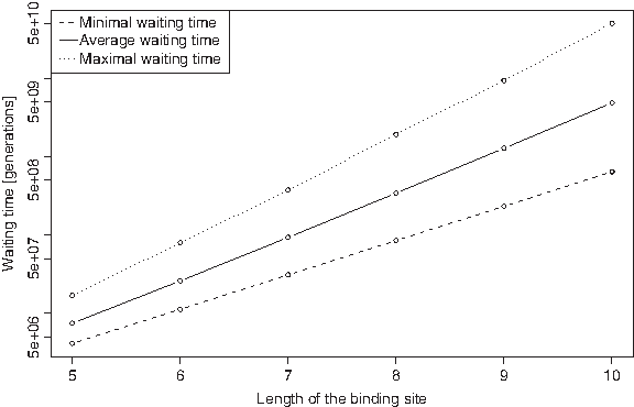
Minimal, maximal, and average waiting times in model M1 (log scale). These waiting times (generations) are computed based on the results in Table 2.

Let us focus on 5- and 10-mers. CCCTG is the fastest appearing 5-mer with an expected waiting time of 4,132,368 generations (≈83 Myrs) while ATATA is the slowest emerging 5-mer with a number of 16,906,864 generations (≈338 Myrs). This shows that incorporating the CpG methylation-deamination process into our model increases the variance in waiting times: on the one hand, the minimal waiting time for 5-mers in model M1 is much shorter than in model M0 (83 versus 126 Myrs) but, on the other hand, the maximal waiting time is much larger than in model M0 (338 versus 153 Myrs).

This variance is so high that for some (k + 1)-mers the waiting times are shorter than for some other k-mers. For example, the waiting time for the 5-mer ATATA is 338 Myrs and for the 6-mer CCCCTG it is only 224 Myrs. This confirms our approach of not just looking at waiting times in dependency of the length k of the TF binding site but also taking its composition into account. The effect gets even stronger for large k as can be seen in Figure 2: for small k, 5 ≤ k ≤ 7, the waiting times for k- and (k + 1)-mers are separated more clearly, for bigger k, 8 ≤ k ≤ 10, they overlap considerably.

FIG. 2.

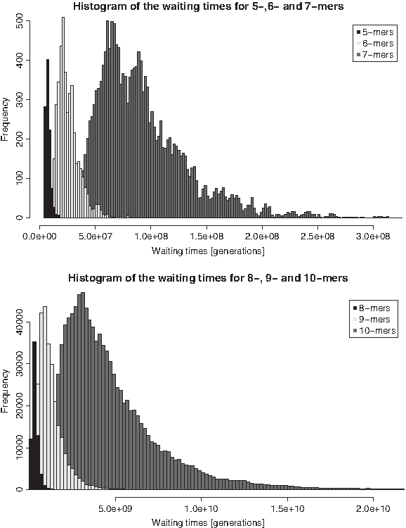
Histograms of the waiting times in model M1. The expected waiting times (generations) are taken from Table 2.

3.2.2. Waiting times for several promoters

The waiting times presented in the preceding section are quite long and by itself seem not to explain rapid evolutionary changes in regulatory regions. But answering the question how long one has to wait for one particular binding site to appear in one particular promoter may be too restrictive. Thus, we ask how long it takes until a new TF binding site emerges in at least one of all the human promoters. This could induce a change in gene regulation and hence, could be important for the evolution of the whole species (see Section 2.2.3). Assuming that there are around 20,000 human promoters, we computed the minimal, maximal and average waiting times \documentclass{aastex}\usepackage{amsbsy}\usepackage{amsfonts}\usepackage{amssymb}\usepackage{bm}\usepackage{mathrsfs}\usepackage{pifont}\usepackage{stmaryrd}\usepackage{textcomp}\usepackage{portland,xspace}\usepackage{amsmath,amsxtra}\pagestyle{empty}\DeclareMathSizes{10}{9}{7}{6} \begin{document}$${\mathbb E} ( T_m )$$\end{document} for k-mers to appear in at least one of m promoters, m ranging from 1 to 20,000. For k = 5 and k = 10, the results are depicted in Figure 3.

FIG. 3.

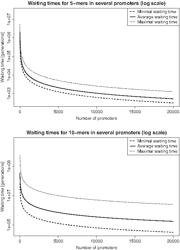
Waiting times in dependency of the number of promoters in model M1 (log scale). Minimal, maximal, and average waiting times (generations) for 5- and 10-mers to appear in at least one of several promoters.

The waiting times \documentclass{aastex}\usepackage{amsbsy}\usepackage{amsfonts}\usepackage{amssymb}\usepackage{bm}\usepackage{mathrsfs}\usepackage{pifont}\usepackage{stmaryrd}\usepackage{textcomp}\usepackage{portland,xspace}\usepackage{amsmath,amsxtra}\pagestyle{empty}\DeclareMathSizes{10}{9}{7}{6} \begin{document}$${\mathbb E} ( T_m )$$\end{document} decrease with m: \documentclass{aastex}\usepackage{amsbsy}\usepackage{amsfonts}\usepackage{amssymb}\usepackage{bm}\usepackage{mathrsfs}\usepackage{pifont}\usepackage{stmaryrd}\usepackage{textcomp}\usepackage{portland,xspace}\usepackage{amsmath,amsxtra}\pagestyle{empty}\DeclareMathSizes{10}{9}{7}{6} \begin{document} \begin{align*} { \mathbb E } ( T_m ) \approx { \cal O } \left( \frac { 1 } { m } \right). \tag{27} \end{align*}\end{document}

The expected waiting times for k-mers to be created in at least one of all 20,000 human promoters are shown in Table 3. For example, on average, it only takes 7,467 years for a 5-mer to emerge (minimally 4,142 years and maximally 16,917 years). For 8-mers, on average one has to wait 341,104 years - a time span far below the speciation time of e.g. human and chimp (Hobolth et al. (2007)). And for 10-mers, the average waiting time is 4.8 Myrs implying that in a time comparable to the human-chimp split, on average one expects a given TF binding site of length 10 to be created at random in at least one of all the human promoters. But even after 700,000 years some particular new TF binding sites of length 10 are expected to be created (e.g. CCCCCCCCCC, CCCCCCCCCA, CCCCCCCCTG).

Table 3.

Waiting Times for All Human Promoters in Model M1

	5-mers	6-mers	7-mers	8-mers	9-mers	10-mers
Min	4,142	11,232	30,930	84,711	231,477	640,977
Max	16,917	79,840	371,935	1,918,419	9,340,903	49,972,266
Average	7,467	25,903	92,911	341,104	1,274,206	4,824,591

Minimal, maximal, and average waiting times (years) for k-mers, 5 ≤ k ≤ 10, to appear in at least one of all human promoters.

3.2.3. Comparison with existing TF binding sites

Given lists of k-mers ranked according to their waiting time till emergence, we are interested if one can observe top ranking k-mers in existing TF binding sites. We downloaded the non-redundant JASPAR CORE database for vertebrates, Version 4, (Portales-Casamar et al., 2010) and extracted all the human TF binding site position count matrices (PCMs) of length k, 5 ≤ k ≤ 10, i.e., 37 PCMs. In order to compare PCMs with k-mers, we converted a given PCM into a set of k-mers via the following procedure: after having computed a maximal score of a PCM by summing over the maximal column entries, we set a threshold of 0.95 of the maximal score and extracted all 10-mers with a score above this threshold.

For example, in case of the SP1 binding site (Fig. 4), 273 is the maximal score (CCCCGCCCC), the score threshold is 260 and the resulting 10-mer set of putative SP1 binding sites is given by {CCCCACCCCC, CCCCCCCCCC, CCCCGCCCCC, CCCCTCCCCC}. This set contains the top ranking 10-mers, e.g. CCCCCCCCCC is even the number 1 top ranking 10-mer, i.e. the fastest emerging 10-mer (see Figures 2 and 4). We repeated this procedure for all the PCMs extracted from the JASPAR database, also including the reverse complement for every k-mer since the TF could also bind to the complementary DNA strand. To test if these observed k-mers are among the top ranking k-mers according to our model, we assigned the corresponding ranks to them (as illustrated in Figure 4) and normalized the ranks by dividing by 4 ^k in order to look at all k-mers simultaneously. The null hypothesis that the waiting times according to our model do not affect the appearance of real TF binding sites can then be formulated as \documentclass{aastex}\usepackage{amsbsy}\usepackage{amsfonts}\usepackage{amssymb}\usepackage{bm}\usepackage{mathrsfs}\usepackage{pifont}\usepackage{stmaryrd}\usepackage{textcomp}\usepackage{portland,xspace}\usepackage{amsmath,amsxtra}\pagestyle{empty}\DeclareMathSizes{10}{9}{7}{6} \begin{document} \begin{align*} \begin{split}H_0: \quad \hbox{the relative ranks assigned to the real TF binding sites stem from} \\ \hbox{a uniform distribution on } [ 0 , 1 ].\end{split} \tag{28} \end{align*}\end{document}

FIG. 4.

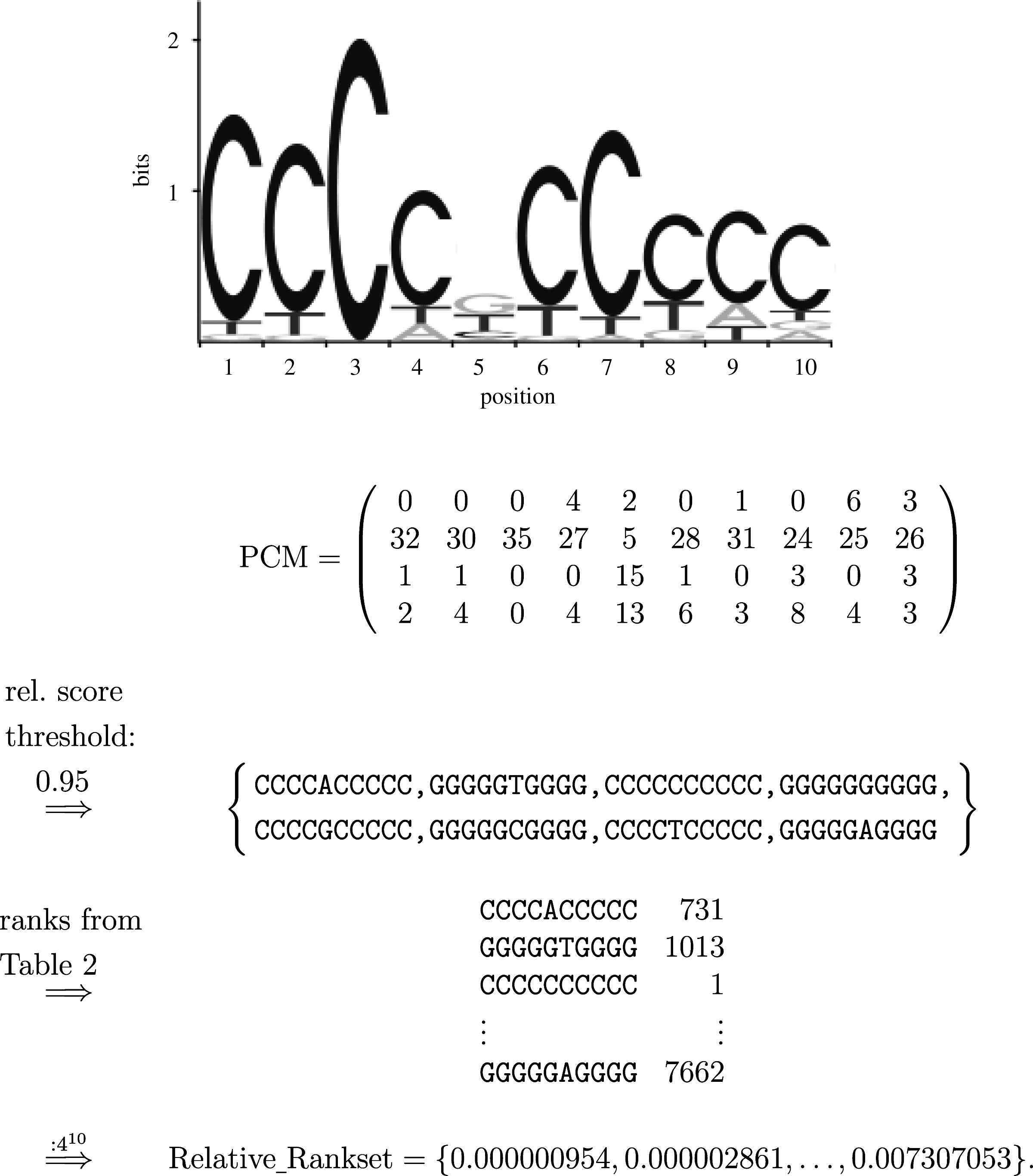
Example. Assuming that the SP1 motif is the set of 10-mers (and their reverse complements) with a score of at least 95% of the maximal score, we can derive the ranks for this 10-mer set, i.e., the ranks among all 10-mers in ascending order according to their waiting time until emergence and normalize them.

We performed Pearson's χ²-goodness-of-fit test yielding a p-value <2.2e − 16, i.e. one can reject the null hypothesis. The mean relative rank for the k-mers taken from JASPAR is 0.425 while the mean of the uniform distribution on [0, 1] is 0.5. Thus, k-mers with shorter waiting times are used more frequently as TF binding sites than other ones and as can be seen in Figure 5, a high proportion of existing TF binding sites belongs to the top ranking k-mers (around one quarter of them are among the top 10% ranks).

FIG. 5.

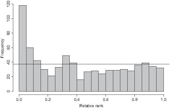
Histogram of the relative ranks of k-mers contained in JASPAR PCMs. For all JASPAR matrices of length k, 5 ≤ k ≤ 10, we assigned relative ranks to the k-mers with a relative score threshold of 0.95 (according to the procedure illustrated in Fig. 4). The horizontal line represents the uniform case, i.e., the case where the relative ranks would be distributed uniformly.

In this approach, for every TF, we have taken all of the possible k-mers (above a certain threshold) into account and thus, also included potentially slowly evolving k-mers. Hence, as a second step, we only looked at the rank of the fastest evolving binding site per TF. For every JASPAR TF we determined the k-mer with the smallest rank. Afterwards, we sorted all of the JASPAR TFs according to these minimal ranks. The results are depicted in Figure 6.

FIG. 6.

Histogram of the minimal relative ranks of JASPAR TFs. After having assigned relative ranks to the k-mers contained in JASPAR matrices (see Fig. 5), we determined the smallest relative rank for every TF. Thus, this figure depicts JASPAR TFs ranked according to their waiting time until appearance according to our model.

So under our model, the binding sites of the TFs SP1, TFAP2A, MZF1 5-13, REL, MZF1-4, NF-kappaB, RELA, ETS1, ELK1, BRCA1, SPIB and NFATC2 can be generated quickly while the appearance of binding sites like GATA2, FOXL1, MIZF and NKX3-1 binding sites requires long waiting times. Most of the TFs whose binding sites are predicted to be generated rapidly like BRCA1, NFKB, REL, RELA and SP1 are widely expressed and have been shown to interact with a lot of other proteins: e.g. BRCA1 has 225 interaction partners, REL 104, RELA 297, NFKB1 156, NFKB2 214 and SP1 has 156 interaction partners; numbers taken from the database UniHI (Chaurasia et al., 2007). In contrast, the binding sites of TFs which appear slowly according to our model are only expressed in certain tissues, e.g. the slowest evolving TF NKX3-1 is largely prostate and testis-specific, and have fewer interaction partners, e.g. NKX3-1 has 4, MIZF 11, FOXL1 30 and GATA2 21 interaction partners (numbers taken from UniHI).

4. Discussion

We have developed a probabilistic approach to study the evolution of regulatory regions allowing us to predict how long one has to wait for a given TF binding site of length k, k ranging from 5 to 10, to be created at random in the human species - either in one promoter of length 1 kb or in at least one of all the human promoters. Our results indicate that new TF binding sites can indeed appear on a small evolutionary time scale: for example, given that model M1 is an appropriate choice, on average around 7,500 years may be sufficient for a given 5-mer to emerge in at least one of all the human promoters, for 8-mers around 350,000 years and for 10-mers around 4.8 Myrs (model M1). But for some TF binding sites of length 10 like, for example, the SP1 binding site, a duration of 700,000 years may be enough. This reveals that new TF binding sites of length k, k ≤ 10, can easily appear in a time span significantly below or around e.g. the divergence time of human and chimp which is around 4 Myrs as stated by Hobolth et al. (2007).

According to our model, on average the expected waiting times increase exponentially with the length of the binding site. This suggests that in the evolution of primates, there should be a bias towards many short motifs instead of one long TF binding site in regulatory sequences. This is what one actually observes in eukaryotes; for example Wray et al. (2003) pointed out that promoters containing 10–50 binding sites for 5–15 different transcription factors are not uncommon. By computing the information content of eukaryotic TF binding sites, Wunderlich and Mirny (2009) found that in contrast to bacteria, single eukaryotic TF binding sites are too short and imprecise to guarantee specific binding which is compensated for by TF binding site clustering.

Furthermore, our results suggest that the composition of TF binding sites and not only their length play a crucial role concerning the waiting times for appearance: sometimes it is even more ”favorable” to wait for a particular (k + 1)-mer instead of waiting for another k-mer. For example, the waiting time for the 9-mer ACGTACGTA to appear in one of all promoters has been estimated to be around 1.3 Myrs and the one for the 10-mer CCCCCCCCCC to be only around 650,000 years. In consideration of the fastest and slowest emerging k-mers, one observes that k-mers containing products of the CpG methylation-deamination process (TG and CA) can rapidly appear in promoter sequences while TA- or CG-rich k-mers need a lot of time to be created at random. Hence, the CpG methylation-deamination process is probably a major determinant in generating new TF binding sites. It accelerates the emergence of some k-mers - which becomes obvious when comparing waiting times from the models M0 and M1. Simply assuming independently evolving nucleotides like Durrett and Schmidt (2007), Stone and Wray (2001), does not unveil the importance of this neighbor dependent substitution process for the creation of new TF binding sites. Thus, the more general model M1 should be preferred over the model M0.

We have tested whether our results are consistent with existing TF binding sites, i.e. if these TF binding sites are top ranking among all k-mers ranked in ascending order according to their waiting time till emergence. Based on PCMs from the database JASPAR (Portales-Casamar et al., 2010), we showed that this holds true for most of the cases. On the other hand, our model of predicting waiting times for the appearance of TF binding sites could be also used as a null model to detect TF binding sites which emerge slowly under the model but which are still observed. For example, the TATA-binding protein recognizes a motif containing TATA. But when looking at the waiting times in Table 2 (model M1), one surprisingly observes that k-mers containing TATA are among the slowest emerging k-mers. In this case, we speculate that due to the fact that the TATA-motif is probably one of the most crucial cis-regulatory elements, it ”has to” be quite rare and therefore ”should” not appear rapidly by the time passing to avoid drastic changes in gene regulation. Additionally, for future research it would be interesting to characterize the TFs with fast (resp. slowly) emerging binding sites with regard to biological properties (e.g. GO categories) similar to our approach in section 3.2.3. where we have examined the connection between the speed of binding site emergence and tissue-specificity/interaction partners. So far, we could observe that ubiquitous TFs are usually associated with fast emerging binding sites, while tissue-specific TFs are linked to slower emerging TF binding sites.

In summary, one can conclude that new TF binding sites are expected to emerge rapidly when taking all human promoter sequences as a basis. Apart from having computed the speed of de novo creation of k-mers, our approach now also reveals how the composition of a TF binding site as well as of the promoter sequence can influence the process of TF binding site emergence and therefore, extends the previous knowledge about the dynamics of promoter sequence evolution.