Markov Logic Networks in the Analysis of Genetic Data

Abstract

Abstract

Complex, non-additive genetic interactions are common and can be critical in determining phenotypes. Genome-wide association studies (GWAS) and similar statistical studies of linkage data, however, assume additive models of gene interactions in looking for genotype-phenotype associations. These statistical methods view the compound effects of multiple genes on a phenotype as a sum of influences of each gene and often miss a substantial part of the heritable effect. Such methods do not use any biological knowledge about underlying mechanisms. Modeling approaches from the artificial intelligence (AI) field that incorporate deterministic knowledge into models to perform statistical analysis can be applied to include prior knowledge in genetic analysis. We chose to use the most general such approach, Markov Logic Networks (MLNs), for combining deterministic knowledge with statistical analysis. Using simple, logistic regression-type MLNs we can replicate the results of traditional statistical methods, but we also show that we are able to go beyond finding independent markers linked to a phenotype by using joint inference without an independence assumption. The method is applied to genetic data on yeast sporulation, a complex phenotype with gene interactions. In addition to detecting all of the previously identified loci associated with sporulation, our method identifies four loci with smaller effects. Since their effect on sporulation is small, these four loci were not detected with methods that do not account for dependence between markers due to gene interactions. We show how gene interactions can be detected using more complex models, which can be used as a general framework for incorporating systems biology with genetics.

1. Introduction

Genome-wide association studies (GWAS) have allowed the detection of many genetic contributions to complex phenotypes in humans (see www.genome.gov). Studies of biological networks of different kinds, including genetic regulatory networks, protein-protein interaction networks and others, have made it clear, however, that gene interactions are abundant and are therefore of likely importance for genetic analysis (Manolio et al., 2009). Complex, non-additive interactions between genetic variations are very common and can potentially play a crucial role in determining phenotypes (Brem et al., 2005; Drees et al., 2005; Carter et al., 2007; Carter and Dudley, 2009). GWAS and similar statistical methods (such as classical QTL studies) generally assume additive models of gene interaction that attempt to capture a compound effect of multiple genes on a phenotype as a sum of partial influences of each individual gene (Hirschhorn and Daly, 2005; McCarthy et al., 2008). These statistical methods also assume no biological knowledge about the underlying processes or phenotypes. Since biological networks are complex, and since variations are numerous, unconstrained searches for associations between genotype and phenotype require large population samples, and can succeed only in detecting a limited range of effects. Without imposing any constraints based on biological knowledge searching for gene interactions is very challenging, particularly when input data consist of different data types coming from various sources.

The major question that motivated this work is “Can we constrain traditional statistical approaches by using biological knowledge to define some known networks that influence patterns in the data, and can such approaches produce more complete genetic models?” For example, we might use the patterns present in the genotype data to build more predictive models based on both genotype and phenotype data. Note that the problem of using biological knowledge to constrain a model of genetic interaction is closely connected to the problem of integrating various types of data in a single model. In this article, we employ a known artificial intelligence (AI) approach (i.e., Markov Logic Networks) to reformulate the problem of defining and finding genetic models in a general way and use it to facilitate detection of non-additive gene interactions. This approach allows us to lay the foundations for studies of essentially any kind of genetic model, which we demonstrate for a relatively simple model.

Markov Logic Networks (MLNs) are one of the most general approaches to statistical relational learning, a sub-field of machine learning, that combines two kinds of modeling: probabilistic graphical models, namely Markov Random Fields (MRFs), and first-order logic. Probabilistic graphical models, first proposed by Pearl (1988), offer a way to represent joint probability distributions of sets of random variables in a compact fashion. A graphical structure describing the probabilistic independence relationships in these models allows the development of numerous algorithms for learning and inference and makes these models a good choice for handling uncertainty and noise in data. On the other hand, first-order logic allows us to represent and perform inferences over complex, relational domains. Propositional (Boolean) logic, which biologists are most familiar with, describes the truth state on the level of specific instances, while first-order logic allows us to make assertions about the truth state of relations between subsets (classes) of instances. Moreover, using first-order logic we can represent recursive and potentially infinite structures such as Markov chains where a temporal dependency of the current state on the state at the previous time step can be instantiated to an infinite time series. Thus, first order logic is a very flexible choice for representing general knowledge, like that we encounter in biology.

MLNs merge probabilistic graphical models and first-order logic in a framework that gains the benefits of both representations. Most importantly, the logic component of MLNs provides an interface for adding biological knowledge to a model through a set of first-order constraints. At the same time, MLNs can be seen as a generalization of probabilistic graphical models since any distribution represented by the latter can be represented by the former, and this representation is more compact due to the first-order logic component. Even so, various learning and inference algorithms for probabilistic graphical models are applicable to MLNs and are thereby enhanced with logic inference.

One key advantage of logic-based probabilistic modeling methods, and in particular MLNs, is that they allow us to work easily with data that are not independent and identically distributed (not i.i.d.). Many statistical and machine learning methods assume that the input data is i.i.d., a very strong, and usually artificial, property that most biological problems do not share. For instance, biological variables most often have a spatial or temporal structure, or can even be explicitly described in a relational database with multiple interacting relations. MLNs thus provide a means for non-i.i.d. learning and joint inference of a model. While the input data used in GWAS and in other genetic studies are rich in complex statistical interdependencies between the data points, MLNs can easily deal with any of these data structures.

There are various modeling techniques that employ both probabilistic graphical models and first-order logic (Poole, 1993; Ngo and Haddawy, 1997; Glesner and Koller, 1995; Sato and Kameya, 1997; DeRaedt et al., 2007; Friedman et al., 1999; Kersting and DeRaedt, 2000; Pless et al., 2006; Richardson and Domingos, 2006). Many of them impose different restrictions on the underlying logical representation in order to be able to map the logical knowledge base to a graphical model. One common restriction employed (Sato and Kameya, 1997; DeRaedt et al., 2007; Kersting and DeRaedt, 2000; Pless et al., 2006) is to use only clausal first-order formulas of the form \documentclass{aastex}\usepackage{amsbsy}\usepackage{amsfonts}\usepackage{amssymb}\usepackage{bm}\usepackage{mathrsfs}\usepackage{pifont}\usepackage{stmaryrd}\usepackage{textcomp}\usepackage{portland,xspace}\usepackage{amsmath,amsxtra}\pagestyle{empty}\DeclareMathSizes{10}{9}{7}{6} \begin{document} $$ b_1 \wedge b_2 \wedge \ldots \wedge b_n \Rightarrow h $$ \end{document} that are used to represent cause-effect relationships. The majority of the methods (Ngo and Haddawy, 1997; Glesner and Koller, 1995; Kersting and DeRaedt, 2000) use Bayesian networks, directed graphical models, as the probabilistic representation. However, there are a few approaches (Pless et al., 2006; Richardson and Domingos, 2006) that instead use MRFs, undirected graphical models, to perform inferences.

We use MLNs (Richardson and Domingos, 2006) that merge unrestricted first-order logic with MRFs and, as a result, use the most general probabilistic logic-based modeling approach. In this article, we show this MLN-based approach to understanding complex systems and data sets. Similar to Yi et al. (2005), who proposed a Bayesian approach that can be used to infer models for QTL detection, our MLN-based approach is a model inference method that goes beyond just hypothesis testing. Moreover, in this article, we describe how we have adapted and applied MLN to genetic analysis so that complex biological knowledge can be included in the models. We have applied the method to a relatively simple genetic system and data set, the analysis of the genetics of sporulation efficiency in the budding yeast Saccharomyces cerevisiae. In this system, recently analyzed by Gerke et al. (2009), two genetically and phenotypically diverse yeast strains, whose genomes were fully characterized, were crossed and the progeny studied for the genetics of the sporulation phenotype. This provided a genetically complex phenotype with a well-defined genetic context to which to apply our method.

2. Methods

2.1. Markov random fields

Given a set of random variables of the same type, X = {X_i : 1 ≤ i ≤ N} and a set of possible values (alphabet) A = {A_i : 1 ≤ i ≤ M} so that any variable can take any value from A₁ to A_M (it is easy to extend this to the case of multiple variable types). Consider a graph, G, whose vertices represent variables, X, and whose edges represent probabilistic dependencies among the vertices such that a local Markov property is met. The local Markov property for a random variable X_i can be formally written as Pr(X_i = A_j|X \{X_i}) = Pr(X_i = A_j|N(X_i)) that states that a state of random variable X_i is conditionally independent of all other variables given X_i's neighbors N(X_i), N(X_i) ⊆ X\{X_i}. Let C denote the set of all cliques in G, where a clique is a subgraph that contains an edge for every pair of its nodes (a complete subgraph). Consider a configuration, γ, of X that assigns each variable, X_i, a value from A. We denote the space of all configurations as Γ = A^X. A restriction of γ to the variables of a specific clique C is denoted by γ _C .

A MRF is defined on X by a graph G and a set of potentials \documentclass{aastex}\usepackage{amsbsy}\usepackage{amsfonts}\usepackage{amssymb}\usepackage{bm}\usepackage{mathrsfs}\usepackage{pifont}\usepackage{stmaryrd}\usepackage{textcomp}\usepackage{portland,xspace}\usepackage{amsmath,amsxtra}\pagestyle{empty}\DeclareMathSizes{10}{9}{7}{6} \begin{document} $$ {\bf V} = \{V_C (\gamma_C) : C \in {\bf C} , \gamma \in {\bf \Gamma}\} $$ \end{document} assigned to the cliques of the graph. Using cliques allows us to explicitly define the topology of models, making MRFs convenient to model long-range, higher-order connections between variables. We encode the relationships between the variables using the clique potentials. By the Hammersley-Clifford theorem, a joint probability distribution represented by an MRF is given by the following Gibbs distribution \documentclass{aastex}\usepackage{amsbsy}\usepackage{amsfonts}\usepackage{amssymb}\usepackage{bm}\usepackage{mathrsfs}\usepackage{pifont}\usepackage{stmaryrd}\usepackage{textcomp}\usepackage{portland,xspace}\usepackage{amsmath,amsxtra}\pagestyle{empty}\DeclareMathSizes{10}{9}{7}{6} \begin{document} \begin{align*} {\rm Pr} (\gamma) = \frac {1} {Z} \prod_ {C \in {\bf C}} \exp (- V_C (\gamma_C)) , \tag {1} \end{align*} \end{document}

where the so-called partition function \documentclass{aastex}\usepackage{amsbsy}\usepackage{amsfonts}\usepackage{amssymb}\usepackage{bm}\usepackage{mathrsfs}\usepackage{pifont}\usepackage{stmaryrd}\usepackage{textcomp}\usepackage{portland,xspace}\usepackage{amsmath,amsxtra}\pagestyle{empty}\DeclareMathSizes{10}{9}{7}{6} \begin{document} $$ Z = \sum\nolimits_{\gamma \in {\bf \Gamma}} \prod\nolimits_{C \in {\bf C}} \exp (- V_C (\gamma_C)) $$ \end{document} normalizes the probability to ensure that \documentclass{aastex}\usepackage{amsbsy}\usepackage{amsfonts}\usepackage{amssymb}\usepackage{bm}\usepackage{mathrsfs}\usepackage{pifont}\usepackage{stmaryrd}\usepackage{textcomp}\usepackage{portland,xspace}\usepackage{amsmath,amsxtra}\pagestyle{empty}\DeclareMathSizes{10}{9}{7}{6} \begin{document} $$ \sum\nolimits_{\gamma \in {\bf \Gamma}} \Pr (\gamma) = 1 $$ \end{document} .

Without loss of generality, we can represent a MRF as a log-linear model (Pietra et al., 1997): \documentclass{aastex}\usepackage{amsbsy}\usepackage{amsfonts}\usepackage{amssymb}\usepackage{bm}\usepackage{mathrsfs}\usepackage{pifont}\usepackage{stmaryrd}\usepackage{textcomp}\usepackage{portland,xspace}\usepackage{amsmath,amsxtra}\pagestyle{empty}\DeclareMathSizes{10}{9}{7}{6} \begin{document} \begin{align*} {Pr} (\gamma) = \frac {1} {Z} \exp \left(\sum_i w_i f_i (\gamma)\right), \tag {2} \end{align*} \end{document}

where \documentclass{aastex}\usepackage{amsbsy}\usepackage{amsfonts}\usepackage{amssymb}\usepackage{bm}\usepackage{mathrsfs}\usepackage{pifont}\usepackage{stmaryrd}\usepackage{textcomp}\usepackage{portland,xspace}\usepackage{amsmath,amsxtra}\pagestyle{empty}\DeclareMathSizes{10}{9}{7}{6} \begin{document} $$ f_i: {\bf \Gamma} \rightarrow {\mathbb R} $$ \end{document} are functions defining features of the MRF and \documentclass{aastex}\usepackage{amsbsy}\usepackage{amsfonts}\usepackage{amssymb}\usepackage{bm}\usepackage{mathrsfs}\usepackage{pifont}\usepackage{stmaryrd}\usepackage{textcomp}\usepackage{portland,xspace}\usepackage{amsmath,amsxtra}\pagestyle{empty}\DeclareMathSizes{10}{9}{7}{6} \begin{document} $$ w_i \in {\mathbb R} $$ \end{document} are the weights of the MRF. Usually, the features are indicators of the presence or absence of some attribute, and hence are binary. For instance, we can consider a feature function that is 1 when some X_i has a particular value and 0 otherwise. Using these types of indicators, we can make M different features for X_i that can take on M different values. Given some configuration γ_X\{Xi} of all the variables X except X_i, we can have a different weight for this configuration whenever X_i has a different value. The weights for these features capture the affinity of the configuration γ_X\{Xi} for each value of X_i. Note that the functions defining features can overlap in arbitrary ways providing representational flexibility.

One simple mapping of a traditional MRF to a log-linear MRF is to use a single feature f_i for each configuration γ _C of every clique C with the weight w_i = −V_C(γ _C ). Even though in this representation the number of features (the number of configurations) increases exponentially as the size of cliques increases, the MLNs described in the next section attempt to reduce the number of features involved in the model specification by using logical functions of the cliques' configurations.

Given an MRF, a general problem is to find a configuration γ that maximizes the probability Pr(γ). Since the space Γ is very large, performing an exhaustive search is intractable. For many applications, there are two kinds of information available: (1) prior knowledge about the constraints imposed on the simultaneous configuration of connected variables; and (2) observations about these variables for a particular instance of the problem. The constraints constitute the model of the world and reflect statistical dependencies between values of the neighbors captured in an MRF. For example, when modeling gene association with phenotype, the restrictions on the likelihood of configurations of co-expressed genes may be cast as an MRF with cliques of size 2 and 3 (Fig. 1). In the next section, we give a biological example involving construction of MRFs with cliques of size 3 and 4, and provide more mathematical details. Fig. 1.

FIG. 1.

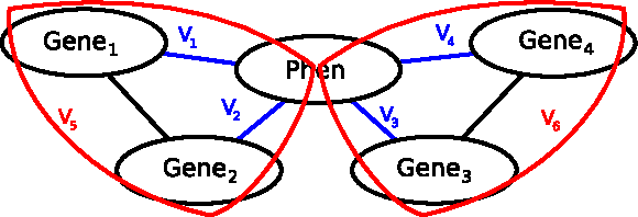
An example of a Markov Random Field: The MRF represents four genes influencing a phenotype with potentials \documentclass{aastex}\usepackage{amsbsy}\usepackage{amsfonts}\usepackage{amssymb}\usepackage{bm}\usepackage{mathrsfs}\usepackage{pifont}\usepackage{stmaryrd}\usepackage{textcomp}\usepackage{portland,xspace}\usepackage{amsmath,amsxtra}\pagestyle{empty}\DeclareMathSizes{10}{9}{7}{6} \begin{document} $$ V_1 , \ldots , V_4 $$ \end{document} (blue edges). This model restricts genetic interactions to two pair-wise interactions with potentials V₅,V₆ (red cliques).

2.2. Markov logic networks: mapping first-order logic to Markov random fields

MLNs merge MRFs with first-order logic. In first-order logic (FOL) we distinguish constants and variables that represent objects and their classes in a domain, as well as functions specifying mappings between subgroups of objects, and predicates representing relations among objects or their attributes. We call a predicate ground if all its variables are assigned specific values. To illustrate, consider a study of gene interactions through the phenotypic comparison of wild type strains, single mutants, and double mutants such as the one presented in Drees et al. (2005). Consider a set of constants representing genes, {g1,g2}, gene interaction labels, {A,B}, and difference between phenotype values of mutants, {0,1,2}. We define the following predicates: RelWS/2 (a 2-argument predicate which captures a relation between a wild type and a single mutant), RelWD/3 (a relation between a wild type and a double mutant), RelSS/3 (a relation between two single mutants), RelSD/4 (a relation between a single mutant and a double mutant), Int/3 (an interaction between two genes). Using FOL, we can define a knowledge base consisting of two formulas: \documentclass{aastex}\usepackage{amsbsy}\usepackage{amsfonts}\usepackage{amssymb}\usepackage{bm}\usepackage{mathrsfs}\usepackage{pifont}\usepackage{stmaryrd}\usepackage{textcomp}\usepackage{portland,xspace}\usepackage{amsmath,amsxtra}\pagestyle{empty}\DeclareMathSizes{10}{9}{7}{6} \begin{document} \begin{align*} \forall {\rm x , y} & \in \{ {\rm g}1 , {\rm g}2 \} , \forall {\rm c} \in \{ 0 , 1 \} , \forall {\rm v , u} \in \{ 0 , 1 , 2 \} , \\ & \qquad \qquad \qquad {\rm Int} ({\rm x , y , c}) \Rightarrow ({\rm RelWS} ({\rm x , v}) \Leftrightarrow {\rm RelSD} ({\rm y , x , y , u})) \\ \forall {\rm x , y} & \in \{{\rm g}1 , {\rm g}2 \} , \forall {\rm c} \in \{0 , 1\} , \forall {\rm v , u , w} \in \{0 , 1 , 2 \} , \\ & \qquad \qquad \qquad {\rm RelWS} ({\rm x , v}) \wedge {\rm RelWS} ({\rm y , u}) \wedge {\rm RelWD} ({\rm x , y , w}) \Rightarrow {\rm Int} ({\rm x , y , c}). \end{align*} \end{document}

The first rule represents the knowledge that depending on the type of interaction between two genes, there is a dependency between RelWS(x,v) and RelSD(y,x,y,u) relations. The second rule captures the knowledge that three relations, RelWS(x,v), RelWS(y,u), and RelWD(x,y,w), together determine the type of gene interaction.

Note that first-order formulas define relations between (potentially infinite) groups of objects or their attributes. Formulas in FOL can be seen as relational templates for constructing models in propositional logic. Therefore, FOL offers a compact way of representing and aggregating relational data. For example, two first-order formulas above can be replaced with 288 propositional formulas since variables x,y,c can be assigned 2 different values and variables u,v,w can be assigned 3 values. Moreover, using representational power of FOL, we can specify infinite structures such as temporal relations, e.g., Expression (e1,t1) ∧ NextTimeStep(t1, t2) ⇒ Expression(e2, t2), that can give rise to a theoretically infinite number of propositions.

The principal limitation of any strictly formal logic system is that it is not suitable for real applications where data contain uncertainty and noise. For example, the formulas specified earlier hold for the real data most of the time, but not always. If there is at least one data point where a formula does not hold, then the entire model is disregarded as being false. The two allowed states, true or false, is equivalent to allowing only probability values 1 or 0. MLNs, however, relax this constraint by allowing the model with unsatisfied formula with a lesser probability than one. The model with the smallest number of unsatisfied formulas will then be the most probable.

MLNs extend FOL by assigning a weight to each formula indicating its probabilistic strength. An MLN is a collection of first-order formulas F_i with associated weights w_i. For each variable of a MLN, there is a finite set of constants representing the domain of the variable. A MLN, together with its corresponding constants, is mapped to a MRF as follows.

Given a set of all predicates on an MLN, every ground predicate of the MLN corresponds to one random variable of a MRF whose value is 1 if the ground predicate is true and 0 otherwise. Similarly, every ground formula of F_i corresponds to one feature of the log-linear MRF whose value is 1 if the ground formula is true and 0 otherwise. The weight of the feature in the MRF is the weight w_i associated with the formula F_i in the MLN.

From the original definitions (1) and (2) and the fact that features of false ground formulas are equal to 0, the probability distribution represented by a ground MLN is given by \documentclass{aastex}\usepackage{amsbsy}\usepackage{amsfonts}\usepackage{amssymb}\usepackage{bm}\usepackage{mathrsfs}\usepackage{pifont}\usepackage{stmaryrd}\usepackage{textcomp}\usepackage{portland,xspace}\usepackage{amsmath,amsxtra}\pagestyle{empty}\DeclareMathSizes{10}{9}{7}{6} \begin{document} \begin{align*} {Pr} (\gamma) = \frac {1} {Z} \exp \left(\sum_i w_i n_i (\gamma) \right) = \frac {1} {Z} \prod_i \exp (- V_i (\gamma_i) n_i (\gamma)), \tag {3} \end{align*} \end{document}

where n_i(γ) is a number of true ground formulas of the formula F_i in the state γ (which directly corresponds to our data), γ _i is the configuration (state) of the ground predicates appearing in F_i. V _i is a potential function assigned to a clique which corresponds to F_i, and exp(−V _i (γ _i )) = exp(w_i). Note that this probability distribution would change if we changed the original set of constants. Thus, one can view MLNs as templates specifying classes of MRFs, just like FOL templates specifying propositional formulas.

Figure 2 illustrates a portion of a MRF corresponding to the ground MLN. We assume a set of constants and an MLN specified by the knowledge base from the example above, where a weight is assigned to each formula.

FIG. 2.

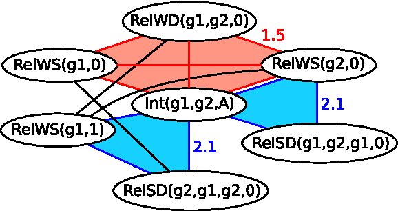
An example of a subnetwork of a Markov Random Field unfolded from a Markov Logic Network program: Each node of the MRF corresponds to a ground predicate (a predicate with variables substituted with constants). The nodes of all ground predicates that appear in a single formula form a clique such as the one highlighted with red. The blue triangular cliques correspond to the first formula of the MLN and are assigned the weight of the formula (2.1). The larger rectangular cliques, such as the one colored red, correspond to the second formula of the MLN with the weight 1.5.

2.3. An example: application to yeast sporulation dataset

We applied our method to a data set generated by Gerke et al. (2009). They generated and characterized a set of 374 progeny of a cross between two yeast strains that differ widely in their efficiency of sporulation (a wine and an oak strain). For each of the progeny the sporulation efficiency was measured and assigned a normalized real value between 0 and 1. To generate a discrete value set we then binned and mapped the sporulation efficiencies into 5 integer values. Each yeast progeny strain was genotyped at 225 markers that are uniformly distributed along the genome. Each marker takes on one of two possible values indicating whether it derived from the oak or wine parent genotype.

Using MLNs, we first model the effect of a single marker on the phenotype, i.e., sporulation efficiency. Define a logistic-regression type model with the following set of formulas: \documentclass{aastex}\usepackage{amsbsy}\usepackage{amsfonts}\usepackage{amssymb}\usepackage{bm}\usepackage{mathrsfs}\usepackage{pifont}\usepackage{stmaryrd}\usepackage{textcomp}\usepackage{portland,xspace}\usepackage{amsmath,amsxtra}\pagestyle{empty}\DeclareMathSizes{10}{9}{7}{6} \begin{document} \begin{align*} \forall {\rm strain} \in \{1 , \ldots , 374 \} , {\rm G} ({\rm strain , m , g}) \Rightarrow {\rm E} ({\rm strain , v}) , {\rm w}_{\rm m , g , v} , \tag{4} \end{align*} \end{document}

for every marker m under consideration (at this point we consider one marker in a model), genotype value \documentclass{aastex}\usepackage{amsbsy}\usepackage{amsfonts}\usepackage{amssymb}\usepackage{bm}\usepackage{mathrsfs}\usepackage{pifont}\usepackage{stmaryrd}\usepackage{textcomp}\usepackage{portland,xspace}\usepackage{amsmath,amsxtra}\pagestyle{empty}\DeclareMathSizes{10}{9}{7}{6} \begin{document} $$ {\rm g} \in \{{\rm A} , {\rm B}\} $$ \end{document} , and phenotype value \documentclass{aastex}\usepackage{amsbsy}\usepackage{amsfonts}\usepackage{amssymb}\usepackage{bm}\usepackage{mathrsfs}\usepackage{pifont}\usepackage{stmaryrd}\usepackage{textcomp}\usepackage{portland,xspace}\usepackage{amsmath,amsxtra}\pagestyle{empty}\DeclareMathSizes{10}{9}{7}{6} \begin{document} $$ {\rm v} \in \{{\rm 1} , \ldots , {\rm 5}\} $$ \end{document} . This MLN contains two predicates, G and E. Predicate G denotes markers' genotype values across yeast crosses, e.g., G(strain,M1,B) captures all yeast crosses for which the genotype of a marker M1 is B. Similarly, predicate E denotes the phenotype (sporulation efficiency) across yeast crosses, for instance, E(strain,1) captures all yeast strains for which the level of sporulation efficiency is 1. The MLN (4) contains 10 formulas, 1 marker of interest times 2 possible genotype values times 5 possible phenotype values. Each formula represents a pattern that holds true across all yeast crosses (indicated by the variable strain) with the same strength (indicated by the weight w_m,g,v). In other words, the weight w_m,g,v represents the fitness of the corresponding formula across all strains.

Instantiations of the predicate G represent a set of predictor variables, whereas instantiations of the predicate E represent a set of target variables (4). There are 748 ground predicates of G (assuming we handle only one marker in a model) and 1870 ground predicates of E. Each ground predicate corresponds to a random variable in the corresponding MRF (see the previous section for more details). Since our MLN contains 10 formulas and there are 374 possible instantiations for each formula, the corresponding log-linear MRF contains 3740 features, one for each instantiation of every formula.

2.4. Learning the weights of MLNs

Each data point in the original dataset corresponds to one ground predicate (either E or G in our example). For example, the information that a genotype value of a marker M71 in a strain S13 is equal to A corresponds to a ground predicate G(S13,M71,A). Therefore, the original dataset can be represented with a collection of ground predicates that logically hold, which in turn is described as a data vector \documentclass{aastex}\usepackage{amsbsy}\usepackage{amsfonts}\usepackage{amssymb}\usepackage{bm}\usepackage{mathrsfs}\usepackage{pifont}\usepackage{stmaryrd}\usepackage{textcomp}\usepackage{portland,xspace}\usepackage{amsmath,amsxtra}\pagestyle{empty}\DeclareMathSizes{10}{9}{7}{6} \begin{document} $$ {\bf d} = \langle d_1 , \ldots , d_N \rangle $$ \end{document} , where N is the number of all possible ground predicates (N = 2618 in this example). An element d_i of the vector d is equal to 1, if the ith ground predicate (assuming some order) is true and thus is included in our collection, and 0 otherwise. Note that this vector representation is possible under a closed world assumption stating that all ground predicates that are not listed in our collection are assumed to be false.

In order to carry out training of a MLN, we can use standard Newtonian methods for likelihood maximization. The learning proceeds by iteratively improving weights of the model. At the jth step, given weights w^(j), we compute \documentclass{aastex}\usepackage{amsbsy}\usepackage{amsfonts}\usepackage{amssymb}\usepackage{bm}\usepackage{mathrsfs}\usepackage{pifont}\usepackage{stmaryrd}\usepackage{textcomp}\usepackage{portland,xspace}\usepackage{amsmath,amsxtra}\pagestyle{empty}\DeclareMathSizes{10}{9}{7}{6} \begin{document} $$ \nabla_{{\bf w}^{(j)}} L ({\bf w}^{(j)}) $$ \end{document} , the gradient of the likelihood, which is our objective function that we maximize. Consequently, we improve the weights by moving in the direction of the positive gradient, \documentclass{aastex}\usepackage{amsbsy}\usepackage{amsfonts}\usepackage{amssymb}\usepackage{bm}\usepackage{mathrsfs}\usepackage{pifont}\usepackage{stmaryrd}\usepackage{textcomp}\usepackage{portland,xspace}\usepackage{amsmath,amsxtra}\pagestyle{empty}\DeclareMathSizes{10}{9}{7}{6} \begin{document} $$ {\bf w}^{(j + 1)} = {\bf w}^{(j)} + \alpha \nabla_{{\bf w}^{(j)}} L ({\bf w}^{(j)}) $$ \end{document} , where α is the step size.

Recall that the likelihood is given by \documentclass{aastex}\usepackage{amsbsy}\usepackage{amsfonts}\usepackage{amssymb}\usepackage{bm}\usepackage{mathrsfs}\usepackage{pifont}\usepackage{stmaryrd}\usepackage{textcomp}\usepackage{portland,xspace}\usepackage{amsmath,amsxtra}\pagestyle{empty}\DeclareMathSizes{10}{9}{7}{6} \begin{document} \begin{align*} L ({\bf w} \mid \gamma) = \Pr (\gamma \mid {\bf w}) = \frac {1} {Z} \exp \left(\sum_i w_i n_i (\gamma) \right) = \frac {\exp \left(\sum_i w_i n_i (\gamma) \right)} {\sum_ {\gamma^ {\prime} \in {\bf \Gamma}} \exp \left(\sum_i w_i n_i (\gamma^ {\prime}) \right)} , \tag {5} \end{align*} \end{document}

where γ is a state (also called a configuration) of the set of random variables X and Γ is a space of all possible states. Therefore, the log-likelihood is \documentclass{aastex}\usepackage{amsbsy}\usepackage{amsfonts}\usepackage{amssymb}\usepackage{bm}\usepackage{mathrsfs}\usepackage{pifont}\usepackage{stmaryrd}\usepackage{textcomp}\usepackage{portland,xspace}\usepackage{amsmath,amsxtra}\pagestyle{empty}\DeclareMathSizes{10}{9}{7}{6} \begin{document} \begin{align*} \log L ({\bf w} \mid \gamma) = \log \Pr (\gamma \mid {\bf w}) = \sum_i w_i n_i (\gamma) - \log \left[\sum_{\gamma^{\prime} \in {\bf \Gamma}} \exp \left(\sum_i w_i n_i (\gamma^{ \prime}) \right) \right]. \tag{6} \end{align*} \end{document}

Now derive the gradient with respect to the network weights, \documentclass{aastex}\usepackage{amsbsy}\usepackage{amsfonts}\usepackage{amssymb}\usepackage{bm}\usepackage{mathrsfs}\usepackage{pifont}\usepackage{stmaryrd}\usepackage{textcomp}\usepackage{portland,xspace}\usepackage{amsmath,amsxtra}\pagestyle{empty}\DeclareMathSizes{10}{9}{7}{6} \begin{document} \begin{align*} & \frac {\partial} {\partial w_j} \log L ({\bf w} \mid \gamma) = n_j (\gamma) - \frac {1} {\sum_ {\gamma^ {\prime} \in {\bf \Gamma}} \left[Z \Pr (\gamma^ {\prime}) \right]} \frac {\partial} {\partial w_j} \sum_ {\gamma^ {\prime} \in {\bf \Gamma}} \exp \left(\sum_i w_i n_i (\gamma^ {\prime}) \right) \\ & = n_j (\gamma) - \frac {1} {\sum_ {\gamma^ {\prime} \in {\bf \Gamma}} \left[Z \Pr (\gamma^ {\prime}) \right]} \sum_ {\gamma^ {\prime} \in {\bf \Gamma}} \left[n_j (\gamma^ {\prime}) \exp \left(\sum_i w_i n_i (\gamma^ {\prime}) \right) \right] & (7) \\ & = n_j (\gamma) - \sum_ {\gamma^ {\prime} \in {\bf \Gamma}} \left[n_i (\gamma^ {\prime}) L ({\bf w} \mid \gamma^ {\prime}) \right]. \end{align*} \end{document}

Note that the sum is computed over all possible variable states γ′. The above expression shows that each component of the gradient is a difference between the number of true instances a corresponding formula F_j (the number of true ground formulas of F_j) and the expected number of true instances of F_j according to the current model. However, computation of both components of the difference is intractably large.

Since the exact number of true ground formulas cannot be tractably computed from data (Richardson and Domingos, 2006), the number is approximated by sampling the instances of the formula and checking their truth values according to the data.

On the other hand, it is also intractable to compute the expected number of true ground formulas as well as the log-likelihood L(w|γ′). The former involves inference over the model, whereas the later requires computing the partition function \documentclass{aastex}\usepackage{amsbsy}\usepackage{amsfonts}\usepackage{amssymb}\usepackage{bm}\usepackage{mathrsfs}\usepackage{pifont}\usepackage{stmaryrd}\usepackage{textcomp}\usepackage{portland,xspace}\usepackage{amsmath,amsxtra}\pagestyle{empty}\DeclareMathSizes{10}{9}{7}{6} \begin{document} $$ Z = \sum\nolimits_{\gamma^{\prime} \in {\bf \Gamma}} \exp \left(\sum\nolimits_i w_i n_i (\gamma^{\prime})\right) $$ \end{document} . One solution, proposed in Richardson and Domingos (2006), is to maximize the pseudo-likelihood \documentclass{aastex}\usepackage{amsbsy}\usepackage{amsfonts}\usepackage{amssymb}\usepackage{bm}\usepackage{mathrsfs}\usepackage{pifont}\usepackage{stmaryrd}\usepackage{textcomp}\usepackage{portland,xspace}\usepackage{amsmath,amsxtra}\pagestyle{empty}\DeclareMathSizes{10}{9}{7}{6} \begin{document} \begin{align*} {\hat L} ({\bf w} \mid \gamma) = \prod_{j = 1}^N \Pr (\gamma_j \mid \gamma_{MB_j}; {\bf w}) , \tag{8} \end{align*} \end{document}

where γ _j is a restriction of the state γ to the jth ground predicate and γ _MBj is a restriction of γ to what is called a Markov blanket of the jth ground predicate (the state of the Markov blanket according to our data). We elected to use this approach. Similar to the original definition of the Markov blanket in the context of Bayesian networks (Pearl, 1988), the Markov blanket of a ground predicate is a set of other ground predicates that are present in some ground formula. Using the yeast sporulation example, the set of ground predicates { ∀ m, ∀ g | G(S1,m,g)} is the Markov blanket of E(S1,1) due to the knowledge base (4). Maximization of pseudo-likelihood is computationally more efficient than maximization of likelihood, since it does not involve inference over the model, and thus does not require marginalization over a large number of variables. Currently, we use the limited-memory Broyden-Fletcher-Goldfarb-Shanno (L-BFGS) algorithm from the Alchemy implementation of MLNs (Kok et al., 2007) to optimize the pseudo-likelihood.

2.5. Using MLNs for querying

After learning is complete, we have a trained MLN that can be used for various types of inference. In particular, we can answer such queries as “what is the probability that a ground predicate Q is true given that every predicate from a set (a conjunction) of ground predicates \documentclass{aastex}\usepackage{amsbsy}\usepackage{amsfonts}\usepackage{amssymb}\usepackage{bm}\usepackage{mathrsfs}\usepackage{pifont}\usepackage{stmaryrd}\usepackage{textcomp}\usepackage{portland,xspace}\usepackage{amsmath,amsxtra}\pagestyle{empty}\DeclareMathSizes{10}{9}{7}{6} \begin{document} $$ Ev = \{E_1 , \ldots , E_m\} $$ \end{document} is true?” The ground predicate Q is called a query and the set Ev is called an evidence. Answering this query is similar to computing the probability \documentclass{aastex}\usepackage{amsbsy}\usepackage{amsfonts}\usepackage{amssymb}\usepackage{bm}\usepackage{mathrsfs}\usepackage{pifont}\usepackage{stmaryrd}\usepackage{textcomp}\usepackage{portland,xspace}\usepackage{amsmath,amsxtra}\pagestyle{empty}\DeclareMathSizes{10}{9}{7}{6} \begin{document} $$ \Pr (Q \mid E_1 \wedge \ldots \wedge E_m , MLN) $$ \end{document} . Using the product rule for probabilities, we get \documentclass{aastex}\usepackage{amsbsy}\usepackage{amsfonts}\usepackage{amssymb}\usepackage{bm}\usepackage{mathrsfs}\usepackage{pifont}\usepackage{stmaryrd}\usepackage{textcomp}\usepackage{portland,xspace}\usepackage{amsmath,amsxtra}\pagestyle{empty}\DeclareMathSizes{10}{9}{7}{6} \begin{document} \begin{align*} &\Pr (Q \mid E_1 \wedge \ldots \wedge E_m , MLN) = \frac{\Pr (Q \wedge E_1 \wedge \ldots \wedge E_m \mid MLN)} {\Pr (E_1 \wedge \ldots \wedge E_m \mid MLN)} \\ &= \frac {\sum_ {\gamma \in {\bf \Gamma} _Q \cap {\bf \Gamma} _E} \Pr (\gamma \mid MLN)} {\sum_ {\gamma \in {\bf \Gamma} _E} \Pr (\gamma \mid MLN)} , \tag {9} \end{align*} \end{document}

where Γ _P is the set of all possible configurations where a ground predicate P is true, and \documentclass{aastex}\usepackage{amsbsy}\usepackage{amsfonts}\usepackage{amssymb}\usepackage{bm}\usepackage{mathrsfs}\usepackage{pifont}\usepackage{stmaryrd}\usepackage{textcomp}\usepackage{portland,xspace}\usepackage{amsmath,amsxtra}\pagestyle{empty}\DeclareMathSizes{10}{9}{7}{6} \begin{document} $$ {\bf \Gamma}_E = {\bf \Gamma}_{E_1} \cap \ldots \cap {\bf \Gamma}_{E_m} $$ \end{document} .

Computing the above probabilistic query for majority of real application problems, which include the computational problems posed by the complexity experienced in systems biology, is intractable. Therefore, we need to approximate \documentclass{aastex}\usepackage{amsbsy}\usepackage{amsfonts}\usepackage{amssymb}\usepackage{bm}\usepackage{mathrsfs}\usepackage{pifont}\usepackage{stmaryrd}\usepackage{textcomp}\usepackage{portland,xspace}\usepackage{amsmath,amsxtra}\pagestyle{empty}\DeclareMathSizes{10}{9}{7}{6} \begin{document} $$ \Pr (Q \mid E_1 \wedge \ldots \wedge E_m , MLN) $$ \end{document} , which can be done using various sampling-based algorithms.

MLNs adopt a knowledge-based model construction approach consisting of two steps: (1). constructing the smallest MRF from the original MLN that is sufficient for computing the probability of the query; and (2) inferring the MRF using traditional approaches. One of the commonly used inference algorithms is Gibbs sampling where at each step we sample a ground predicate X_j given its Markov blanket. In order to define the probability of the node X_j being in the state γ_j given the state of its Markov blanket we use the earlier notation.

Given a jth ground predicate X_j, all the formulas containing X_j are denoted by F _j . We denote the Markov blanket of X_j as MB_j and a restriction of γ to the Markov blanket (the state of the Markov blanket) as γ _MBj . Similarly, a restriction of the state γ to X_j is denoted as γ _j . Recall that each formula F of a MLN corresponds to a feature of a MRF, where the feature's value is the truth value f of the formula F depending on states \documentclass{aastex}\usepackage{amsbsy}\usepackage{amsfonts}\usepackage{amssymb}\usepackage{bm}\usepackage{mathrsfs}\usepackage{pifont}\usepackage{stmaryrd}\usepackage{textcomp}\usepackage{portland,xspace}\usepackage{amsmath,amsxtra}\pagestyle{empty}\DeclareMathSizes{10}{9}{7}{6} \begin{document} $$ \gamma_1 , \ldots , \gamma_k $$ \end{document} of the ground predicates \documentclass{aastex}\usepackage{amsbsy}\usepackage{amsfonts}\usepackage{amssymb}\usepackage{bm}\usepackage{mathrsfs}\usepackage{pifont}\usepackage{stmaryrd}\usepackage{textcomp}\usepackage{portland,xspace}\usepackage{amsmath,amsxtra}\pagestyle{empty}\DeclareMathSizes{10}{9}{7}{6} \begin{document} $$ X_1 , \ldots , X_k $$ \end{document} constituting the formula and denoted by \documentclass{aastex}\usepackage{amsbsy}\usepackage{amsfonts}\usepackage{amssymb}\usepackage{bm}\usepackage{mathrsfs}\usepackage{pifont}\usepackage{stmaryrd}\usepackage{textcomp}\usepackage{portland,xspace}\usepackage{amsmath,amsxtra}\pagestyle{empty}\DeclareMathSizes{10}{9}{7}{6} \begin{document} $$ f = F \mid _{\gamma_1 , \ldots , \gamma_k} $$ \end{document} . Note that \documentclass{aastex}\usepackage{amsbsy}\usepackage{amsfonts}\usepackage{amssymb}\usepackage{bm}\usepackage{mathrsfs}\usepackage{pifont}\usepackage{stmaryrd}\usepackage{textcomp}\usepackage{portland,xspace}\usepackage{amsmath,amsxtra}\pagestyle{empty}\DeclareMathSizes{10}{9}{7}{6} \begin{document} $$ F \mid _{\gamma_1 , \ldots , \gamma_k} $$ \end{document} can also be shown as \documentclass{aastex}\usepackage{amsbsy}\usepackage{amsfonts}\usepackage{amssymb}\usepackage{bm}\usepackage{mathrsfs}\usepackage{pifont}\usepackage{stmaryrd}\usepackage{textcomp}\usepackage{portland,xspace}\usepackage{amsmath,amsxtra}\pagestyle{empty}\DeclareMathSizes{10}{9}{7}{6} \begin{document} $$ F \mid _{\gamma_1 , \gamma_{MB_j}} $$ \end{document} . Using this notation we can express the probability of the node X_j to be in the state γ _j when its Markov blanket is in the state γ _MBj as \documentclass{aastex}\usepackage{amsbsy}\usepackage{amsfonts}\usepackage{amssymb}\usepackage{bm}\usepackage{mathrsfs}\usepackage{pifont}\usepackage{stmaryrd}\usepackage{textcomp}\usepackage{portland,xspace}\usepackage{amsmath,amsxtra}\pagestyle{empty}\DeclareMathSizes{10}{9}{7}{6} \begin{document} \begin{align*} \Pr (\gamma_j \mid \gamma_ {MB_j}) = \frac {\exp \left(\sum_{F_i \in {\bf F} _j} w_i F_i \mid _ {\gamma_j , \gamma_ {MB_j}} \right)} {\exp \left(\sum_ {t = 0} ^1 \sum_ {F_i \in {\bf F} _j} w_i F_i \mid _ {X_j = t , \gamma_ {MB_j}} \right)} . \tag {10} \end{align*} \end{document}

For the Gibbs sampling, we let a Markov chain converge and then estimate the probability of a conjunction of ground predicates to be true by counting the fraction of samples from the estimated distribution in which all the ground predicates hold. The Markov chain is run multiple times in order to handle situations when the distribution has multiple local maxima so that the Markov chain can avoid being trapped on one of the peaks. One of the current implementations, called Alchemy (Kok et al., 2007), attempts to reduce the burn-in time of the Gibbs sampler by applying a local search algorithm for the weighted satisfiability problem, called MaxWalkSat (Selman et al., 1993).

2.6. Components of the computational method

The general overview of the computational method is given in Figure 3. At the first step, the method traverses the set of all markers and assigns an error score to each marker indicating its predictive power. An error score of a marker corresponds to performance of an MLN (4) based on this single marker (a random variable m of (4) that essentially chooses the location of markers to use in the model has only one value the location of this single marker). The algorithm selects markers whose error scores are considerably lower than the average: we selected the outliers that are 3 standard deviations below the mean.

FIG. 3.

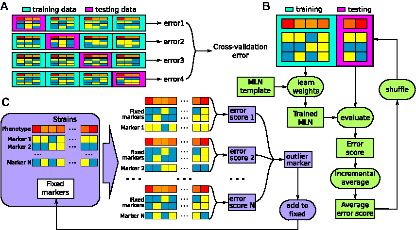
Components of the computational method: This figure illustrates three major computational components. We used cross-validation to estimate the goodness of fit of a model. (A) Four-fold cross-validation. The data is partitioned into four sets and at each iteration a model is trained on three sets and then tested on the fourth set resulting in four prediction error scores that are then averaged for a total cross-validation error. (B) Details of model training and testing. Using training data we estimate the weights of each formula of an MLN template. The trained MLN is evaluated on testing data resulting in an error score. We shuffle the order in the training data and the order of the testing data and repeat the training and testing. The error scores after each evaluation are averaged to produce the average error score of the MLN. (C) How the components illustrated in A and B are combined to search for the most informative markers. At the Nth iteration of the search, given a data set and set of N − 1 fixed markers, the method traverses the set of all markers and evaluates models constructed using the fixed markers and a selected marker. Note that at the Nth iteration, N-marker models consider the fixed markers (N − 1) as possible interactors with the next marker we found. The method then selects the outlier model, adds the corresponding marker to the set of fixed markers, and repeats the traversal of the markers. The method stops when no outliers are found.

The current version of the method greedily selects a marker with the lowest score and appends it to a list of fixed markers (which is initially empty). The algorithm then repeats the search for an outlier with the lowest score, but this time a marker's score is computed using an MLN (4) that estimates a joint effect of the marker under consideration together with all of the currently fixed markers on a phenotype (the variable m takes on the locations of all fixed markers and the marker under consideration). At each iteration, the algorithms expands the list of fixed markers and rescans all of the remaining markers for outliers. The method stops as soon as no more outliers are detected and returns the fixed markers as potential loci associated with the phenotype.

Our scanning for predictive genetic markers can be seen as an instance of the variable selection problem. We use cross-validation to compare probabilistic models and select the one with the best fit to the data and the smallest number of informative markers. Using cross-validation, we assess how a model generalizes to an independent dataset, addressing the model overfitting problem and facilitating unbiased outlier detection. Particularly, we use K-fold cross-validation which is illustrated in Figure 3A. The data set is arbitrarily split into K folds, \documentclass{aastex}\usepackage{amsbsy}\usepackage{amsfonts}\usepackage{amssymb}\usepackage{bm}\usepackage{mathrsfs}\usepackage{pifont}\usepackage{stmaryrd}\usepackage{textcomp}\usepackage{portland,xspace}\usepackage{amsmath,amsxtra}\pagestyle{empty}\DeclareMathSizes{10}{9}{7}{6} \begin{document} $$ {\bf D}_1 , \ldots , {\bf D}_K $$ \end{document} , and K iterations are performed. The ith iteration of cross-validation selects ∪ _j≠i D _j as a training dataset and D _i as a testing dataset. The model is then trained on the training dataset and the performance of the model is assessed using the testing dataset resulting in a prediction error. The average of prediction errors from K steps, called a cross-validation error, is used as a score of the model. In case of yeast sporulation efficiency dataset introduced earlier, we used 11-fold cross-validation (since a population of 374 yeast strains can be evenly partitioned into 11 subsets with 34 strains in each). The results were generally insensitive to the cross-validation parameters.

Recall that we distinguish two types of variables, the target variables whose values are predicted, and the predictor variables whose values are used to predict the values of the target variables. In the example above, sporulation efficiency of a yeast strain is a target variable, whereas genotype markers are predictor variables. Note that in some cases we can treat variables as both targets and predictors (e.g., gene expression in eQTL datasets). During the evaluation phase in the ith iteration of cross-validation, we consider the testing dataset D _i . Using knowledge-based model construction approach, we build a MRF that is small yet sufficient to infer the values of all target variables in the set D _i . The target variables are inferred based on the values of the predictor variables from D _i .

The model prediction of a target variable X that can take on any value from {x₁,x₂,x₃} can be represented as a vector \documentclass{aastex}\usepackage{amsbsy}\usepackage{amsfonts}\usepackage{amssymb}\usepackage{bm}\usepackage{mathrsfs}\usepackage{pifont}\usepackage{stmaryrd}\usepackage{textcomp}\usepackage{portland,xspace}\usepackage{amsmath,amsxtra}\pagestyle{empty}\DeclareMathSizes{10}{9}{7}{6} \begin{document} $$ {\hat{\bf v}} = < p_1 , p_2 , p_3 > $$ \end{document} , where p_j = Pr(X = x_j | D _i , Θ _MRF ) is the probability of X to take on a value x_j given the testing data D _i and the MRF with parameters Θ _MRF . On the other hand, the actual value of X (provided in the testing dataset D _i ) can be represented as a vector \documentclass{aastex}\usepackage{amsbsy}\usepackage{amsfonts}\usepackage{amssymb}\usepackage{bm}\usepackage{mathrsfs}\usepackage{pifont}\usepackage{stmaryrd}\usepackage{textcomp}\usepackage{portland,xspace}\usepackage{amsmath,amsxtra}\pagestyle{empty}\DeclareMathSizes{10}{9}{7}{6} \begin{document} $${\bf v} = < v_1, v_2, v_3 >$$ \end{document} , where ∀ j ≠ k,v_j = 0 and v_k = 1 iff X = x_k in D _i . Then the prediction error should measure the difference between the prediction \documentclass{aastex}\usepackage{amsbsy}\usepackage{amsfonts}\usepackage{amssymb}\usepackage{bm}\usepackage{mathrsfs}\usepackage{pifont}\usepackage{stmaryrd}\usepackage{textcomp}\usepackage{portland,xspace}\usepackage{amsmath,amsxtra}\pagestyle{empty}\DeclareMathSizes{10}{9}{7}{6} \begin{document} $$ {\hat {\bf v}} $$ \end{document} and the true value v. We used the Euclidean distance \documentclass{aastex}\usepackage{amsbsy}\usepackage{amsfonts}\usepackage{amssymb}\usepackage{bm}\usepackage{mathrsfs}\usepackage{pifont}\usepackage{stmaryrd}\usepackage{textcomp}\usepackage{portland,xspace}\usepackage{amsmath,amsxtra}\pagestyle{empty}\DeclareMathSizes{10}{9}{7}{6} \begin{document} $$ d ({\hat {\bf v}} , {\bf v}) $$ x \end{document} to compute the prediction error. This approach might make the comparison to other approaches difficult since the error can be a value that is not bounded by 0 and 1, but by 0 and \documentclass{aastex}\usepackage{amsbsy}\usepackage{amsfonts}\usepackage{amssymb}\usepackage{bm}\usepackage{mathrsfs}\usepackage{pifont}\usepackage{stmaryrd}\usepackage{textcomp}\usepackage{portland,xspace}\usepackage{amsmath,amsxtra}\pagestyle{empty}\DeclareMathSizes{10}{9}{7}{6} \begin{document} $$ {\sqrt M} $$ \end{document} , where M is the size of the domain of X (3 in our example). Further computation is required to obtain values for model accuracy, to explain variance, and other standard characteristics. On the other hand, Euclidean distance is certainly sufficient for comparing predictions of different models.

Due to the approximate nature of learning and inference in MLNs, two structurally identical models, trained on two data sets that differ only in the order of the samples, can generate predictions with slight differences. This is due to the fundamental path-dependency of learning and inference algorithms in knowledge-based model construction. For example, the order of training data affects the order in which the MRF is built, which in turn affects the way the approximate reasoning is performed over the field. Path-dependency introduces artificial noise into predictions and considerably reduces our ability to distinguish a signal with a small magnitude (such as a possible minor effect of a genetic locus on a phenotype) from a background.

In order to reduce the effect of path-dependency on overall model prediction we shuffle the input data set and average the resulting predictions. We employed an iterative approach, based on shuffling, for denoising. At each iteration, the model is retrained and reevaluated on newly shuffled data and the running mean of the model prediction is computed (Fig. 3B). The method incrementally computes the prediction average until achieving convergence, namely until the difference between the running average at the two consecutive iterations is smaller than Th for W consecutive steps. The parameters Th and W are directly connected with the total amount of shuffling and re-estimation performed as illustrated in Figure 4.

FIG. 4.

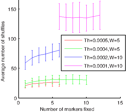
The amount of shuffling depends on the threshold and the size of the window: Note that the number of iterations until convergence of the algorithm increases when the threshold decreases or the window size increases. Note also that selecting tight stopping parameters tends to allow the algorithm to identify more informative markers.

In order to perform rigorous denoising, we select a lower value for the threshold Th (0.0001) and a larger window size W (10). The shuffling-based denoising procedure is applied at each iteration of the cross-validation. Averaging of the predictions after data shuffling reduces the amount of artificial noise enabling the overall method for detection of genetic loci to distinguish markers with a smaller effect on the phenotype (the algorithm detects more informative markers as illustrated in Figure 4).

There are many different strategies to search for the most informative subset of genetic markers. In this section, we used a greedy approach in order to illustrate the general MLN-based modeling framework presented in this article. In the next section we show that MLN-based modeling that accounts for dependencies between markers through joint-inference allows us to find interesting biological results by using a greedy search method. In order to be confident that the fixed markers are meaningful, we manually selected markers at each iteration of the search from the set of outliers and arrived at a similar set of candidate loci (within the same local region).

3. Results

The analyses presented in this article are based on the dataset from Gerke et al. (2009) containing both phenotype (sporulation efficiency) and genotype information of yeast strains derived from one intercross. The results are obtained using our method that searches for the largest set of genetic markers with the strongest compound effect on the phenotype. All the detailed information on the computational components of our method is presented in the Methods section.

In their article, Gerke et al. (2009) identified 5 markers that have an effect on sporulation efficiency including 2 markers whose effect seems to be very small. Moreover, Gerke et al. (2009) provided evidence for non-linear interactions between 3 major loci. The presence of confirmed markers with various effect and non-linear interactions make the dataset from Gerke et al. (2009) an ideal choice for testing our computational method.

Our method allows us to define and to use essentially any genetic model. First we used a simple regression-type model that mimics simple statisical approaches, like GWAS. At the first stage, the method compares the markers according to their individual predictive power. The amount of the effect of a marker on the phenotype is estimated by computing a prediction error score from a regression model based solely on this marker. The top line on the left panel in Figure 5 illustrates the error scores of all markers ordered by location (x-axis). In Figure 5, we observe three loci (around markers 71, 117, and 160) with the strongest effect on sporulation efficiency, which were identified in Gerke et al. (2009).

FIG. 5.

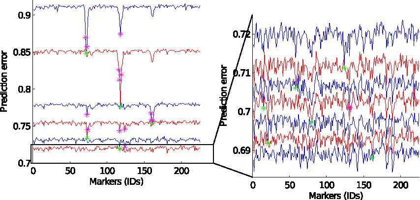
Prediction of sporulation efficiency using a subset of markers: This figure shows the execution of the algorithm plotted as error scores versus markers for a number of models. The top line in the left plot shows error scores of the models based only on a single marker plotted on the x-axis. A green star indicates the outlier marker with the smallest error and purple stars depict other outliers (markers whose error differs from the mean error by 3 standard deviations). The second line shows the error scores of the models based on a corresponding marker together with the previously selected marker (indicated with the green star). All the following lines are interpreted in the similar way. The left plot shows five markers with a large effect. The rest of the identified markers (six markers with a small effect) are illustrated in the right plot.

At the next stage, our method adds the marker with the strongest effect (marker 71) to all the following models. This allows us to compare all other markers according to their predictive power in conjunction with the fixed marker 71. This time the prediction error score of a marker indicates how well this marker together with the marker 71 predicts the sporulation efficiency. The score is, thus, computed from the regression model based on two markers: the marker 71 and a second marker. This is an important distinction from traditional GWAS where the searches for multiple influential markers are performed independently from each other. In our approach, using MLNs and in particular joint-inference, the compound effect of markers is estimated allowing us to see possible interactions between markers.

The method continues the iterations and selects 11 markers before the error no longer improves sufficiently and the computation stops. Among the selected markers, 5 are the same loci previously identified in Gerke et al. (2009) (markers 71, 117, 160, 123, 79), 3 are the markers next to the loci with the strongest effect (markers 72, 116, 161), and 3 are the new markers that have not been reported before (markers 57, 14, 20). In addition, the method identifies another marker (marker 130) as a candidate for a locus that has an effect on sporulation efficiency, although this marker was not selected due to its weak predictive power. Notice that even with a relatively simple model, such as logistic regression, and a quite stringent criterion for outliers (3 standard deviations from the mean, a p-value 0.003 for a normal distribution) we are able to exceed the number of identified candidate loci. We argue that our method is more efficient at discovering markers with a very low individual effect on phenotype that have non-trivial interactions with other sporulation-affecting loci due to the use of joint-inference of MLNs.

There are several distinct properties of our method that are important to note. First, although the method selects the neighboring markers of the three strongest loci, it does not select a neighbor immediately after the original loci has been identified, because there are better markers to be found. For example, after selecting the first marker 71, the method finds markers 117 and 160, and only then selects marker 72, which is the neighbor of 71. The method selects the next strongest marker at each stage that maximally increases the compound effect of selected markers. Second, our method does not find markers that do not add sufficient predictive power. The criterion for outliers determines when the method stops and determines the confidence that the added markers have a real effect on the phenotype.

For each new marker (57, 14, 20, 130) we examined all genes that were nearby (different actual distances were used). For example for the marker 14 we considered all genes located between markers 13 and 15. Table 1 shows genes located near these newly identified markers that are involved in either meiosis or in sporulation.

Table 1.

List of Genes Located Near the New Markers Identified by the MLN-Based Method

Marker	Euclidean error	Coord.	Candidate genes	GO	Description
57	0.7061	6, 103743	YFL039C, ACT1	S	Actin, structural protein involved in cell polarization, endocytosis, and other cytoskeletal functions
			YFL037W, TUB2	M	Beta-tubulin; associates with alpha-tubulin (Tub1p and Tub3p) to form tubulin dimer, which polymerizes to form microtubules
			YFL033C, RIM15	M	Glucose-repressible protein kinase involved in signal transduction during cell proliferation in response to nutrients, specifically the establishment of stationary phase; identified as a regulator of IME2; substrate of Pho80p-Pho85p kinase
			YFL029C, CAK1	M	Cyclin-dependent kinase-activating kinase required for passage through the cell cycle, phosphorylates and activates Cdc28p
			YFL009W, CDC4	M	F-box protein required for G1/S and G2/M transition, associates with Skp1p and Cdc53p to form a complex, SCFCdc4, which acts as ubiquitin-protein ligase directing ubiquitination of the phosphorylated CDK inhibitor Sic1p
			YFL005W, SEC4	S	Secretory vesicle-associated Rab GTPase essential for exocytosis
14	0.7009	2, 656824	YBR180W, DTR1	S	Putative dityrosine transporter, required for spore wall synthesis; expressed during sporulation; member of the major facilitator superfamily (DHA1 family) of multidrug resistance transporters
			YBR186W, PCH2	M	Nucleolar component of the pachytene checkpoint, which prevents chromosome segregation when recombination and chromosome synapsis are defective; also represses meiotic interhomolog recombination in the rDNA
130	0.7010	11, 447373	YKR029C, SET3	M	Defining member of the SET3 histone deacetylase complex which is a meiosis-specific repressor of sporulation genes; necessary for efficient transcription by RNAPII
			YKR031C, SPO14	S	Phospholipase D, catalyzes the hydrolysis of phosphatidylcholine, producing choline and phosphatidic acid; involved in Sec14p-independent secretion; required for meiosis and spore formation; differently regulated in secretion and meiosis
20	0.6972	3, 188782	YCR033W, SNT1	M	Subunit of the Set3C deacetylase complex that interacts directly with the Set3C subunit, Sif2p; putative DNA-binding protein

The table shows only the genes that are involved in sporulation or meiosis. Specific information for the genes can be found at www.yeastgenome.org.

The simple logistic regression-type model that was used can be summarized using the first-order formula G(strain,m,g) ⇒ E(strain,v), which captures the effect of a subset of markers on phenotype. In order to investigate gene-gene interactions we used a pair-wise model which can be summarized by the formula G(strain,m1,g1) ∧ G(strain,m2,g2) ⇒ E(strain,v). The pair-wise model subsumes the simple regression model, since whenever m1 and m2 are identical, the pair-wise MLN is mapped to the same set of cliques as those from the simple MLN. However, the pair-wise model defines the dependencies between two loci and a phenotype that are mapped to an additional set of 3-node cliques. The pair-wise model allows us explicitly to account for the pair-wise gene interactions. When using the pair-wise model, the joint-inference is performed over an MLN where possible interactions between two markers are specified with first-order formulas.

The assumption inherent in genome-wide analyses is that a simple additive effect can be observed when applying the pair-wise model to loci that do not interact: the compound effect is essentially a sum of the individual effects of each locus. On the other hand, for two interacting markers, the pair-wise model is expected to predict a larger-than-additive compound effect. Since the pair-wise model incorporates possible interactions, the prediction error of this model should be smaller than the error of a simple model by a factor that corresponds to how much the interaction information helps to improve the prediction.

By using the pair-wise model, we investigated the presence of interactions between markers 71, 117, 160 which correspond to loci with the strongest effect on sporulation efficiency. We denote the prediction error of a simple regression model based on markers \documentclass{aastex}\usepackage{amsbsy}\usepackage{amsfonts}\usepackage{amssymb}\usepackage{bm}\usepackage{mathrsfs}\usepackage{pifont}\usepackage{stmaryrd}\usepackage{textcomp}\usepackage{portland,xspace}\usepackage{amsmath,amsxtra}\pagestyle{empty}\DeclareMathSizes{10}{9}{7}{6} \begin{document} $$ M_1 , \ldots , M_n $$ \end{document} as \documentclass{aastex}\usepackage{amsbsy}\usepackage{amsfonts}\usepackage{amssymb}\usepackage{bm}\usepackage{mathrsfs}\usepackage{pifont}\usepackage{stmaryrd}\usepackage{textcomp}\usepackage{portland,xspace}\usepackage{amsmath,amsxtra}\pagestyle{empty}\DeclareMathSizes{10}{9}{7}{6} \begin{document} $$ error_S (M_1 , \ldots , M_n) $$ \end{document} , and the error of a pair-wise model based on markers \documentclass{aastex}\usepackage{amsbsy}\usepackage{amsfonts}\usepackage{amssymb}\usepackage{bm}\usepackage{mathrsfs}\usepackage{pifont}\usepackage{stmaryrd}\usepackage{textcomp}\usepackage{portland,xspace}\usepackage{amsmath,amsxtra}\pagestyle{empty}\DeclareMathSizes{10}{9}{7}{6} \begin{document} $$ M_1 , \ldots , M_n $$ \end{document} as \documentclass{aastex}\usepackage{amsbsy}\usepackage{amsfonts}\usepackage{amssymb}\usepackage{bm}\usepackage{mathrsfs}\usepackage{pifont}\usepackage{stmaryrd}\usepackage{textcomp}\usepackage{portland,xspace}\usepackage{amsmath,amsxtra}\pagestyle{empty}\DeclareMathSizes{10}{9}{7}{6} \begin{document} $$ error_{PW} (M_1 , \ldots , M_n) $$ \end{document} . Figure 6 compares the prediction errors of the simple regression model based on one marker (red line) and the errors of the pair-wise model based on two markers one of which is preset to 71 (blue line). Note that the baseline prediction error of the pair-wise model is the same as error_S(71), which means that on average the choice of a second marker in the pair-wise model does not affect the prediction. There are, however, 2 markers that visibly improve the prediction, namely markers 117 and 160. Note that the prediction error error_PW (71, 160) (the right blue peak) is lower than error_S(160) (the rightmost red peak) by only a value roughly equal to the difference between the average prediction errors of simple and pair-wise models (this value is equal to the size of the leftmost red peak). The reduction of the prediction error, when combining markers 71 and 160, is additive, suggesting that there is no interaction between these two markers. On the other hand, if we look at the effect of combining markers 71 and 117, we can see that the prediction improvement using the pair-wise model based on both markers (the size of the left blue peak) is considerably more than just a sum of prediction improvements of two simple models independently (the leftmost and the middle red peaks). The non-additive improvement suggests that there is an interaction between the markers 71 and 117.

FIG. 6.

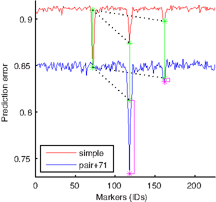
Investigating the 71–117 loci interaction: This figure compares a standard genome-wide scan made by a simple regression model based on a single marker (red line) and a scan made by a pair-wise model based on two markers, one of which is preset to 71 (blue line). The green lines represent the size of the leftmost red peak corresponding to the difference d between the baseline prediction error of the simple model and the error error_S(71). Pink bars represent how much the difference between error_S(117) and error_PW (71, 117) is larger than d. The large size of the leftmost pink bar indicates a strong interaction between markers 71 and 117.

Figures 7 and 8 show a similar analysis to that illustrated in Figure 6 performed on the other two markers. The analysis shown in Figure 7 confirms the interactions between markers 71 and 117 and, additionally, suggests that there is an interaction between markers 117 and 160. Figure 8 confirms the interaction between 117 and 160 and the absence of the interaction between 71 and 160. One can see from Figure 8 that the leftmost blue peak indicating error_PW (71, 160) is a sum of error_S(71) and error_S(160) (the pink bar next to the left pink star is extremely short). On the other hand, the rightmost blue peak is a lot more than just a sum of individual errors (the pink bar is tall). In fact, error_PW (117, 160) is almost the same as error_PW (71, 160).

FIG. 7.

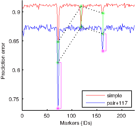
Investigation of 117–71 and 117–160 loci interactions: This figure compares a standard genome-wide scan using a single-marker model and a scan using a pair-wise model based on two markers, one of which is preset to 117. See the caption of Figure 6 for more details. Both pink bars indicate the presence of non-additive interactions between markers 117 and 71 and markers 117 and 160.

FIG. 8.

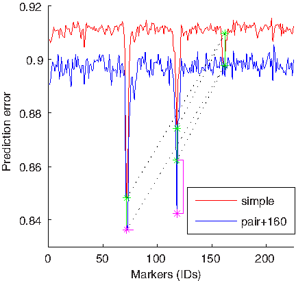
Investigating an interaction between markers 117 and 160: This figure compares a standard genome-wide scan using a single-marker model and a scan using a pair-wise model based on two markers, one of which is preset to 160. See the caption of Figure 6 for more details. Note error_PW (71, 160) that is almost the same as error_PW (117, 160) even though error_S(71) is considerably lower than error_S(117). The tall pink bar on the right side of the figure indicates a non-additive interaction between markers 117 and 160. On the other hand, the pink bar on the left is almost non-existent indicating absence of an interaction between markers 71 and 160.

The two predicted interactions, 71-117 and 117-160, were experimentally identified in Gerke et al. (2009). The strength of these interactions is significant enough to immediately stand out during the analysis in Figure 6. We next applied this analysis to the set of all nine identified loci (71, 117, 160, 123, 57, 14, 130, 79, 20) in order to quantify possible interactions between every pair of markers. For each two markers A and B from the set of loci, we compute the prediction errors of a simple model based solely on either A or B, denoted as error_S(A) and error_S(B). We also compute the prediction error of a pair-wise model based on both A and B, denoted as error_PW (A,B). Consequently, the size of a possible interaction between A and B, denoted as i(A,B), is estimated using the following expression: \documentclass{aastex}\usepackage{amsbsy}\usepackage{amsfonts}\usepackage{amssymb}\usepackage{bm}\usepackage{mathrsfs}\usepackage{pifont}\usepackage{stmaryrd}\usepackage{textcomp}\usepackage{portland,xspace}\usepackage{amsmath,amsxtra}\pagestyle{empty}\DeclareMathSizes{10}{9}{7}{6} \begin{document} \begin{align*} \begin{split} & i (A , B) = d (A , B) - d (A) - d (B) \\ & = (median - error_{PW} (A , B)) - (median - error_S (A)) - (median - error_S (B)) \\ & = error_S (A) + error_S (B) - error_{PW} (A , B) - median.\end{split} \tag{11} \end{align*} \end{document}

Here median is a baseline of prediction error of a simple model based on a single marker. We averaged the errors over 10 independently computed iterations. We next determined how high the value i(A,B) should be in order to confidently predict an interaction between markers A and B. We selected 36 pairs of randomly selected markers that were not from the set of nine informative markers and computed i(A, B) for each pair. Since we do not expect any interactions between random, non-informative markers, their i(A, B) values are used to estimate a confidence interval for no interaction. We computed a mean and standard deviation of the set of i(A, B) values corresponding to the randomly chosen markers. It is estimated that a value of 2.54 standard deviations away from the mean completely covers the set of i(A, B) values for all random markers, and we therefore argue there is a strong likelihood of interaction between markers A and B whenever i(A, B) is more than 3 standard deviations away from the mean. Whenever i(A, B) is less than 3 but more than 2.54 standard deviations away from the mean, we argue there is a probable interaction between A and B. Fig. 9. Estimated interactions between identified loci are illustrated as a network of marker interactions in Figure 9 where the color of each link represents the level of confidence of the corresponding interaction. We repeated the estimation of interactions by randomly selecting another 36 pairs of markers and computing the confidence intervals for the new set (2.32 standard deviations). The probable interactions identified from the first experiment were confirmed in the second experiment. Two possible interactions, however, were identified in one experiment but not the other and are depicted in Figure 9 with dashed links. This is a result of a slightly shifted mean of the second set of 36 random marker pairs relative to the first set, and the marginal size of the effect. Two interactions with very large i(A, B) values, 71–117 and 117–160, were previously identified in Gerke et al. (2009). We also found several smaller interactions illustrated in Figure 9 that have not been identified before. Note that since we measure absolute values i(A, B), it is not a surprise that interactions 71-117 and 117-160 are so large, since the corresponding loci (71, 117, 160) are by far the strongest. Locus 117, which is involved in the strongest interactions, corresponds to the gene IME1 (Gerke et al., 2009), the master regulator of meiosis (www.yeastgenome.com). Since IME1 is a very important sporulation gene, it is entirely reasonable that this gene is central to our interaction network (Fig. 9).

FIG. 9.

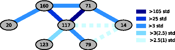
Estimated network of gene-gene interactions: This figure shows a network of estimated interactions between loci based on genetic data and sporulation phenotype. The color of the links corresponds to the level of confidence of interactions. The three darkest colors are associated with the most likely interactions. The fourth color is associated with an interaction 123–117 that scored high in the first experiment (more than 3 standard deviations away from the mean), but lower in the second experiment (2.5 standard deviations), although still above the confidence level (2.32 standard deviations). Two possible interactions depicted with the dashed lines with the lightest color scored above the confidence level in the first experiment (2.54 standard deviations), but below the confidence level in the second experiment (1 standard deviation). Loci 160, 71, 117, 123, 79 were previously identified in Gerke et al. (2009). Moreover, the genes of the three major loci were detected: IME1 (locus 117), RME1 (locus 71), and RSF1 (locus 160) (Gerke et al., 2009). The two strongest interactions, 160-117 and 117–71, were also identified in Gerke et al. (2009).

4. Discussion

The method presented in this article provides a framework for using virtually any genetic model in a genome-wide study because of the high representational power of MLNs. This power stems from the use of general, FOL conjoined to probabilistic reasoning. Moreover, the use of knowledge-based model approaches that build models based on both data and a relevant set of first order formulas (Wellman et al., 1992) allows us to efficiently incorporate prior biological knowledge into a genetic study. The generality of MLNs allows greater representational power than most modeling approaches. The general approach can be viewed as a seamless unification of statistical analysis, model learning and hypothesis testing.

As opposed to standard genome-wide approaches to genetics which assume additivity, the aim of the method described in this article is not to return values corresponding to the strength of individual effects of each marker. Our method aims at discovering the loci that are involved in determining the phenotype. The method computes the error scores for each marker in the context of the others representing the strength of each marker's effect in combination with other markers. It will be valuable in future to derive a scoring technique for markers that can be used directly to compare with results of the traditional approaches. In general, our approach provides a way of searching for the best model predicting the phenotype from the genetic loci. Since the model and the corresponding joint-inference methodology incorporate the relations between the model variables, we are able to begin a quantitative exploration of possible interactions between genetic loci.

Our method shows promise in that it can accommodate complex models with internal relationships among the variables specified. The development of a succinct and clear language, and grammar based on FOL for the description of (probabilistic) biological systems knowledge will be critical for the widespread application of this method to genetic analyses. Achieving this goal will also represent a significant step toward the fundamental integration of systems biology and the analysis and modeling of networks with genetics. Additionally, the development of the biological language describing useful biological constraints can alleviate the computational burden associated with model inference. MLN-based methods, such as ours, that perform both logic and probabilistic inferences are computationally expensive. While increases in computing power steadily reduce the magnitude of this problem, there are other approaches that will be necessary. Given such a focused biological language, we could tailor the learning and inference algorithms specifically to our needs and thus reduce the overall computational complexity of the method. Another future direction will be to find fruitful connections between a previously developed information theory-based approach to gene interactions (Carter et al. 2009) with this AI-derived approach. There are clear several other applications of this approach in the field of biology. It is clear that there are, for example, many similarities between the problem discussed here and the problems of data integration.

Biomarker identification, particularly for panels of biomarkers, is another important problem that involves many challenges of data integration and that can benefit from our MLN-based approach. Similar to GWAS or QTL mapping, where we search for genetic loci that are linked with a phenotype of interest, in biomarker detection we search for proteins or miRNAs that are associated with a disease state in a set of patient data. Just as in genetics, we can represent biomarkers as a network because there are various underlying biological mechanisms that govern the development of a disease. Often, the most informative markers from a medical point of view have weak signals by themselves. MLNs can allow us to incorporate partial knowledge about the underlying biological processes to account for the inter-dependencies making the detection of the informative biomarkers more effective. It is clear that the approach described here has the potential to integrate the biomarker problem with human genetics, a key problem in the future development of personalized medicine.