Sage Journals: Discover world-class research

Abstract

Introduction:

One manipulation used to study the neural basis of working memory (WM) is to vary the information load at encoding, then measure activity and connectivity during maintenance in the delay period. A hallmark finding is increased delay activity and connectivity between frontoparietal brain regions with increased load. Most WM studies, however, employ simple stimuli during encoding and unfilled intervals during the delay. In this study, we asked how delay period activity and connectivity change during low and high load maintenance of complex stimuli.

Methods:

Twenty-two participants completed a modified Sternberg WM task with two or five naturalistic scenes as stimuli during scalp electroencephalography (EEG). On each trial, the delay was filled with phase-scrambled scenes to provide a visual perceptual control with similar color and spatial frequency as presented during encoding. Functional connectivity during the delay was assessed by the phase-locking value (PLV).

Results:

Results showed reduced theta/alpha delay activity amplitude during high compared with low WM load across frontal, central, and parietal sources. A network with higher connectivity during low load consisted of increased PLV between (1) left frontal and right posterior temporal sources in the theta/alpha bands, (2) right anterior temporal and left central sources in the alpha and lower beta bands, and (3) left anterior temporal and posterior temporal sources in the theta, alpha, and lower beta bands.

Discussion:

The findings suggest a role for interhemispheric connectivity during WM maintenance of complex stimuli with load modulation when limited attentional resources are essential for filtering.

Impact statement

The patterns of brain connectivity subserving working memory (WM) have largely been investigated to date using simple stimuli, including letters, digits, and shapes and during unfilled WM delay intervals. Fewer studies describe functional connectivity changes during the maintenance of more naturalistic stimuli in the presence of distractors. In the present study, we employed a scene-based WM task during electroencephalography in healthy humans and found that during low-load WM maintenance with distractors increased interhemispheric connectivity in frontotemporal networks. These findings suggest a role for increased interhemispheric connectivity during maintenance of complex stimuli when attentional resources are essential for filtering.

Introduction

Previous functional magnetic resonance imaging (fMRI) (Bollinger et al., 2010; Hampson et al., 2006), electroencephalography (EEG) (Babiloni et al., 2004; Palva et al., 2010), and primate single-unit research (Constantinidis et al., 2018; Kamiński and Rutishauser, 2020; Sreenivasan et al., 2014) support that maintenance of information in working memory (WM) depends on activity within a frontoparietal network.

More recently an activity-silent account of WM posits that rapid changes in synaptic weights during the encoding of stimuli support maintenance making it possible to hold online unattended stimuli during a delay period without the need for persistent or transient activity (Beukers et al., 2021; Kamiński and Rutishauser, 2020; Stokes, 2015). In this view, maintenance is carried out by connectivity changes (Babiloni et al., 2004; Gazzaley et al., 2004; Hampson et al., 2006) induced by altered synaptic strengths while storage of information remains activity silent (Kamiński and Rutishauser, 2020; Stokes et al., 2020).

While findings implicate activity and connectivity as neural candidates for WM maintenance, a gap in knowledge exists since most studies of WM utilize simple stimuli at encoding (e.g., shapes or letters) followed by unfilled delay periods (blank screens with center fixation crosshairs). Simple stimuli have historically been used to reduce trial-to-trial variability and to control for novelty, but limitations to using simple stimuli include that they are highly familiar and not ecologically representative.

Complex stimuli increase the amount of information that must be maintained in WM (Alvarez and Cavanagh, 2004; Awh et al., 2007), which likely recruits brain regions in addition to the frontoparietal circuit typically recruited during maintenance, places greater demands on attention than simple shapes because they have more features to be combined for perception (Lavie et al., 2004), and requires more executive resources to maintain stimuli as well as filter irrelevant information that could interfere with maintenance (Lavie, 1995).

The use of unfilled delay periods has historically predominated in WM studies because they allow for a clear distinction of delay-related activity from background activity that is uncontaminated by perceptual or distractor noise. With unfilled delays, attention is assumed to be fully engaged and reflected by sustained activity in prefrontal and parietal cortex (Constantinidis et al., 2018; Goldman-Rakic, 1995; Sreenivasan et al., 2014).

Increased alpha power and event-related synchronization measured with EEG have also been identified as correlates of verbal WM maintenance during delay periods in posterior temporoparietal (Feredoes et al., 2011; Sarnthein et al., 1998; Scheeringa et al., 2009) and superior parietal regions (Jensen et al., 2002; Palva et al., 2010) as well as visual WM maintenance (Heinz and Johnson, 2017; Tuladhar et al., 2007). These patterns likely reflect suppression of potentially interfering neural processes (Jensen and Mazaheri, 2010) to minimize external distraction (Bonnefond and Jensen, 2012).

In the absence of visual stimuli during the delay period, increases in theta (Jensen and Tesche, 2002) and beta band activity (Jensen and Mazaheri, 2010) in frontal regions have been observed, potentially reflecting engagement of attentional processes and control during stimulus maintenance. In addition to increased activity during the delay period, increased connectivity in lower frequency bands, including theta and alpha have been attributed to attentional processes (Palva et al., 2010; Zhang et al., 2016), whereas higher bands like beta and gamma have been attributed to stimulus representation (Palva et al., 2010).

Taken together, there is a need to understand whether persistent neural activity or connectivity changes support the maintenance of complex stimuli at increasing WM load during delay periods filled with perceptually similar distractors.

The goal of the present study was to identify whether persistent neural activity patterns support WM maintenance for complex visual stimuli or whether connectivity changes support maintenance in the absence of persistent activity. The hypothesis is that introducing perceptually similar visual information during the delay period will engage attention and distract from maintenance, and it is predicted that the introduction of interference will be reflected in transient delay activity and reduced connectivity in lower frequency ranges. When there is a greater demand on attentional resources, at higher WM load, there are fewer resources available to process the interfering stimuli, and consequently functional connectivity will be reduced in the lower frequency bands compared with a low-load condition.

A low-load WM condition requires fewer attentional resources, so there will be more resources available to deal with interfering stimuli presented during the delay, so it is predicted that performance will be better at low load and consequently there will be increased connectivity in lower frequency bands during the delay period to support filtering of interference. Additionally, delay activity will be persistent and performance will be better, representing more successful storage than at high load.

Methods

Participants

The protocol was approved by the Institutional Review Board of The City University of New York Human Research Protection Program with procedures carried out according to the relevant guidelines and regulations. The study included 22 subjects (12 females, 18–54 years of age, mean age 24.95 years, standard deviation [SD] = 8.57).

Memory tasks

This study employed a variant of Sternberg WM task (Sternberg, 1966) with low (two stimuli) and high (five stimuli) loads. Participants completed 50 trials of each load. Loads were presented in randomized order (i.e., participant 1: low-load first, high-load second; participant 2: high-load first, low-load second, etc.). Participants completed three practice trials for each condition before recordings were begun.

Each WM task consisted of an encoding phase (with 2 or 5 stimuli each presented for 1400 msec each, Fig. 1), a delay period (6000 msec), a yes/no 50/50 probe choice (1400 msec) followed by jitter (∼3000 msec) consisting of a blank screen. During the delay period, six phase-scrambled scenes were presented each for 1000 msec. Phase scrambling preserves color and spatial frequency information but removes semantic content, which allows for them to serve both as a perceptual baseline relative to the encoding condition and as distractor stimuli relative to a static blank screen with fixation cross.

FIG. 1.

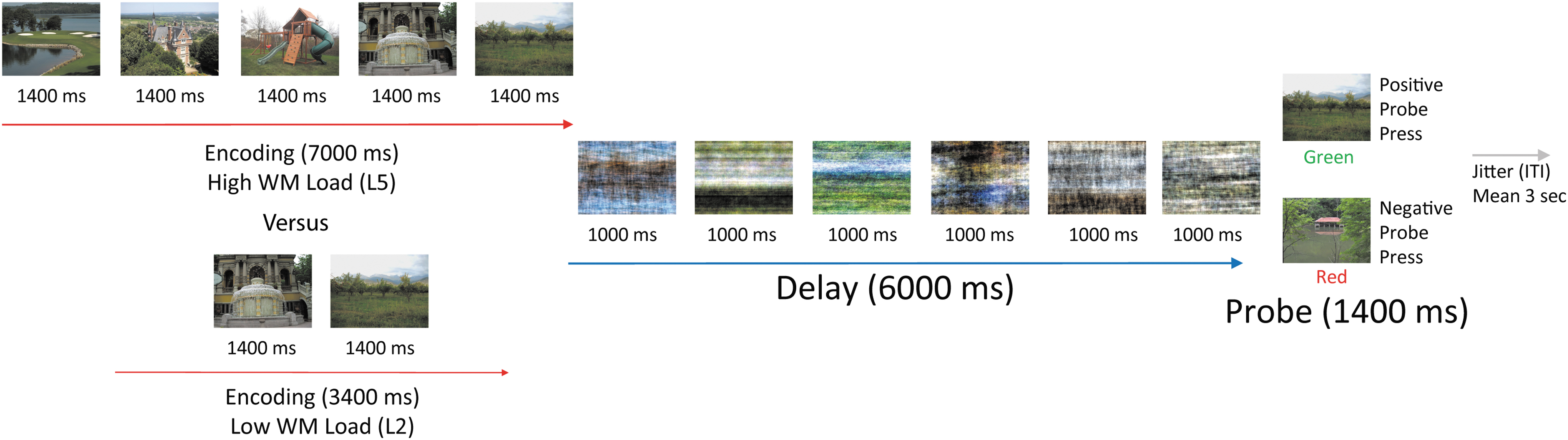
High- and low-load WM task trial layout. The task consisted of two WM loads: a low load (two scene stimuli) and a high load (five stimuli). In the high-load condition (top): participants were presented with five images in succession (1.4 sec each), a delay period with six phase-scrambled images (1 sec per image for a total delay period duration of 6 sec), a probe choice (1.4 sec), which was either one of the earlier presented stimuli or a new image, and a jitter period (∼3 sec) with a blank gray screen that indicates the end of the trial. For the low-load condition (bottom): participants were presented with two images in succession (1.4 sec each), a delay period with 6 phase-scrambled images (1 sec per image for a delay period total of 6 sec), a probe choice (1.4 sec), which is either one of the earlier presented images or a new image, and a jitter period (∼3 sec) with a blank gray screen that signaled the end of the trial. Participants completed both loads in randomized order. WM, working memory.

Participants were instructed to look at but not remember the phase-scrambled stimuli during the delay while maintaining the scene stimuli presented during the encoding phase. Evidence that these phase-scrambled stimuli served as interference during the delay comes from the detrimental effects on memory found in a separate behavioral study that we conducted before this EEG study (see Supplementary Data S1).

For the probe choice task, participants were presented with either a new scene (negative probe) or a previously presented old scene (positive probe), after which they had to signal by button press if they saw the scene before or not. Participants responded using a fiber optic response pad (Current Designs, Inc., Philadelphia, PA, USA) that they held in their right hand. They pressed a green button on the left of the pad for “Yes” and a red button on the right for “No.”

Scene stimuli were color outdoor naturalistic scenes from the SUN database (Xiao et al., 2010), 800 by 600 pixels and displayed on a gray background. Stimuli were randomly presented within each trial using an BOLDscreen LCD monitor that was located behind the MRI bore. Participants viewed the monitor in a mirror above them attached to the head coil. Before beginning the task, the experimenters confirmed that participants were able to see the monitor clearly. During the experimental session, participants were not able to see the button box. They were asked to memorize the location of the green and red buttons and to press the red and green buttons separately to confirm they knew the correct yes/no button mapping before beginning the task.

EEG acquisition

We collected continuous 32-channel EEG from passive electrodes (31-scalp electrodes and one electrocardiography [ECG] electrode) inserted in Brain Vision MR-safe caps while simultaneously acquiring structural and fMRI. One subject had EEG recorded from 64 channels (63-scalp and 1 ECG electrode), but for comparison with the other participants a 32-channel montage was applied to process this participant's data. This subject was included in all EEG analyses, except for the connectivity analysis described below because a custom source montage was not available.

Scalp electrodes were arranged according to the 10-10 International System. According to Brain Products simultaneous EEG–fMRI acquisition guidelines (Brain Products BrainAmp MR Operating and Reference manual Version 4.0), AgAL MR-safe gel was used to bring all electrode impedances to 20 kOhm or below. An ECG electrode was placed on the back left shoulder blade to record ballistocardiogram (BCG).

EEG caps were prepared and fitted outside the scanner and impedances were checked again after positioning on the scanner bed and movement into the bore. For safety, impedances were monitored throughout the scanning session. If impedances exceeded 35 kOhm between scans, the participant was removed from the bore, and more gel was applied until the impedance was lowered. After adjustments, the participant was repositioned and returned to the bore and impedances were checked again before repeating a localizer scan and continuing with recording.

EEG data were recorded at 2500 Hz. Each participant was positioned 40 mm caudal to isocenter in the bore of the 3.0 Tesla Siemens scanner (Mullinger et al., 2011). Initially, the first few subjects (n = 5) were recorded at 500 or 1000 Hz and sample rate was increased to 2500 Hz to improve fMRI artifact cleaning. Changes in sampling rate were based on manufacturer recommendations during experimental start-up. After fMRI artifact cleaning was completed, data from all participants were downsampled to 500 Hz.

EEG processing

EEG processing was done using BESA Research 7.0. MRI artifact correction was carried out using the BESA Research fMRI artifact gradient removal algorithm with the Allen Method (Allen et al., 2000) following the default BESA settings (number of artifact occurrence averages = 16). This method includes a sliding-window template with eight artifact occurrences before and after the artifact to create the artifact template, which is then subtracted from the data. The duration of each fMRI volume was automatically detected (repetition time = 2000 msec) and was based on the user-defined fMRI trigger code (R128) recorded during the session, which appeared after the initial three dummy scans.

For the first 19 participants, the fMRI trigger code was not recorded in the EEG files and was instead substituted by a trigger code recorded in the file (Sync-On timestamped every 2000 msec). To align the fMRI gradient artifact with the alternate trigger, the first trigger for each file was manually adjusted in the MRI Artifact Removal settings as the delay between marker volumes and the start of volume acquisition.

BCG correction was carried out using the ECG electrode channel. For BCG detection, a low cutoff filter of 1 Hz (zero phase, 12 dB/oct) and a high cutoff filter of 20 Hz (zero phase, 24 dB/oct) were applied as recommended by BESA (BESA Research WIKI, 2020). A template BCG cycle was manually selected for each participant in each file by a trained research assistant. A pattern-matching algorithm was then used to identify the principal components analysis (PCA) components that explained the BCG pattern (usually between 4 and 5 components depending on variance accounted for).

Blink correction was carried out using a similar method (Ille et al., 2002; Picton et al., 2000). The method of correction removes the variance associated with a blink (or BCG pattern), from each channel, using the template pattern selected. Blink correction was carried out using frontal electrodes Fp1 and Fp2 since the EEG-cap did not contain designated electrooculogram channels. Before beginning the tasks, participants were asked to blink five times in a row for the purposes of creating a blink template.

If the cued blink artifact resembled a spontaneous blink, this blink artifact was input to the pattern-matching algorithm to identify the PCA component. Otherwise, a more representative natural blink was selected. If the PCA components accounted for greater than 97% of the variance, it was accepted. Otherwise, the pattern-matching algorithm was run again with another template blink. Artifact-corrected data were used for all analyses to ensure that the BCG artifact would not distort the findings. The reference electrode was frontal pole (Fpz) during recording and was re-referenced offline to the common average reference for the initial sensor-level analyses.

Time–frequency analyses

All analyses described below compared the low- to high-load delay period conditions (L2 vs. L5). Individual trials were excluded based on BESA Research criteria for artifact rejection. Trials were excluded for amplitude >150 μV, gradient >75 μV, low-signal criteria >0.1. After rejection, the average number of usable trials was 40 for L2 and 42 for L5 out of 50 total trials per condition. There was no difference between the number of useable trials between conditions (p = 0.32). Time–frequency analysis was carried out at both the sensor and source levels. Complex demodulation of the recorded EEG signals for each trial was done in BESA Research v7.0 (Hoechstetter et al., 2004; Papp and Ktonas, 1977). A detailed description of the demodulation can be found in Ellmore and associates (2017). The timeframe (t) under consideration was the full delay period (0–6000 msec) and the baseline was average amplitude across the full epoch (Ellmore et al., 2017). The selected frequency (f) ranges were 4 to 40 Hz: theta (4–8 Hz), alpha (8–13 Hz), and beta (13–30 Hz), and lower gamma (30–40 Hz). Beta is further subdivided into lower (13–20 Hz) and upper beta (20–30 Hz).

Time–frequency matrices were generated using a finite impulse response filter with latencies of 100 msec and 0.5 Hz frequency steps. The amplitude within each frequency and latency bin was generated for each WM load (time–frequency amplitude [TFA]). TFA is expressed as the absolute value of the amplitude in microvolts (μV). The amplitude within a frequency and time bin is expressed relative to the amplitude of the baseline (temporal spectral analysis [TSA]). The TSA is expressed as either a positive or negative percent change in amplitude with the equation: $T S A = \frac{A (t, f) - A_{b a s e l i n e} (f)}{A_{b a s e l i n e} (f)} * 100 %,$

where, A(t,f) = amplitude during the timeframe of interest and frequency and A _baseline (f) = mean amplitude in the frequency band during the baseline period.

If TSA is positive, it reflects synchronization of activity relative to the baseline period. If it is negative, it reflects desynchronization (Pfurtscheller and Da Silva, 1999; Pfurtscheller, 2001).

To estimate source-level delay period activity, the BESA default Brain Regions’ montage was applied to the delay period TSA to account for the potentially overlapping sources of delay activity (Ellmore et al., 2017). The Brain Regions’ montage comprises 15 discrete regions, including frontal, temporal, and parietal regions (see Supplementary Fig. S2 and Supplementary Table S2). The source-level montage estimates brain region sources by reducing the overlapping signals from the scalp electrodes by calculating weighted combinations of the recorded signal (Hoechstetter et al., 2004; Scherg, 1992). The spatial separation of these fixed sources ensures there is minimal crosstalk between the regions (Scherg et al., 2019).

Connectivity and phase-locking analyses

Phase-locking value (PLV) analyses were run on the time–frequency data. PLV is a measure of the phase of signal, without respect to the amplitude for a specific time–frequency bin, which is then compared with the phase of another signal within the same time–frequency bin (Lachaux et al., 1999). In the PLV analysis, the Brain Regions’ source montage was applied to the data to reduce the number of comparisons (i.e., sources are fewer than sensors). TSA was run on the delay period using the same parameters described above. TSA was computed with complex demodulation between 4 and 40 Hz with 0.5 Hz/100 sec steps, to be consistent with the above analysis.

PLV were computed in BESA Connectivity v1.0 for both the low- and high-load conditions. For PLV, the values range from 0 (no synchrony) to 1 (completely synchronous) and values between 0 and 1 represent partial synchrony (Lachaux et al., 1999). The PLV equation is:

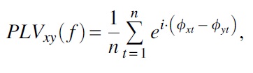
where, f = frequency of interest, n = number of time points (t) in the epoch, i = imaginary number, and ϕ_x and ϕ_x = phase angles from two signals x and y with the frequency of interest.

Spurious results outside selected frequency ranges were ignored (BESA Connectivity, 2020). BESA Connectivity outputs were converted to a BESA Statistics-compatible format in MATLAB v2020a using BESA-generated scripts. Three-dimensional head plots depicting changes in connectivity between brain regions were generated using BrainNet Viewer (Xia et al., 2013).

Statistical analyses

WM behavior was analyzed using custom MATLAB (v2020a) scripts. Performance is reported as percent correct out of total possible trials. Reaction time is reported as mean reaction time for responses across all trials. The kurtosis and skewness of performance and reaction time was evaluated in SPSS v24.0. Nonparametric statistics using the related samples Wilcoxon Signed-Rank Test were computed after reviewing skewness and kurtosis of each dependent variable. Since behavioral distributions indicated moderate skewness and kurtosis, a nonparametric paired-samples test was used for performance comparisons.

Three subjects who produced many no response trials on either the low- or high-load condition were initially included in the behavioral analysis and subsequent EEG comparisons. These subjects were excluded from the correct trials only analysis (see Supplementary Data S1), and the behavioral analysis was repeated excluding these subjects. Excluding these three subjects did not change the behavioral findings. The results reported below also exclude them. Regression and point plots of behavioral performance and mean delay activity were run in Python v3.6 using Seaborn v0.11.1 and can be found in Supplementary Data S1.

Delay activity analyses were carried out in BESA Statistics v 2.0, which handles multiple comparisons by permutation tests producing cluster and associated probability values (Maris and Oostenveld, 2007). Paired t-tests were used for delay activity comparisons across conditions, followed by correlations with behavioral measures. The cluster value is a sum of t-values for a t-test and a sum of r-values for correlation across a group of adjacent bins. A bin consists of sensors that are <4 cm distance, latency of 100 msec, and frequency bins of 0.5 Hz. A null distribution is created by sampling randomly from clusters across subjects and across time–frequency bins.

Significant clusters are summed t- or r-values within a specific time–frequency bin that exceeds a specific threshold, which are then compared with the random null distribution created from 1000 permutations (Bullmore et al., 1999; Ernst, 2004; Freedman and Lane, 1983; Maris and Oostenveld, 2007; O'Gorman, 2012).

Clusters were considered significant at p ≤ 0.05. Significant clusters are indicated with a mask colored either blue or orange. Orange represents low greater than high load, and blue represents high greater than low load for the TFA and TSA (event-related synchronization) comparisons. For connectivity, significant clusters are indicated with red representing greater phase locking for low compared with high load, and blue representing greater phase locking for high compared with low load.

Results

Behavioral

Low- and high-load WM performance was significantly different (Fig. 2, low-load 94.74%, SD 6.37, high-load 86.21%, SD 10.24, related samples Wilcoxon signed-rank test, p = 0.001). Low-load WM trial reaction times were faster than for high-load (low-load 878.62 msec, SD 139.76, high-load 955.71 msec, SD 122.02, related samples Wilcoxon signed-rank test, p = 0.002).

FIG. 2.

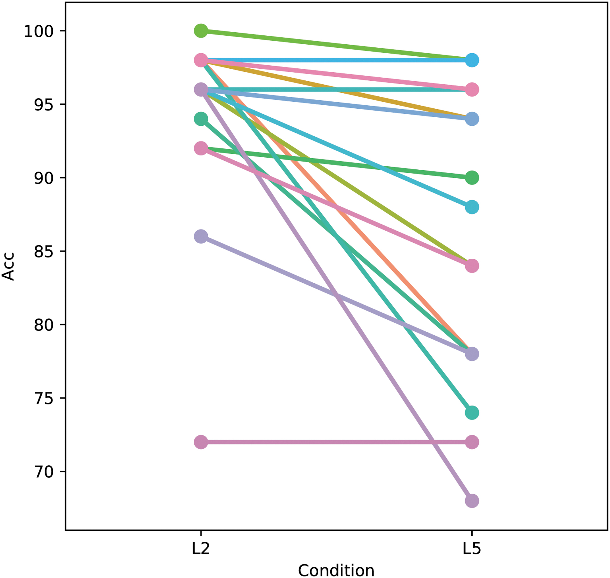
Better performance on the scene WM task for the low- than the high-load condition. Point plot of performance on the low- (L2) and high-load (L5) WM tasks. Each line in the figure represents a subject. Performance was significantly better on the low- compared with the high-load condition (94.6% correct vs. 86.2%, Wilcoxon Signed-Rank Test p = 0.001). Each color represents an individual subject. Accuracy (Acc) was defined as percentage of trials correct out of total possible trials. Three subjects with a large number of no response trials were excluded.

Absolute amplitude

Sensor-level comparison of low- and high-load delay period absolute amplitude revealed five significantly different clusters of delay activity (Table 1). Four of the five clusters revealed greater amplitude for the low- versus high-load condition throughout the entire delay period (0–6000 msec) spanning all frequencies. The clusters were mainly in the alpha and beta ranges, with greater amplitude for the low- compared with high-load condition (Fig. 3a–c). The remaining cluster showed a greater amplitude for the high-load condition in the first half of the delay period (0–2600 msec). This cluster encompassed right centro-frontal channels (F4′_avr, C4′_avr, FC6′_avr, and CP6′_avr) and included the upper beta and gamma range (29–37 Hz). This analysis used all delay period trials, regardless of correct or incorrect probe response.

FIG. 3.

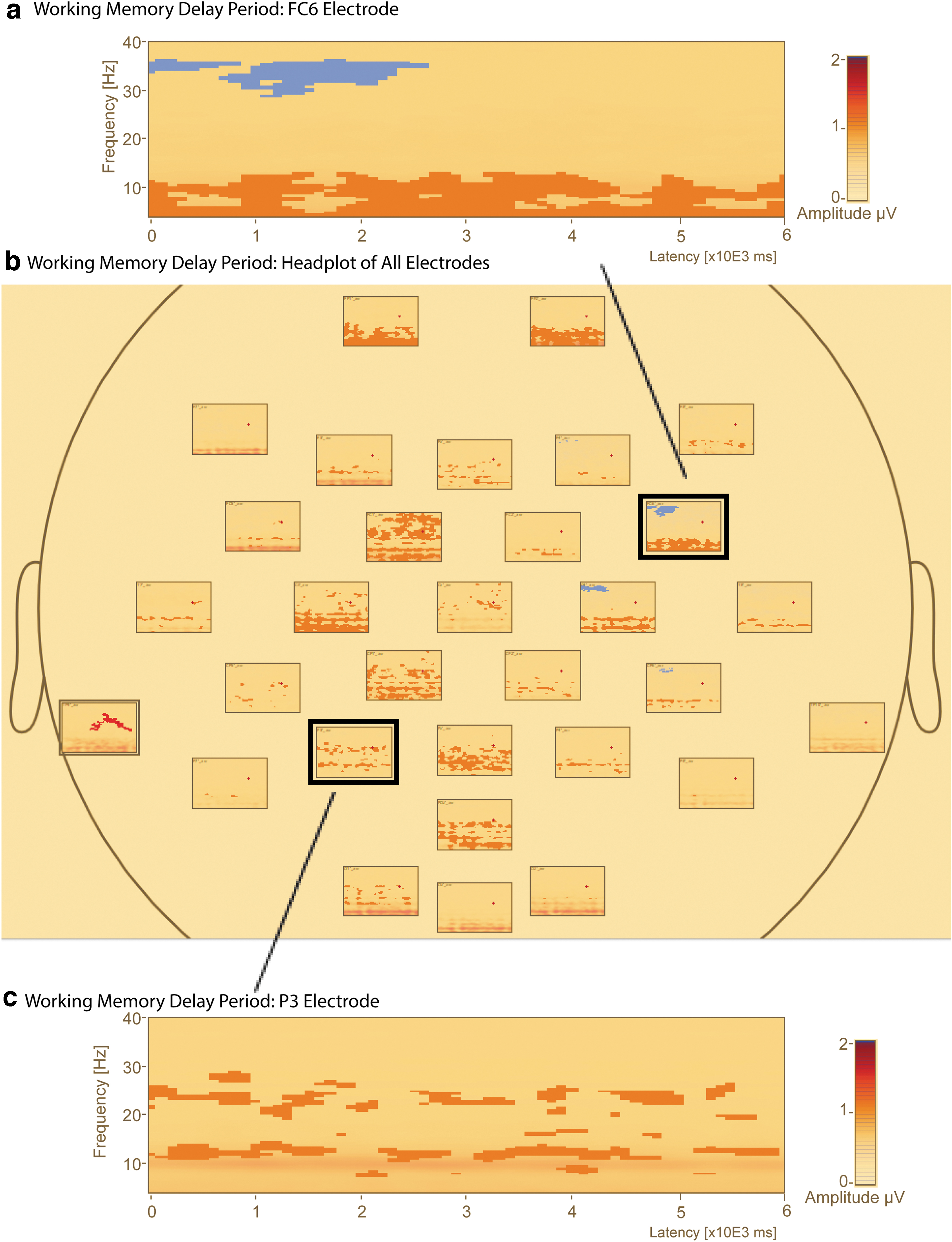
Comparison of absolute amplitude delay period activity in low- and high-load conditions reveals greater alpha and beta band amplitude across the delay period. Select absolute amplitude plots in the left frontal and right parietal regions of the delay period revealed five clusters of significant differences in activity (p < 0.05). Orange clusters represent low-load delay activity greater than high load, while blue clusters represent high-load delay activity greater than low load. The y-axis shows frequency (Hz); x-axis shows the time in sec. (a) Time–frequency absolute amplitude plot for the FC6 electrode. The plot shows the low-load condition absolute amplitude with the significant clusters overlaid as a mask. (b) Head plot of the overall pattern of absolute amplitude difference during the delay period for all sensors. (c) Time–frequency absolute amplitude plot for the P3 electrode. The plot shows the low-load condition Absolute Amplitude with the significant clusters overlaid as a mask. The selected FC6 (a) and P3 (c) electrodes are highlighted by a dark box on the head plot (b).

Table 1.

Significant Clusters of Absolute Amplitude Difference Between the Low- (L2) and High-Load (L5) Conditions During the Delay Period (Time: 0 to 6000 msec) for All Sensors

Cluster ID	p	Cluster value	Mean for L2 Abs Amp	Mean for L5 Abs Amp	Start time	End time	Start frequency	End frequency	Electrodes in cluster
Cluster 1	0.001	25837.9	0.958192	0.761117	0	6000	4	40	F3′_avr, F4′_avr, C3′_avr, C4′_avr, P3′_avr, P4′_avr, O1′_avr, O2′_avr, F8′_avr, T7′_avr, T8′_avr, P7′_avr, P8′_avr, Fz′_avr, Cz′_avr, Pz′_avr, FC1′_avr, FC2′_avr, CP1′_avr, CP2′_avr, FC5′_avr, FC6′_avr, CP5′_avr, CP6′_avr, POz′_avr
Cluster 2	0.016	3093.72	1.17774	0.842218	0	6000	4	20.5	FP1′_avr
Cluster 3	0.016	3046.2	1.23239	0.889094	0	6000	4	18.5	FP2′_avr
Cluster 4	0.044	−905.505	0.439429	0.547827	0	2600	29	37	F4′_avr, C4′_avr, FC6′_avr, CP6′_avr
Cluster 5	0.047	544.782	0.717711	0.630565	2300	5600	19	31.5	TP9′_avr

To investigate whether activity during incorrect responses may have influenced this difference, a separate analysis examined the relationship between activity in selected significant clusters with performance (Supplementary Fig. S3a–d), but included only delay periods for trials with correct responses.

Temporal spectral amplitude

A sensor-level comparison of low- and high-load delay period TSA revealed a transient pattern of delay activity that was most pronounced in the right parietal region (Fig. 4a, b, P8), similar to previous studies from our laboratory (Ellmore et al., 2017; Plaska et al., 2021). There was one cluster of significantly different TSA delay activity found early in the delay period (time = 300–2500 msec). TSA at low load exhibited greater event-related desynchrony (ERD) than high-load (Fig. 4b, c; cluster value = −1337.84, p = 0.013) in the upper beta and gamma range (frequency = 29.5–40 Hz).

FIG. 4.

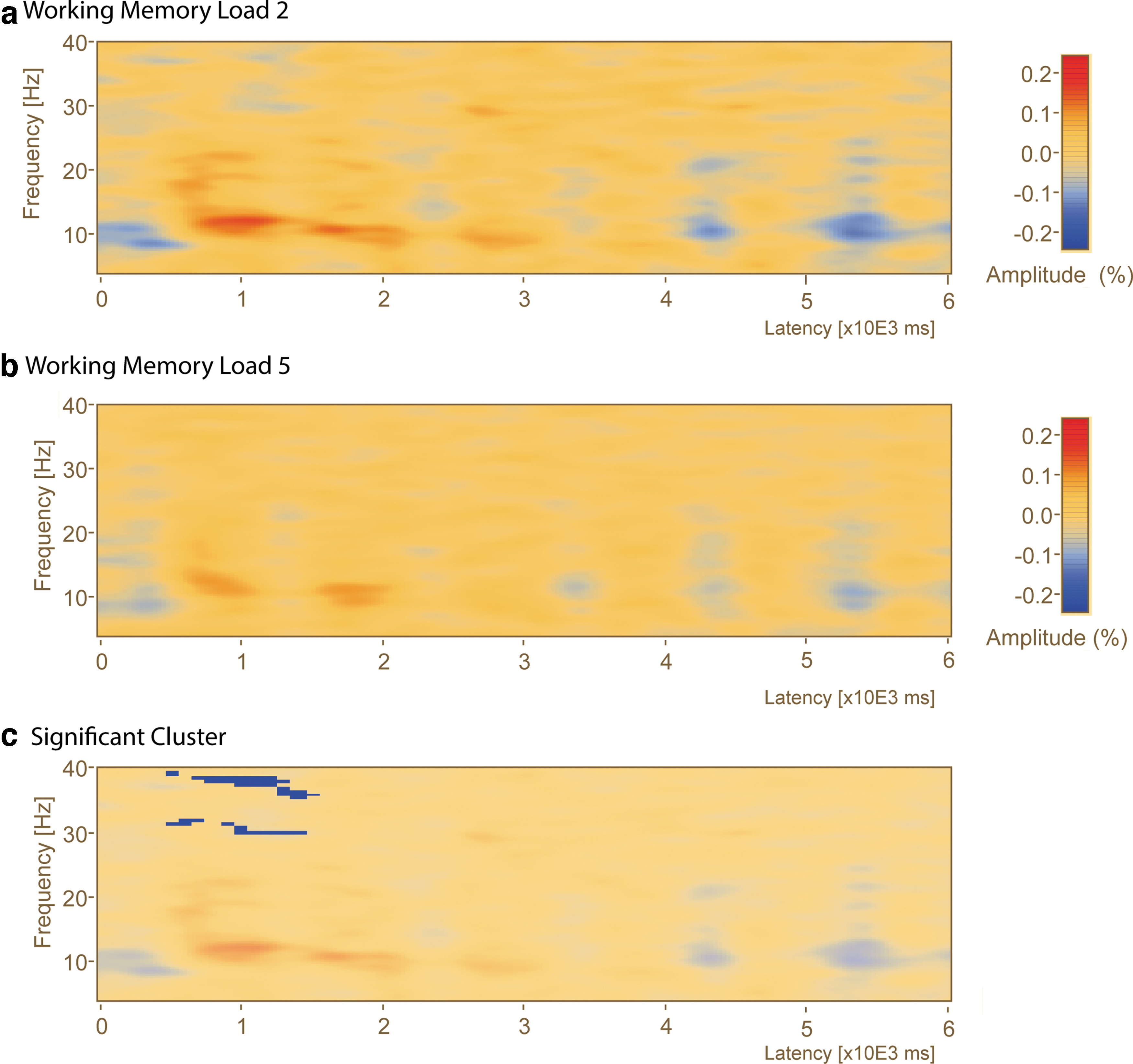
Comparison of delay period time–frequency between low- and high-load conditions reveals early gamma band ERD. A whole window time–frequency analysis plot for the P8 electrode selected based on results from previous research in our laboratory highlighting the importance of the right parieto-occipital region (Ellmore et al., 2017) for this task. (a) Time–frequency analysis for the P8 electrode in the low-load condition. (b) Time–frequency analysis for the P8 electrode in the high-load condition. (c) The plot shows the time–frequency analysis plot from the low-load condition with the significant load difference cluster overlaid as a mask. The blue cluster represents reduced ERD for the high-load condition. A review of the overall pattern of delay activity between the low- and high-loads reveals a similar transient pattern of delay activity for the parieto-occipital censors with an early period of increased synchronous activity in the upper alpha and beta bands (500–3000 msec) followed by a period of desynchronous activity in the same frequency bands (4000–6000 msec). ERD, event-related desynchrony.

Temporal spectral amplitude source analysis

A brain region source-level comparison of low- and high-load delay period TSA found two clusters of significantly different delay activity (Fig. 5). The left frontal region exhibited greater event-related synchronization in the low- compared with high-load condition during the first half of the delay period (Cluster 1: cluster value = 176.60, p = 0.003, frequency = 4–8.5 Hz, event-related synchrony greater during low load, time = 2700–3300 msec at source FL_BR). The left temporoparietal region exhibited greater event-related desynchronization for the low compared with high-load condition (Cluster 2: cluster value = −134.03, p = 0.036, frequency = 22.5–27 Hz, ERD greater for low load, time = 1800–2600 msec at source TPL_BR) in the middle of the delay period.

FIG. 5.

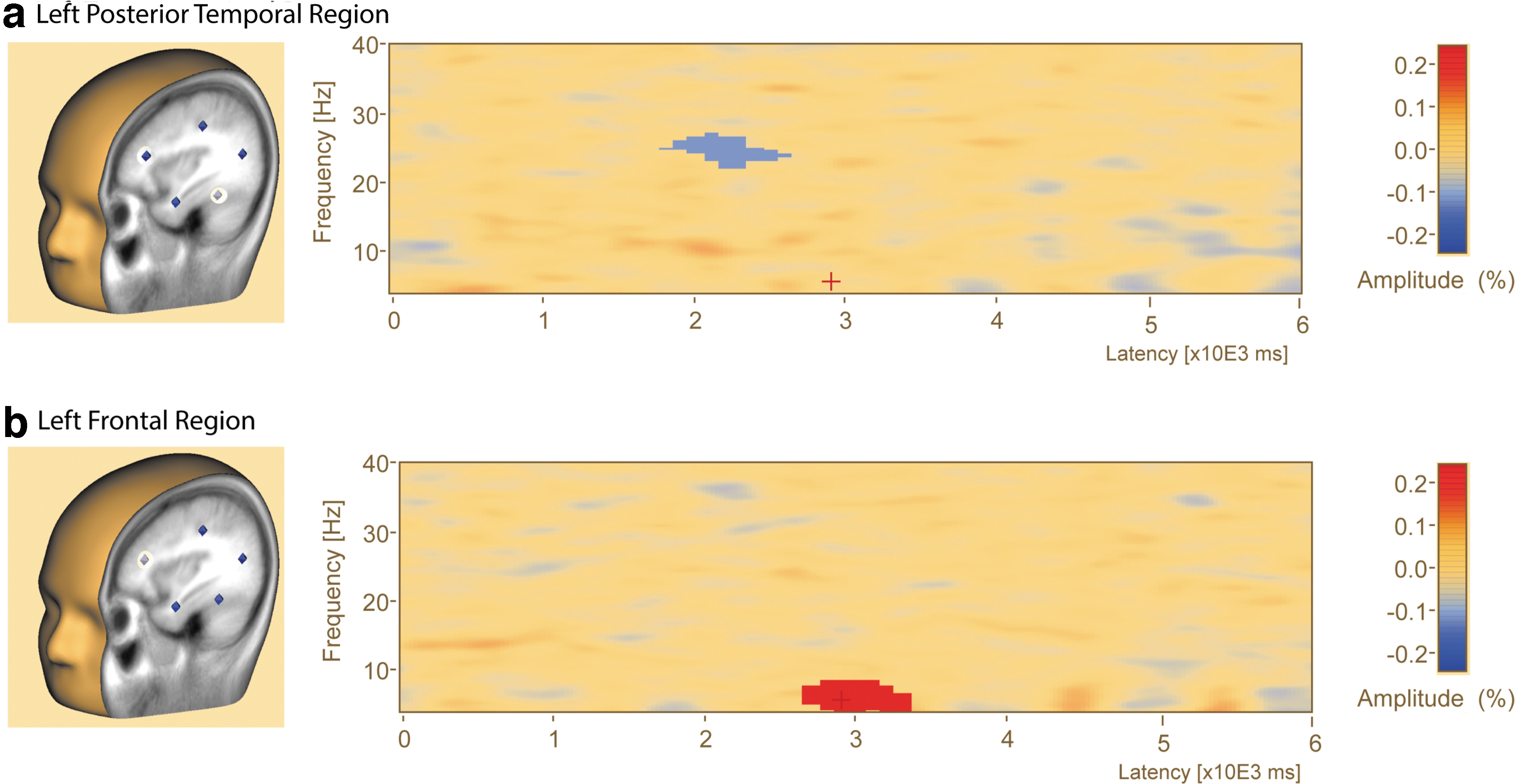
Delay period activity source analysis reveals changes in left posterior temporal and left frontal regions during maintenance. Time–frequency analysis plots during the delay period during the brain regions source analysis. (a) 3D view of Brain Regions’ Montage superimposed on an MRI structural scan with the left posterior temporal region highlighted in yellow (left). Time–frequency analysis for the left posterior temporal region during the delay period (right). The blue cluster represents greater ERD in the upper beta range for the low-load condition. (b) 3D view of Brain Regions’ Montage superimposed on a template MRI structural scan with the left frontal region highlighted in yellow (left). Time–frequency analysis for the left frontal during the delay period (right). The red cluster represents greater ERS in the theta and alpha range for the low-load condition. 3D, three-dimensional; ERS, event-related synchrony; MRI, magnetic resonance imaging.

PLV source analysis

PLV for both the low- and high-load conditions appeared sustained throughout the entire delay period (Fig. 6). A paired-samples t-test with corrections for multiple comparisons revealed significantly different clusters between low and high load (Table 2). There were three clusters of significantly different PLV, including a cluster between left frontal and right posterior temporal sources (Fig. 7a, cluster value = 1120.94, p = 0.024, frequency range 4–9.5 Hz, time range 0–6000 msec, sources FL_BR–TPR_BR).

FIG. 6.

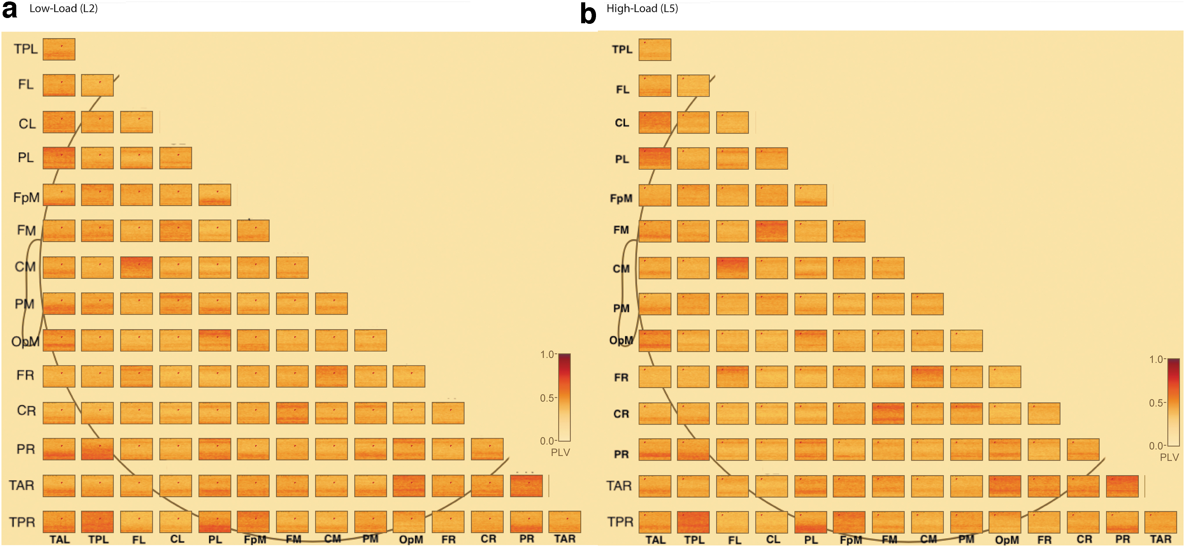
PLV connectivity matrices for the low- and high-load conditions. Each subplot represents a matrix of connections among 15 brain regions (see Methods section) within a condition, averaged across trials and subjects. For each matrix, the major X and Y axis contain labels for the brain regions. Each box inside the matrix represents 1 connection (e.g., top left box to connection between left posterior temporal to left anterior temporal). For each box, the plot shows the PLV for that connection and displays PLV on a scale from 0 to 1, with 0 (yellow color) indicating no connectivity and 1 (deep red) indicating highest level of connectivity. For each box, the Y axis is frequency from 4 to 40 Hz and the X axis represents the full delay period (0–6000 msec). 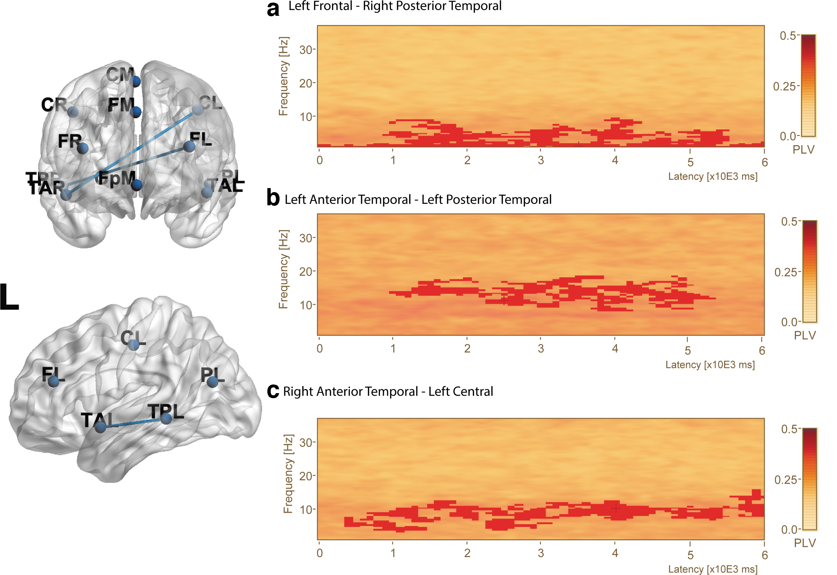(a) Connectivity matrix for the low-load condition (L2). (b) Connectivity matrix for the high-load condition (L5). Both the low- and high-load conditions appear to have sustained levels of PLV throughout the entire delay period (see PLV source analysis section). PLV, phase-locking values.

FIG. 7.

PLV during the delay period reveal three different connections with higher connectivity during the low-load condition. The plots show PLV during the delay period in a brain regions’ connectivity analysis. A 3D transparent brain frontal (left-top) and left lateral view (left-bottom) displaying the significantly different PLV connections highlighted with a blue connection line. Letters on the 3D brain letters refer to locations: L = left hemisphere, R = right hemisphere, A = anterior, P = posterior, T = temporal lobe, P = parietal lobe, and F = frontal lobe. (a) Connectivity plot for the connection between left frontal and right posterior temporal regions with mask of the significant cluster indicating that the low-load condition had greater connectivity between these two regions than the high-load condition (red mask, p = 0.024). (b) Connectivity plot of the connection between the left anterior temporal and left posterior temporal regions indicating that the low-load condition had greater connectivity than the high-load condition (red mask, p = 0.027). (c) Connectivity plot of the connection between right anterior temporal and the left central regions indicating that the low-load condition had greater connectivity between these two regions than the high-load condition (red mask, p = 0.022).

Table 2.

Significant Clusters of Phase-Locking Value Between 15 Brain Regions During the Delay Period (Time: 0–6000 msec)

Cluster ID	p	Cluster value	Mean for L2 PLV	Mean for L5 PLV	Start time	End time	Start frequency	End frequency	Phase-locking regions
Cluster 1	0.022	1132.9	0.3342	0.223609	400	6000	4^*	16	CL_BR to TAR_BR
Cluster 1	0.022	1132.9	0.3342	0.223609	400	6000	4^*	16	TAR_BR to CL_BR
Cluster 2	0.024	1120.94	0.343857	0.217204	0	6000	4^*	9.5	FL_BR to TPR_BR
Cluster 2	0.024	1120.94	0.343857	0.217204	0	6000	4^*	9.5	TPR_BR to FL_BR
Cluster 3	0.027	975.112	0.346558	0.247562	1000	5300	8.5	18.5	TAL_BR to TPL_BR
Cluster 3	0.027	975.112	0.346558	0.247562	1000	5300	8.5	18.5	TPL_BR to TAL_BR

Erroneous results outside the selected frequency range were ignored.

Each PLV connection between the low- (L2) and high-load (L5) conditions has two significant clusters associated with it to represent the opposite connection (e.g., PL–FL and FL–PL). The PLV results do not provide information about the directionality. The start frequency for all comparisons was 4 Hz, but can erroneously report frequencies lower (i.e., lower than 4 Hz), so start indicates numbers that were adjusted due to erroneous values (see Methods section).

PLV, phase-locking value.

There was also greater PLV between left frontal and right posterior temporal regions in the theta and alpha ranges throughout the entire delay period. There was a significant difference in PLV between left anterior temporal and left posterior temporal (Fig. 7b, cluster value = 975.11, p = 0.027, frequency range 8.5–18 Hz, time range 1000–5300 msec, sources TAL_BR–TPL_BR).

There was significantly greater PLV between left anterior temporal and left posterior temporal regions in the alpha and lower beta ranges throughout the entire delay period. There was a significant difference in PLV between left central and right anterior temporal regions (Fig. 7c, cluster value = 1132.9, p = 0.022, frequency range 4–16 Hz, time range 400–6000 msec, sources CL_BR–TAR_BR). There was greater PLV between the left central and right anterior temporal regions in the theta, alpha, and lower beta ranges starting after about 400 msec and continuing until the end of the delay period. An exploratory analysis was conducted to examine if incorrect responses influenced the results (Supplementary Figs. S4–S6).

Correlations with behavior

Correlations between performance and delay activity showed no significant correlations between TSA delay activity and performance for either condition (low-load p-value = 0.09; high-load p-value = 0.32). There were also no significant correlations between the PLV and performance for either condition (low-load p-value = 0.80; high-load p-value = 0.63).

Discussion

We tested the hypothesis that introducing perceptually similar visual information during the delay period would engage attention and distract from maintenance in a load-dependent manner.

We found results consistent with this hypothesis with performance being better in a low-load WM condition as well on an immediate recognition task for stimuli from the low-load condition. This finding is consistent with the literature on WM load; however, load manipulation studies typically use simple stimuli that are easy to name and do not elicit meaningful connections between the stimulus features and stored knowledge (Asp et al., 2021; Plaska et al., 2021). Consequently, the attention-consuming process of associating meaning to the picture may have used up the available attentional resources and the interfering stimuli may have had no impact on performance. We argue that the interfering stimuli did interfere with maintenance and negatively impact performance as evidenced by the reduced delay activity for the high load.

We predicted that there at the low load, this interference was predicted to have less of an impact on delay activity and connectivity. Thus, performance would be better than the high-load condition, delay activity would be persistent, and connectivity in frontal and parietal regions would be greater for the low-load condition.

We found patterns in our results that are consistent with these predictions. There was greater above-baseline amplitude in alpha and lower beta bands for the low-load condition across most sensors, although overall TSA was more transient in nature. Greater amplitude in the alpha and lower beta range in the low-load condition could reflect greater disruption of attention for the high-load condition by the interfering stimuli (Bonnefond and Jensen, 2012). It may also reflect that during low-load WM maintenance there were more resources available to process the interfering stimuli (Yoon et al., 2006) and the available resources could have been used to deal with the interference.

While greater activation of the parietal region during the high-load condition would be consistent with traditional accounts of WM processing scaling positively with the amount of information being maintained, lower activity may instead reflect a different neural mechanism such as activity-silent storage (Stokes et al., 2020) to deal with interference during the delay. Alternatively, the greater perceptual load during the high-load condition may have resulted in a reduced distractor effect on delay activity (Lavie et al., 2004), while greater amplitude in the low-load condition could reflect maintenance of both target and interfering stimuli.

Differences in connectivity between the low- and high-load conditions were found with greater connectivity during the delay period between the left central and right anterior temporal regions in an analysis of all trials and in a separate analysis of only trials with correct responses. The central region is located superiorly near the junction of the frontal and parietal lobes, potentially overlapping with the anterior portion of the posterior parietal cortex (PPC) (Whitlock, 2017).

The PPC is involved in attentional processes (Hutchinson et al., 2009) with more dorsal regions associated with allocating and control of attention. Increased connectivity among occipital, temporal, and parietal regions, including PPC, has been reported with increased WM load. Specifically, increases in lower frequency bands, such as alpha and lower beta, are attributed to the deployment of attentional resources (Palva et al., 2010, 2011).

Increased connectivity between left central and right anterior temporal regions within these lower frequency bands may reflect control of attention for the maintained stimuli, which was likely easier at a low load of two stimuli compared with five stimuli, and which is important for preventing the degradation of the WM representation (Lorenc et al., 2021). Significant connectivity in the simultaneously collected fMRI data was also found between these regions (see Supplementary Data S1), but with the opposite relation (high > low load) possibly due to the negative correlation between fMRI-blood oxygen level dependent signal and alpha/theta during WM tasks (Meltzer et al., 2007).

There was greater connectivity between left frontal and right posterior temporal regions, and between left anterior temporal and left posterior temporal regions. Left frontal regions are important for filtering interference and increased attentional selection (Gazzaley and Nobre, 2012; Jha et al., 2004). The right posterior temporal region could be consistent with storage of the encoded stimuli as Park and colleagues (2011) proposed that superior temporal gyrus represents a store for complex visual stimuli.

Filtering associated with complex stimuli used here would be essential for correct responses. Consistent with this idea, significant differences in this network emerged only when all trials were included in the analysis and were no longer present when examining only correct trials. If this network supports the filtering of interfering stimuli during the maintenance of complex stimuli, then the observation that there was no significant difference between the low- and high-load delay periods (when examining correct only trials) suggests that filtering was critical for successful performance.

There was also an increase in connectivity between left anterior temporal and left temporoparietal regions. The left anterior temporal region is important for language, short-term memory, and semantic associations (Boucher et al., 2015; Helmstaedter et al., 1996; Hermann et al., 1992). The left posterior temporal region has been implicated in word processing and comprehension (Binder et al., 1997). Phase locking between these regions was restricted to the alpha and lower beta regions, which suggests this connection represents feedback from the anterior temporal to the posterior region throughout the latter half of the delay period (about 1000–5000 msec). This may be related to the stimulus being recoded into a label using an association of stored semantic knowledge followed by rehearsal.

Even without explicit instructions, participants could adopt a strategy involving verbal recoding and rehearsal, particularly with stimuli that contain high semantic content (Brown et al., 2006) like the scenes used here.

Increased connectivity was observed during the low-load condition, consistent with behavioral observations and subject self-reports that it is easier to rehearse two stimuli recoded with semantic associations than it is to rehearse five. In the high-load condition, participants may have had to rely on an alternate less-efficient maintenance strategy (Chen and Cowan, 2009) like gist-based attentional refreshing, which may explain worse performance at high loads. Additionally, reduced connectivity in the high-load condition may imply that a load of five taxed participants’ WM capacity, especially considering the stimuli, were complex scenes (Zhang et al., 2016).

Conclusions

Interference during the visual WM delay period impacted maintenance for complex stimuli in a load-dependent manner. Successful maintenance at low load, as evidenced by better performance and greater delay activity, could be the result of filtering interfering stimuli, the ability to focus attention on maintenance, and the application of verbal maintenance strategies.

At the neural level, greater reductions in amplitude were observed in the alpha and beta ranges at high load, which may reflect a distractor effect or reliance on activity-silent mechanisms. The latter is less likely as only the low-load condition was supported by increased left frontal–right posterior temporal, left anterior temporal–posterior temporal, and right anterior temporal–left central connectivity suggesting that both intra- and inter-hemispheric interactions may support WM maintenance of complex visual stimuli.

Footnotes

Acknowledgments

The authors thank A. Duke Shereen, PhD and Kenneth Ng for their help with task set-up and with data collection. They want to thank Farzana Antara, Gabriela Silva, and Albert Perdomo for help with EEG data processing. They also want to thank Michael Epstein, PhD for his constructive feedback on the article.

Authors’ Contributions

T.M.E. conceived the experiment, obtained funding, and developed the task. C.R.P., J.O., and B.A.G. carried out EEG preparation, data collection, and carried out all data processing. C.R.P. carried out all data analysis and wrote the article. J.O. and B.A.G. reviewed and provided feedback on the article. T.M.E. aided in interpreting the results and writing the article as well as supervised all aspects of the experiment.

Availability of Data

Deidentified data will be made available upon reasonable request to the corresponding author.

Author Disclosure Statement

No competing financial interests exist.

Funding Information

This experiment was funded by a CUNY ASRC Seed Grant (Round 4) and NIH R56MH116007.

Supplementary Material

Supplementary Data S1

References

Allen

, Josephs

, Turner

. 2000. A method for removing imaging artifact from continuous EEG recorded during functional MRI. Neuroimage, 12:230–239.

Alvarez

, Cavanagh

. 2004. The capacity of visual short-term memory is set both by visual information load and by number of objects. Psychol Sci, 15:106–111.

Asp

, Störmer

, Brady

. 2021. Greater visual working memory capacity for visually matched stimuli when they are perceived as meaningful. J Cogn Neurosci, 33:902–918.

Awh

, Barton

, Vogel

. 2007. Visual working memory represents a fixed number of items regardless of complexity. Psychol Sci, 18:622–628.

Babiloni

, Babiloni

, Carducci

, et al. 2004. Functional frontoparietal connectivity during short-term memory as revealed by high-resolution EEG coherence analysis. Behav Neurosci, 118:687.

BESA Connectivity. 2020. BESA Connectivity Manual 1.0. Germany: ESA^® GmbH. ftp://h1772544.stratoserver.net/public/Connectivity/BESA%20Connectivity%201.0%20-%20User%20Manual.pdf Last accessed Mar. 10, 2022 .

BESA Research

WIKI

. 2020. Pipeline for simultaneous EEG fMRI. http://wiki.besa.de/index.php?title=Pipeline_for_simultaneous_EEG-fMRI_recording Last accessed Mar. 10, 2022 .

Beukers

, Buschman

, Cohen

, et al. 2021. Is activity silent working memory simply episodic memory?. Trends Cogn Sci, 25:284–293.

Binder

, Frost

, Hammeke

, et al. 1997. Human brain language areas identified by functional magnetic resonance imaging. J Neurosci, 17:353–362.

10.

Bollinger

, Rubens

, Zanto

, et al. 2010. Expectation-driven changes in cortical functional connectivity influence working memory and long-term memory performance. J Neurosci, 30:14399–14410.

11.

Bonnefond

, Jensen

. 2012. Alpha oscillations serve to protect working memory maintenance against anticipated distracters. Curr Biol, 22:1969–1974.

12.

Boucher

, Dagenais

, Bouthillier

, et al. 2015. Different effects of anterior temporal lobectomy and selective amygdalohippocampectomy on verbal memory performance of patients with epilepsy. Epilepsy Behav, 52:230–235.

13.

Brown

, Forbes

, McConnell

. 2006. Short article: limiting the use of verbal coding in the visual patterns test. Quart J Exp Psychol, 59:1169–1176.

14.

Bullmore

, Suckling

, Overmeyer

, et al. 1999. Global, voxel, and cluster tests, by theory and permutation, for a difference between two groups of structural MR images of the brain. IEEE Trans Med Imaging, 18:32–42.

15.

Chen

, Cowan

. 2009. How verbal memory loads consume attention. Mem Cogn, 37:829–836.

16.

Constantinidis

, Funahashi

, Lee

, et al. 2018. Persistent spiking activity underlies working memory. J Neurosci, 38:7020–7028.

17.

Ellmore

, Ng

, Reichert

. 2017. Early and late components of EEG delay activity correlate differently with scene working memory performance. PLoS One, 12:e0186072.

18.

Ernst

. 2004. Permutation methods: a basis for exact inference. Stat Sci, 19:676–685.

19.

Feredoes

, Heinen

, Weiskopf

, et al. 2011. Causal evidence for frontal involvement in memory target maintenance by posterior brain areas during distracter interference of visual working memory. Proc Natl Acad Sci, 108:17510–17515.

20.

Freedman

, Lane

. 1983. A nonstochastic interpretation of reported significance levels. J Bus Econ Stat, 1:292–298.

21.

Gazzaley

, Nobre

. 2012. Top-down modulation: bridging selective attention and working memory. Trends Cogn Sci, 16:129–135.

22.

Gazzaley

, Rissman

, D'esposito

. 2004. Functional connectivity during working memory maintenance. Cogn Affect Behav Neurosci, 4:580–599.

23.

Goldman-Rakic

. 1995. Cellular basis of working memory. Neuron, 14:477–485.

24.

Hampson

, Driesen

, Skudlarski

, et al. 2006. Brain connectivity related to working memory performance. J Neurosci, 26:13338–13343.

25.

Heinz

, Johnson

. 2017. Load-dependent increases in delay-period alpha-band power track the gating of task-irrelevant inputs to working memory. Front Hum Neurosci, 11:250.

26.

Helmstaedter

, Elger

, Hufnagel

, et al. 1996. Different effects of left anterior temporal lobectomy, selective amygdalohippocampectomy, and temporal cortical lesionectomy on verbal learning, memory, and recognition. J Epilepsy, 9:39–45.

27.

Hermann

, Wyler

, Bush

, et al. 1992. Differential effects of left and right anterior temporal lobectomy on verbal learning and memory performance. Epilepsia, 33:289–297.

28.

Hoechstetter

, Bornfleth

, Weckesser

, et al. 2004. BESA source coherence: a new method to study cortical oscillatory coupling. Brain Topogr, 16:233–238.

29.

Hutchinson

, Uncapher

, Wagner

. 2009. Posterior parietal cortex and episodic retrieval: convergent and divergent effects of attention and memory. Learn Mem, 16:343–356.

30.

Ille

, Berg

, Scherg

. 2002. Artifact correction of the ongoing EEG using spatial filters based on artifact and brain signal topographies. J Clin Neurophysiol, 19:113–124.

31.

Jensen

, Gelfand

, Kounios

, et al. 2002. Oscillations in the alpha band (9–12 Hz) increase with memory load during retention in a short-term memory task. Cereb Cortex, 12:877–882.

32.

Jensen

, Mazaheri

. 2010. Shaping functional architecture by oscillatory alpha activity: gating by inhibition. Front Hum Neurosci, 4:186.

33.

Jensen

, Tesche

. 2002. Frontal theta activity in humans increases with memory load in a working memory task. Eur J Neurosci, 15:1395–1399.

34.

Jha

, Fabian

, Aguirre

. 2004. The role of prefrontal cortex in resolving distractor interference. Cogn Affect Behav Neurosci, 4:517–527.

35.

Kamiński

, Rutishauser

. 2020. Between persistently active and activity-silent frameworks: novel vistas on the cellular basis of working memory. Ann N Y Acad Sci, 1464:64.

36.

Lachaux

, Rodriguez

, Martinerie

, et al. 1999. Measuring phase synchrony in brain signals. Hum Brain Mapp, 8:194–208.

37.

Lavie

. 1995. Perceptual load as a necessary condition for selective attention. J Exp Psychol, 21:451.

38.

Lavie

, Hirst

, De Fockert

, et al. 2004. Load theory of selective attention and cognitive control. J Exp Psychol, 133:339.

39.

Lorenc

, Mallett

, Lewis-Peacock

. 2021. Distraction in visual working memory: resistance is not futile. Trends Cogn Sci, 25:228–239.

40.

Maris

, Oostenveld

. 2007. Nonparametric statistical testing of EEG-and MEG-data. J Neurosci Methods, 164:177–190.

41.

Meltzer

, Negishi

, Mayes

, et al. 2007. Individual differences in EEG theta and alpha dynamics during working memory correlate with fMRI responses across subjects. Clin Neurophysiol, 118:2419–2436.

42.

Mullinger

, Yan

, Bowtell

. 2011. Reducing the gradient artefact in simultaneous EEG-fMRI by adjusting the subject's axial position. Neuroimage, 54:1942–1950.

43.

O'Gorman

. 2012. Adaptive Tests of Significance Using Permutations of Residuals with R and SAS. Hoboken, NJ: John Wiley &. Sons.

44.

Palva

, Monto

, Kulashekhar

, et al. 2010. Neuronal synchrony reveals working memory networks and predicts individual memory capacity. Proc Natl Acad Sci, 107:7580–7585.

45.

Palva

, Kulashekhar

, Hämäläinen

, et al. 2011. Localization of cortical phase and amplitude dynamics during visual working memory encoding and retention. J Neurosci, 31:5013–5025.

46.

Papp

, Ktonas

. 1977. Critical evaluation of complex demodulation techniques for the quantification of bioelectrical activity. Biomed Sci Instrum, 13:135.

47.

Park

, Kang

, et al. 2011. Cross-frequency power correlations reveal the right superior temporal gyrus as a hub region during working memory maintenance. Brain Connect, 1:460–472.

48.

Pfurtscheller

. 2001. Functional brain imaging based on ERD/ERS. Vision Res, 41:1257–1260.

49.

Pfurtscheller

, Da Silva

. 1999. Event-related EEG/MEG synchronization and desynchronization: basic principles. Clin Neurophysiol, 110:1842–1857.

50.

Picton

, van Roon

, Armilio

, et al. 2000. The correction of ocular artifacts: a topographic perspective. Clin Neurophysiol, 111:53–65.

51.

Plaska

, Ng

, Ellmore

. 2021. Does rehearsal matter? Left anterior temporal alpha and theta band changes correlate with the beneficial effects of rehearsal on working memory. Neuropsychologia, 155:107825.

52.

Sarnthein

, Petsche

, Rappelsberger

, et al. 1998. Synchronization between prefrontal and posterior association cortex during human working memory. Proc Natl Acad Sci, 95:7092–7096.

53.

Scheeringa

, Petersson

, Oostenveld

, et al. 2009. Trial-by-trial coupling between EEG and BOLD identifies networks related to alpha and theta EEG power increases during working memory maintenance. Neuroimage, 44:1224–1238.

54.

Scherg

. 1992. Functional imaging and localization of electromagnetic brain activity. Brain Topogr, 5:103–111.

55.

Scherg

, Berg

, Nakasato

, et al. 2019. Taking the EEG back into the brain: the power of multiple discrete sources. Front Neurol, 10:855.

56.

Sreenivasan

, Curtis

, D'Esposito

. 2014. Revisiting the role of persistent neural activity during working memory. Trends Cogn Sci, 18:82–89.

57.

Sternberg

. 1966. High-speed scanning in human memory. Science, 153:652–654.

58.

Stokes

. 2015. ‘Activity-silent'working memory in prefrontal cortex: a dynamic coding framework. Trends Cogn Sci, 19:394–405.

59.

Stokes

, Muhle-Karbe

, Myers

. 2020. Theoretical distinction between functional states in working memory and their corresponding neural states. Vis Cogn, 28:420–432.

60.

Tuladhar

, Huurne

, Schoffelen

, et al. 2007. Parieto-occipital sources account for the increase in alpha activity with working memory load. Hum Brain Mapp, 28:785–792.

61.

Whitlock

. 2017. Posterior parietal cortex. Curr Biol, 27:R691–R695.

62.

Xia

, Wang

, He

. 2013. BrainNet Viewer: a network visualization tool for human brain connectomics. PLoS One, 8:e68910.

63.

Xiao

, Hays

, Ehinger

, et al. 2010. Sun database: large-scale scene recognition from abbey to zoo. 2010 IEEE Conference on Computer vision and pattern recognition (CVPR), San Francisco, CA:. IEEE.

64.

Yoon

, Curtis

, D'Esposito

. 2006. Differential effects of distraction during working memory on delay-period activity in the prefrontal cortex and the visual association cortex. Neuroimage, 29:1117–1126.

65.

Zhang

, Zhao

, Bai

, et al. 2016. Functional connectivity among multi-channel EEGs when working memory load reaches the capacity. Brain Res, 1631:101–112.

Supplementary Material

Please find the following supplemental material available below.

For Open Access articles published under a Creative Commons License, all supplemental material carries the same license as the article it is associated with.

For non-Open Access articles published, all supplemental material carries a non-exclusive license, and permission requests for re-use of supplemental material or any part of supplemental material shall be sent directly to the copyright owner as specified in the copyright notice associated with the article.

0.00 MB

2.96 MB

Interhemispheric Connectivity Supports Load-Dependent Working Memory Maintenance for Complex Visual Stimuli

Abstract

Introduction:

Methods:

Results:

Discussion:

Impact statement

Introduction

Methods

Participants

Memory tasks

EEG acquisition

EEG processing

Time–frequency analyses

Connectivity and phase-locking analyses

Statistical analyses

Results

Behavioral

Absolute amplitude

Temporal spectral amplitude

Temporal spectral amplitude source analysis

PLV source analysis

Correlations with behavior

Discussion

Conclusions

Footnotes

Acknowledgments

Authors’ Contributions

Availability of Data

Author Disclosure Statement

Funding Information

Supplementary Material

References

Supplementary Material