Revisiting Key Predistribution Using Transversal Designs for a Grid-Based Deployment Scheme

Abstract

We consider a grid-based deployment scheme in which keys are predistributed in sensor nodes following a transversal design. This scheme was first proposed by Ruj, Maitra, and Roy in [19]. In their scheme the RF region was considered to be the a square of appropriate dimension. In this article, we consider the RF region to be the Lee sphere of appropriate radius. This is a better approximation than the square RF region and all calculations of connectivity and resiliency is done with respect to this parameter.

1. Introduction

Sensor networks consist of resource constrained devices and deployed for both military and civilian purposes. To carry on communication in a secure manner, any two sensor nodes should communicate in an encrypted manner using a common secret key. Towards secure communication, it is important that any two sensor nodes should communicate in an encrypted manner using a common secret key. The designer may predistribute the keys in each sensor node or on-line key agreement strategies may be used. For on-line key agreement strategies, some kind of public key infrastructure is required. Public key techniques involve huge computational costs and are therefore not suitable for the resource constraint sensor nodes. Hence keys are preloaded in the sensors before deployment. Several key predistribution techniques have been discussed in literature. [1–4, 14–17].

To increase resiliency, deployment knowledge may be used. Deployment knowledge has been used in [1, 6, 7, 12, 15, 19, 21, 28]. In [19] Ruj, Maitra, and Roy proposed a grid-based deployment scheme in which keys are predistributed in the sensor nodes using combinatorial designs called transversal designs. As mentioned in [19], grid-based designs have several applications for both military and civilian purposes. They are used in intrusion detection as mentioned in [24] and [18]. Other applications of such a deployment pattern can be used to monitor temperature and pressure in a factory, monitor vehicles in a parking lot, monitor goods in a warehouse, monitor trees in a plantation. To protect commercial confidentiality, sensors may be placed in square grids. In this paper, we consider the grid-based deployment scheme where key predistribution is done according to the Transversal Design TD (k, r). We consider the Lee sphere while calculating the connectivity ratio and resiliency. We study the connectivity and resiliency of the network taking the Lee distance into account. The importance of such analysis of Lee distance lies in the fact that we can change the Lee distance according to power requirements.

Given any kind of deployment, the key predistribution techniques may be randomized, deterministic, or hybrid. Key predistribution in sensor networks was first discussed in by Eschenauer and Gligor in [9]. Other key predistribution schemes were discussed in [5, 8, 13–15, 23]. For application of combinatorial designs in key predistribution, one may refer to [2, 4, 16, 17, 20]. In particular, in [16] Lee and Stinson transversal designs for key predistribution has been presented that has been extended later in [4] by Chakrabarti, Maitra, and Roy.

We consider r² blocks (identify them as sensor nodes) of the TD which are placed on a deployment grid of dimension r × r. The connectivity of the network is then analyzed taking into account the Lee distance. The block indexed by (i, j) is placed in the (i, j) th location of the grid. We give a comparison of our scheme with that given by Ruj, Maitra, and Roy in [19]. We show how the connectivity ratio changes with the change of the Lee distance and number of keys in each node. The main idea where our proposal differs from the scheme given by Lee and Stinson [16] in that in their scheme sensor nodes are scattered randomly on an unknown geometry unlike our model where we consider a known grid based deployment.

The rest of this article is organized in the following way. In Section 2, we define basic concepts. In Section 3, we calculate the connectivity ratio (the fraction of nodes that a given node can communicate with within the Lee distance). For interior nodes we calculate the exact number of nodes with which it can communicate, for any given Lee distance. In Section 4, we study the resiliency of the network. We give two parameters for resiliency and find a tight theoretical bound for the first parameter and present experimental results for the second. We conclude in Section 5 with some open problems.

2. Preliminaries

A transversal design [26, Section 6.3] TD (k, λ; r), with k groups of size r and index λ, is a triple (X, G, A) where

X is a set of kr elements (varieties),

G = {G₁, G₂, …, G_k} is a family of k sets (each of size r) which form a partition of X,

A is a family of k-sets (or blocks) of varieties such that each k-set in A intersects each group G_i in precisely one variety, and any pair of varieties which belong to different groups occur together in precisely λ blocks in A.

We denote a transversal design with λ = 1 as TD(k, r). It can be shown that if there exists a TD(k, r), then there exists a (v, b, r, k) design with v = kr, b = r².

Let us now explain X, A in a transversal design TD(k, r).

X = {(x, y): 0 ≤ x < k, 0 ≤ y < r},

For all i, G_i = {(i, y): 0 ≤ y < r},

A = {A_i,j: 0 ≤ i < r & 0 ≤ j < r}.

We define a block A_i,j by

$$A_{i,j}=\{(x,xi+jmodr):0\le x<k\}$$

(1)

We consider an r × r grid such that there are r² points of intersection. For our purpose, we take a prime power r. We map the r² blocks to the r² sensor nodes and place block A_{i, j} at the location (i, j) of the grid as shown in Fig. 1a. We represent the node at (i, j) by n_{i, j}. The varieties are mapped on to the secret keys in the sensor nodes. Thus we establish a correspondence between TD(k, r) and the placement of sensor nodes on a r × r square grid. Note that any two blocks have either no key or one key in common and the algorithm to check whether the two nodes actually share a common secret key is efficient (see [16] for more details).

Figure 1.

A 7 × 7 grid with k = 3, ρ = 2. The physical neighbors of the node at (3, 3) occur along the dark lines and the key sharing neighbors are marked by crosses.

The sensor nodes can carry on effective communication only inside a particular range called the Radio Frequency (RF) range. The RF range with respect to a particular point is actually a circular region with center as that point and some radius around that. The Manhattan distance between two points is the sum of the horizontal and vertical distance between the points.

Consider a square grid (as shown in Fig. 1a). A Lee Sphere [1] of radius ρ centered at a given point P consists of the set of points that lie at a Manhattan distance of at most ρ from P. ρ is called the Lee distance. The triangle inequality implies that the Manhattan distance between two nodes is greater than the Euclidean distance. This implies that all the nodes within the Lee sphere of radius ρ centered at a point P are also contained in the RF region of radius ρ centered at P. We see that a Lee sphere is a better approximation than a square RF region. (As given in Fig. 1a and b). We assume that two nodes can communicate with each other provided they are within Lee distance and have a common key.

Definition 1. Physical neighbor

For a given node a located at (i, j) and a given Lee Distance ρ, a node β (≠ α) located at (i′, j′) is said to be a physical neighbor of α, if β is within the Lee sphere of radius ρ centered at α. Mathematically, |i − i′| ≤ p and |j − j′| + |i − i′| ≤ p.

Note that the maximum number of physical neighbors is 2ρ(ρ + 1). For nodes at (or close to) the boundary, the number of physical neighbors is less.

Definition 2. Key sharing neighbor

For a given node a located at (i, j) and its physical neighbor γ (≠ α) located at (i′, j′), γ is said to be a key sharing neighbor of α, if γ has a key common with α.

2.1. Key Exchange

We now present the key exchange protocol between two sensor nodes. We consider a r × r grid, where r is a prime power, such that each node contains k keys. The Lee Distance ρ is small for practical purposes and can be assumed to be much less than $\frac{r+1}{2}$ . We see that node n_i,j shares the common key (0, j) with nodes n_{0, j}, n _{1, j} , …, n_{i-1, j}, n_{i + 1, j}, …, n_{r-1, j} and node n_{i, j} do not share a common key with any of the nodes n_{i, 0}, n_{i, 1}, …, n_{i, j-1}, n_{i, j + 1}, …, n_{i, r-1}. That is, all the nodes along a given row share a common key, and all nodes along a given column never share a common key. One may refer Fig. 1a as an example. Two nodes n_i,j and n_{i′, j′} share a common key [4, 16] if for some x, 0 ≤ x < k, xi + j ≡ xi′ + j′ mod r (by Eq. (1)). It follows that, for 0 ≤ x < k, x(i - i′) ≡ j′ - j mod r holds. So if x ≡ (j′ - j) (i - i′)⁻¹ mod r, where 0 ≤ × < k, and |i - i′| + |j - j′| ≤ r, then the nodes n_i,j and n _{i′, j′} will share a common key. If i = i′, then n_i,j and ii′, j′ do not share a common key. If i ≠ i′, x = (j′ - j) (i - i′)⁻¹ mod r, where 0 ≤ x ≤ k is a common key. Note that since p is prime and i ≠ i′, (i - i′)⁻¹ exists. The common key can thus be efficiently calculated, since the inverse can be calculated efficiently by Extended Euclidean Algorithm in $O\left({\log }_2^{2}r\right)$ time as shown in [25, Chapter 5]. If two i and j nodes do not share a common key, then there exists an intermediary t node such that i and t share some common key k_it and j and t share a common key k_it. Node i chooses some random key K encrypts it with k_it and sends it to t. t decrypts it using k_it and encrypts it using k_jt and sends it to j. j decrypts K using k_jt. All communications between i and j takes place using the key K.

3. Connectivity Analysis

In this section we calculate the number of nodes within Lee distance which share a common key with a given node.

Fix a node α located at (i, j) and Lee distance ρ. Consider the set $A_p^{\left(i,j\right)}$ of key sharing neighbors of α within the Lee Distance ρ and the set $B_p^{\left(i,j\right)}$ of physical neighbors of α within a Lee Distance ρ. We will calculate $\left|A_p^{\left(i,j\right)}\right|$ in Theorem 1 later.

We call a node n_i,j an interior node (not around the boundary), if i ≥ p, (r- 1 - i) ≥ p, j ≥ p, (r − 1 - j) ≥ p. For all the interior nodes n_{i, j},

$$|B_{\rho }^{(i,j)}|=2\rho (\rho +1)$$

(2)

Definition 3. Connectivity Ratio

The connectivity ratio $R_p^{\left(i,j\right)}$ of a node n_i,j is defined as the ratio of the number of key sharing neighbors of n_i,j and the number of physical neighbors of n_i,j. Mathematically, $R_p^{\left(i,j\right)}=\frac{\left|A_p^{\left(i,j\right)}\right|}{\left|B_p^{\left(i,j\right)}\right|}$ .

We calculate the value of connectivity ratio for an interior node.

3.1. Calculation of Connectivity Ratio $R_p^{\left(i,j\right)}$ of Interior Node

We give the value of $A_p^{\left(i,j\right)}$ for an interior node n_i, when $p\frac{r-1}{2}$ . Consider an interior node n_{i, j} that contains the keys indexed by (0, j), (1, (i + j) mod r), …, (k − 1, (i(k − 1) + j) mod r). According to our transversal design, any two nodes can share a maximum of one key. Therefore, to find the key sharing neighbors of the node n_i,j, it is sufficient to find the number of nodes in which each of the (x, (xi + j) mod r) keys occur, where 0 ≤ x < k. Suppose the node n_{i, j} contains the key (x, y). We find the number of nodes within the Lee distance ρ which also contain the key (x, y). Given a key (x, y), we find the nodes n_{i, j} such that y = xi + j mod r. Hence the nodes n_{i, j} must satisfy the equation

$$j=(y-xi)modr$$

(3)

Note that the key (x, y) occurs in nodes n_{0, y}, n_{1, y-x, …}, n_{n-1, y-x(n-1) mod r}.

The node n_{i, j} contains the keys (x, y = xi + j mod r) where 0 ≤ x < k. By Eq. (3), if n _{i + t, j′} is a key sharing node of n_i,j, then j′ = (y - x(i + t)) mod r. So j′ = (j - xt) mod r. The key sharing neighbors of n_{i, j} which share the key (x, y) are the following: n_i+1,j-x, n_i+2,j-2x, …, n _{i+t, j-xt} and n_{i-1, j+x}, n_{i-2, j+2x}, …, n _{i-t, j+xt} .

To find (n_i′,j′ the key sharing neighbors of n_{i, j}, we refer to the Fig. 2. We find the key sharing neighbors in the four quadrants. The following cases arise.

Figure 2.

A n × n grid showing the four types of neighboring nodes.

Case a. When i′ < i, we consider the nodes (i − 1, j + x), (i − 2, j + 2x), …, (i - t, j + tx), where 0 ≤ x ≤ k − 1.

If j ≤ j′ (when the neighboring nodes are in quadrant I), then the following conditions must be satisfied.

$$0<t\le min\{i,\rho \},0\le x<k\hspace{0.17em}and\hspace{0.17em}txmodr\le min\{\rho -t,r-1-\}$$

(4a)

If j > j′ (when the neighboring nodes are in quadrant II), then the following conditions must be satisfied.

$$0<t\le min\{i,\rho \},0\le x<k\hspace{0.17em}and\hspace{0.17em}r-(txmodr)\le min\{\rho -t,j\}$$

(4b)

Case b. When i′ > i, we consider the nodes (i + 1, j - x), (i + 2, j − 2x), …, (i + t, j - tx), where 0 ≤ x ≤ k − 1.

If j ≥ j′ (when the neighboring nodes are in quadrant IV), then the following conditions must be satisfied.

$$0<t\le min\{r-1-i,\rho \},0\le x\le k-1\hspace{0.17em}and\hspace{0.17em}txmodr\le min\{\rho -t,j\}$$

(5a)

If j < j′ (when the neighboring nodes are in quadrant III), then the following conditions must be satisfied.

$$0<t\le min\{r-1-i,\rho \},0\le x\le k-1\hspace{0.17em}and\hspace{0.17em}r-(txmodr)\le min\{\rho -t,r-1-j\}$$

(5b)

Now we consider an interior node n_{i, j}. We find the key-sharing neighbors of n_{i, j}. We consider the neighbors in the four quadrants. Since r - i − 1 ≥ ρ, r - i − 1 ≥ ρ - t, and min{r - i − 1, ρ - t} = ρ - t. Hence Eq. (4a) reduces to (6a). Similarly we obtain the other equations, Eqs. (6b), (7a), and (7a) from (4a), (4b), (5a), and (5b).

Case a. When i′ < i, we consider the nodes (i − 1, j + x), (i − 2, j + 2x), …, (i - t, j + tx), where 0 ≤ x < k.

If j ≤ j′ (when the neighboring nodes are the quadrant I), then the following conditions must be satisfied.

$$0<t\le \rho ,0\le x<k\hspace{0.17em}and\hspace{0.17em}txmodr\le \rho -t$$

(6a)

If j > j′ (when the neighboring nodes are in quadrant II), then the following conditions must be satisfied.

$$0<t\le \rho ,0\le x<k\hspace{0.17em}and\hspace{0.17em}r-(txmodr)\le \rho -t$$

(6b)

Case b. When i′ > i, we consider the nodes (i + 1, j - x), (i + 2, j − 2x), …, (i + t, j - tx), where 0 ≤ x < k.

If j ≥ j′ (when the neighboring nodes are in quadrant IV), then the following conditions must be satisfied.

$$0<t\le \rho ,0\le x\le k-1\hspace{0.17em}and\hspace{0.17em}txmodr\le \rho -t,$$

(7a)

If j < j′ (when the neighboring nodes are in quadrant III), then the following conditions must be satisfied.

$$0<t\le \rho ,0\le x<k-1\hspace{0.17em}and\hspace{0.17em}r-1\hspace{0.17em}(txmodr)\le \rho -t,$$

(7b)

So, the number of solutions (t, x) satisfying the above Eqs. (6a), (6b), (7a), and (7b) give the number of the interior node n_{i, j} within the Lee distance ρ which share key (x, y).

The following lemma is crucial in finding the exact value of $\left|A_p^{\left(i,j\right)}\right|$ . This lemma was given in [19] but for the sake of completeness we give it again here.

Lemma 1

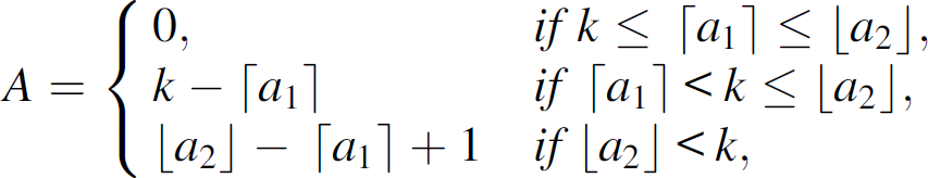
Let w be a prime such that w ≥ 2T − 1. Then the number of solutions (t, x) satisfying the equation

$$0<S^{\prime }\le txmodw\le S\le w-1$$

(8)

where, 0 < t ≤ T < w and 0 ≤ × ≤ X < w, is given by ${\sum }_{t=1}^T{\sum }_{t=0}^{t-1}{S}_1$ where u₁ = (wl + S′)/t, u₂ = (wl + S)/t and

$$S_1=\{\begin{array}{ll}0,& if\hspace{0.17em}X+1\le \lceil u_1\rceil \le \lfloor u_2\rfloor ,\\ X+1-\lceil u_1\rceil & if\hspace{0.17em}\lceil u_1\rceil <X+1\le \lfloor u_2\rfloor ,\\ \lfloor u_2\rfloor -\lceil u_1\rceil +1& if\lfloor u_2\rfloor <X-1.\end{array}$$

Proof

When t = 1, three conditions can arise.

Case (i): If X + 1 ≤ S′, then there are no values of x which satisfy (8).

Case (ii): If S′ < X + 1 ≤ S, x = S′, S′ + 1, S′ + 2, …, X satisfy (8). So there are X + 1 - S′ solutions.

Case (iii): If S ≤ X, × = S′, S′ + 1, S′ + 2, …, S satisfy (8). So there are S - S′ + 1 solutions.

When t = 2, three conditions can arise.

Case (i): If $X+1\le ⌈\frac{s^{\mathrm{\prime }}}{2}⌉$ , then there are no values of x which satisfy (8).

Case (ii): If $⌈\frac{s^{\mathrm{\prime }}}{2}⌉<X+1\le ⌊\frac{s}{2}⌋$ , then $x=⌈\frac{s^{\mathrm{\prime }}}{2}⌉,⌈\frac{s^{\mathrm{\prime }}}{2}⌉+1,...,X$ satisfy (8). So, there are $X+1-⌈\frac{s^{\mathrm{\prime }}}{2}⌉$ solutions.

Case (iii): If $⌊\frac{S}{2}⌋\le X$ , then $x=⌈\frac{S^{\mathrm{\prime }}}{2}⌉,⌈\frac{S^{\mathrm{\prime }}}{2}⌉+1,...,⌊\frac{S}{2}⌋$ satisfy (8). So there are $⌊\frac{S}{2}⌋-⌈\frac{S^{\mathrm{\prime }}}{2}⌉+1$ solutions.

When Case (iii) arises, then again consider the three sub cases.

Case (iii a): If $X+1\le ⌈\frac{w+S^{\mathrm{\prime }}}{2}⌉$ , then there are no values of x which satisfy (8).

Case (iii b): If $\lceil \frac{w+S^{\prime }}{2}\rceil <X+1\le \lfloor \frac{w+S}{2}\rfloor$ , then $x=\lceil \frac{w+S^{\prime }}{2}\rceil ,\lfloor \frac{w+S^{\prime }}{2}\rfloor +1,\cdots ,X$ satisfy (8).

So there are $\lfloor \frac{w+S}{2}\rfloor -\lceil \frac{w+S^{\prime }}{2}\rceil +1$ such solutions.

Case (iii c): If $\lfloor \frac{w+S}{2}\rfloor \le X$ , then $x=\lceil \frac{w+S^{\prime }}{2}\rceil ,\lceil \frac{w+S^{\prime }}{2}\rceil +1,\cdots ,\lfloor \frac{w+S}{2}\rfloor$ satisfy (8).

So there are $\lfloor \frac{w+S}{2}\rfloor -\lceil \frac{w+S^{\prime }}{2}\rceil +1$ such solutions.

Note that for $\lfloor \frac{S}{2}\rfloor <x<\lceil \frac{w+S^{\prime }}{2}\rceil$ , there is no solution when t = 2. The above cases give all the solutions when t = 2, since $\lceil \frac{lw+S^{\prime }}{2}\rceil >w,l>1$ . So, the number of solutions when t = 2, is ${\sum }_{l=0}^1{S}_1$ , where S₁ is as given.

Proceeding as above, t = m, three conditions can arise.

Case (i): If $X+1\le \lceil \frac{S^{\prime }}{m}\rceil$ , then there are no values of x which satisfy (8).

Case (ii): If $\lceil \frac{S^{\prime }}{m}\rceil <X+1\le \lfloor \frac{S}{m}\rfloor$ , then, $x=\lceil \frac{S^{\prime }}{m}\rceil ,\lfloor \frac{S^{\prime }}{m}\rfloor +1,\cdots ,X$ satisfy (8). So, there are $X+1-\lceil \frac{S^{\prime }}{m}\rceil$ solutions.

When Case (iii) arises, then again consider the three sub cases.

Case (iii a): If $X+1\le \lceil \frac{w+S^{\prime }}{m}\rceil$ , then there are no values of x which satisfy (8).

Case (iii b): If $\lceil \frac{w+S^{\prime }}{m}\rceil <X+\le \lfloor \frac{w+S^{\prime }}{m}\rfloor$ , then $x=\lceil \frac{w+S^{\prime }}{m}\rceil ,\lfloor \frac{w+S^{\prime }}{m}\rfloor +1,\cdots ,X$ satisfy (8). So there are $X-\lceil \frac{w+S^{\prime }}{m}\rceil +1$ such solutions.

Case (iii c): If $\lfloor \frac{w+S}{2}\rfloor \le X$ , then $x=\lceil \frac{w+S^{\prime }}{m}\rceil ,\lceil \frac{w+S^{\prime }}{m}\rceil +1,\cdots ,\lfloor \frac{w+S}{m}\rfloor$ satisfy (8). So there are $\lfloor \frac{w+S}{m}\rfloor -\lceil \frac{w+S^{\prime }}{m}\rceil +1$ such solutions.

Note that for $\lfloor \frac{S}{m}\rfloor <x<\lceil \frac{w+S^{\prime }}{m}\rceil$ there is no solution when t = m.

Again for Case (iii c), three cases can arise. Continuing similarly, we notice that if $\lfloor \frac{(m-2)w+S}{m}\rfloor \le X$ , the three conditions will arise.

Case (a): If $X+1\le \lceil \frac{(m-1)w+S^{\prime }}{m}\rceil$ , then there are no values of x which satisfy (8).

Case (b): If $\lceil \frac{(m-1)w+S^{\prime }}{m}\rceil <X+1\le \lfloor \frac{(m-1)w+S}{m}\rfloor$ , then $x=\lceil \frac{(m-1)w+S^{\prime }}{m}\rceil ,\lceil \frac{(m-1)w+S^{\prime }}{m}\rceil +1,\cdots ,X$ satisfy (8). So there are $X-\lceil \frac{(m-1)w+S^{\prime }}{m}\rceil +1$ such solutions.

Case (c): If $\lfloor \frac{(m-1)w+S}{m}\rfloor \le X$ , then $x=\lceil \frac{(m-1)w+S^{\prime }}{m}\rceil ,\lceil \frac{(m-1)w+S^{\prime }}{m}\rceil +1,\cdots ,\lfloor \frac{(m-1)w+S}{m}\rfloor$ satisfy (8). So there are $\lfloor \frac{(m-1)w+S}{m}\rfloor -\lceil \frac{(m-1)w+S^{\prime }}{m}\rceil +1$ such solutions.

Note that for $\lfloor \frac{(m-2)w+S}{m}\rfloor <x<\lfloor \frac{(m-1)w+S^{\prime }}{m}\rfloor$ , there is no solution when t = m. These are the only solutions when t = m, since $\lceil \frac{m^{\prime \prime }w+S^{\prime }}{m}\rceil >w$ , for m″ > m. So, the number of solutions when t = m, is ${\sum }_{l=0}^{m-1}{S}_1$ , where S₁ is as given.

Hence for all values of t, 1 ≤ t ≤ T, there are ${\sum }_{t=1}^T{\sum }_{t=0}^{t-1}{S}_1$ solutions satisfying (8).

We give the example given in [19] to demonstrate the above theorem. We consider the equation

$$0<txmod7\le 5\hspace{0.17em}and\hspace{0.17em}0<t\le 3\hspace{0.17em}and\hspace{0.17em}0\le x\le 4.$$

(9)

Note that w is a prime and w ≥ 2T − 1. For t = 1, the tuples (1, 1), (1, 2), (1, 3), (1, 4) satisfy (9). So, there are four solutions when t = 1. Here $\lceil u_1\rceil =1,\lfloor u_2\rfloor =5$ . Since 1 < X + 1 ≤ 5, from the formula in Lemma 1 there are $X+1-\lceil u_1\rceil =4+1-1=4$ solutions.

For t = 2, the tuples (2, 1), (2, 2), (2, 4) satisfy (9). So, there are three solutions when t = 2. When l = 0, ⌈u₁⌉ = 1, ⌊u₂⌋ = 2. Since X > 2, there are ⌊u₂⌋ + 1 − ⌈u₁⌉ = 2 + 1 − 1 = 2 solutions. When l = 1, ⌈u₁⌉ = 4, ⌊u₂⌋ = 6. Since ⌈u₁⌉ < X + 1 ≤ ⌊u₂⌋, there are X + 1 − ⌈u₁⌉ = 4 + 1 − 4 = 1 solutions.

For t = 3, the tuples (3, 1), (3, 3), (3, 4) satisfy (9). So, there are three solutions when t = 2. When l = 0, ⌈u₁⌉ = 1, ⌊u₂⌋ = 1. Since X > 1, there is ⌊u₂⌋ + 1 − ⌈u₁⌉ = 1 + 1 − 1 = 1 solutions. When l = 1, ⌈u₁⌉ = 3, ⌊u₂⌋ = 4. Since X ≥ ⌊u₂⌋, there are ⌊u₂⌋ − ⌈u₁⌉ = 4 − 3 + 1 = 2 solutions. When l = 2, ⌈u₁⌉ = 5, ⌊u₂⌋ = 6. Since X + 1 ≤ 5, there is no solution. All these three cases provide the overall count.

Using Lemma 1 and conditions (6a), (6b), (7a), and (7b) we arrive at the following theorem.

Theorem 1

$|A_p^{(i,j)}|=2\rho +2\sum _{t=1}^{\rho -1}(\sum _{t=0}^{t-1}A+\sum _{l=1}^{t}B)$ where, a₁ = (rl + 1)/t, a₂ = (rl + ρ - t)/t, b₁ = (rl − ρ + t)/t, b₂ = (rl − 1)/t, and

$$A=\{\begin{array}{ll}0,& if\hspace{0.17em}k\le \lceil a_1\rceil \le \lfloor a_2\rfloor ,\\ k-\lceil a_1\rceil & if\hspace{0.17em}\lceil a_1\rceil <k\le \lfloor a_2\rfloor ,\\ \lfloor a_2\rfloor -\lceil a_1\rceil +1& if\hspace{0.17em}\lfloor a_2\rfloor <k,\end{array}$$

and

$$B=\{\begin{array}{ll}0,& if\hspace{0.17em}k\le \lceil b_1\rceil \le \lfloor b_2\rfloor ,\\ k-\lceil b_1\rceil & if\hspace{0.17em}\lceil b_1\rceil <k\le \lfloor b_2\rfloor ,\\ \lfloor b_2\rfloor -\lceil b_1\rceil +1& if\hspace{0.17em}\lfloor b_2\rfloor <k,\end{array}$$

Proof

When x = 0, (i − 1, 0), (i − 2, 0), …, (i − ρ, 0) satisfy (6a).

For x ≠ 0, we can map (6a) to Lemma 1. Here, w = r, S′ = 1, S = ρ - t, T = ρ − 1, X = k − 1. So the number of solutions satisfying (6a) is given by $\rho +\sum _{t=1}^{\rho -1}\sum _{l=0}^{t-1}A$ . The number of solutions satisfying (6b) is given by $\sum _{t=1}^{\rho -1}\sum _{l=1}^{t}B$ .

Since we are considering the interior node, the number of key sharing neighbors in quadrant IV is the same as quadrant I and the number of key sharing neighbors in quadrant III is the same as quadrant II. Hence the total number of key sharing neighbors of n_{i, j} will be $2\rho +2\sum _{t=1}^{\rho -1}(\sum _{l=0}^{t-1}A+\sum _{l=1}^{t}B)$ . Hence the theorem.

Note that the value of $|A_{\rho }^{(i,j)}|$ from the above theorem and the value of $|B_{\rho }^{(i,j)}|$ from Eq. (2) directly provides the connectivity ratio $R_{\rho }^{(i,j)}=\frac{|A_{\rho }^{(i,j)}|}{|B_{\rho }^{(i,j)}|}$ for all interior node (i, j).

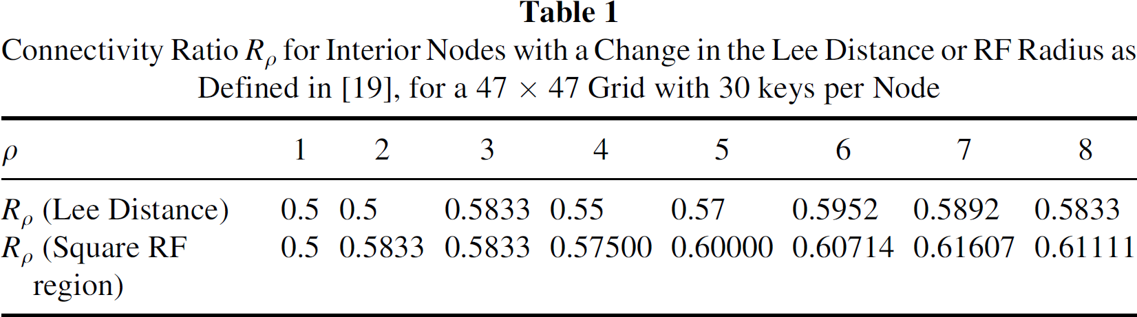
Table 1 compares the connectivity ratio with respect to the Lee sphere are square RF regions for an interior node. Though the connectivity ratio for square RF region is better we can see from the figures that Lee sphere is a better approximation of RF region. Figure 3 presents the connectivity ratio with varying k (the number of keys in each sensor). We see that as the number of keys increases, the connectivity ration increases.

Figure 3.

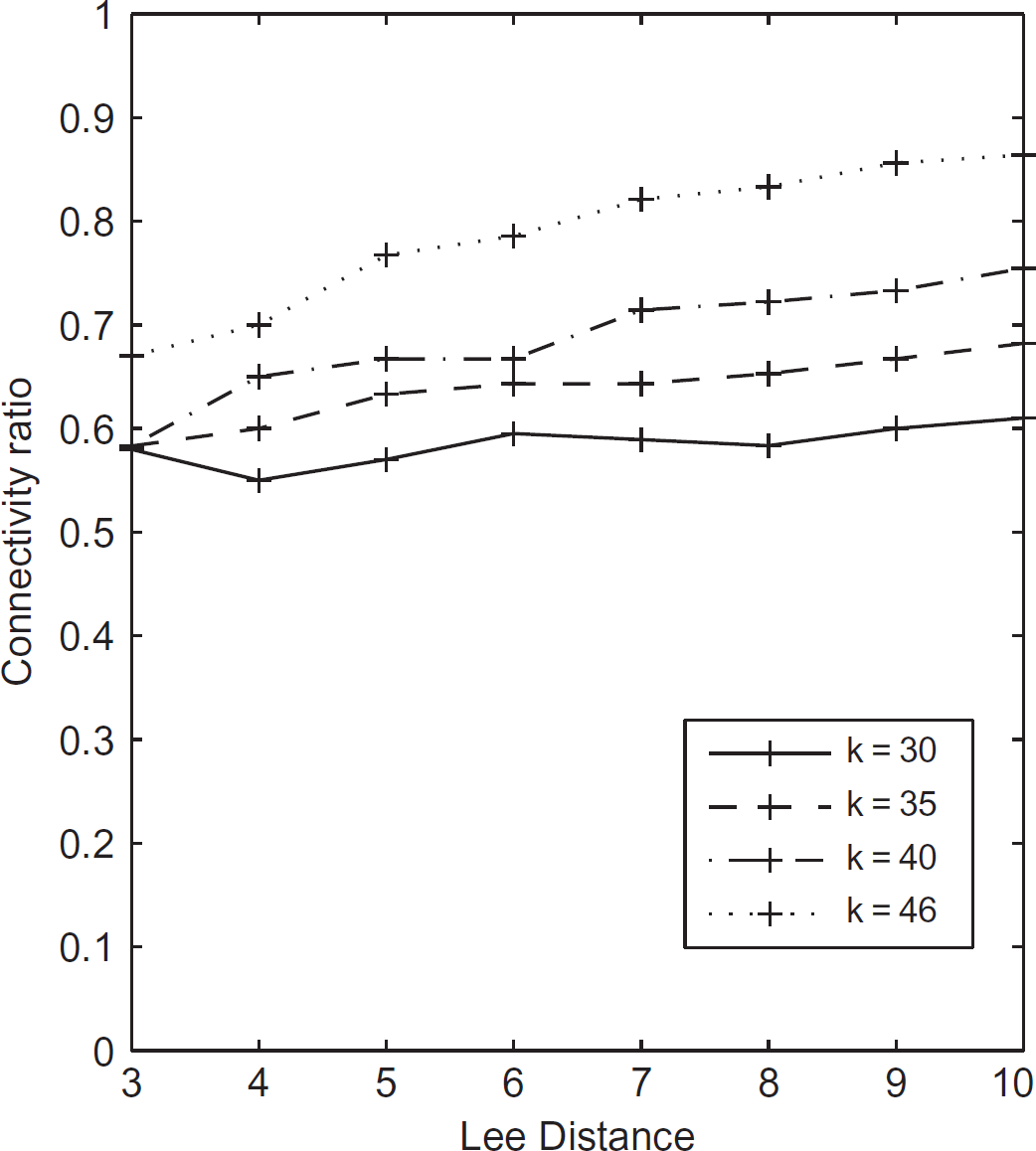
Comparison of connectivity ratio R_ρ with changing lee distance ρ and number of keys k on 47 × 47 grid.

Table 1

Connectivity Ratio R_ρ for Interior Nodes with a Change in the Lee Distance or RF Radius as Defined in [19], for a 47 × 47 Grid with 30 keys per Node

ρ	1	2	3	4	5	6	7	8
Rρ (Lee Distance)	0.5	0.5	0.5833	0.55	0.57	0.5952	0.5892	0.5833
Rρ (Square RF region)	0.5	0.5833	0.5833	0.57500	0.60000	0.60714	0.61607	0.61111

4. Resiliency

Sensor nodes are prone to failure and node capture or compromise. In case of node compromise, all the keys present in the compromised nodes are rendered ineffective. According to our design any two nodes share at most one common key. So all links which communicate via an exposed key are compromised (exposed). We give two parameters of resiliency of a Wireless Sensor Network (WSN), one based on the proportion of links that are broken and the other based on the proportion of nodes being disconnected.

E(s), which is defined as

$$E(s)=\frac{\text{Number of links exposed after}\hspace{0.17em}s\hspace{0.17em}\text{nodes are compromised}}{\text{Number of links present before compromise}}$$

V(s) which is the probability of a node (which is not among the compromised nodes) being disconnected when s nodes are compromised. A node (which is not among the compromised nodes) is considered disconnected if all the keys in the disconnected node are present in one or more compromised nodes.

We find an upper bound for E(s) and give some experimental results for V(s).

4.1. Estimation of E(s)

Let us denote the total number of links by T. Hence $T=\frac{1}{2}\sum _{i=0}^{r-1}\sum _{j=0}^{r-1}|A_{\rho }^{(i,j)}|$ .

There are a total of rk keys. If the nodes are compromised such that all rk keys are compromised, then all the links are broken. However, for simplicity we assume that only a small fraction of the nodes are compromised. Suppose s nodes are compromised. Maximum number of links are broken when the nodes compromised have disjoint sets of keys and occur in the interior.

Let the number of links broken when s nodes are compromised be denoted by C_s.

Consider a node n_i,j which has been compromised. Let it contain key (x, y). We find the nodes n_i′,j′ within Lee distance of n_i,j which share the key (x, y). By the analysis of $A_{\rho }^{(i,j)}$ , we see that the nodes n_i-1,j+x, n_{i-2,j+2x, …}, n _i-t,j+tx and n_i+1,j-x, n_{i+2,j-2x, …}, n_i+t,j-tx are the key sharing neighbors of the node n_i,j. So |t| ≤ ρ and either tx mod r ≤ ρ - t or r - |tx mod r | ≤ ρ - t. Since x is known, the number of nodes sharing key (x, y) within the Lee distance is the same as finding the number of values of t which satisfy the equations

$$|t|\le \rho \hspace{0.17em}\text{and}\hspace{0.17em}|txmodr|\le \rho -t$$

(10a)

and

$$|t|\le \rho \hspace{0.17em}\text{and}\hspace{0.17em}r-|txmodr|\le \rho -t$$

(10b)

We consider a key (x, y). Let us denote the number of links compromised when (x, y) is compromised is less than c_x. Let the following keys be exposed when s nodes are compromised. (x₁, y₁₁), (x₁, y₁₂) …, (x₁, y_1s1), (x₂, y₂₁), (x₂, y₂₂), … (x₂, y_2s2), …, (x_k-1, y_k-11), (x₁, y _5-12 ), …, (x₁, y_k-1sk-1). Each key occurs r times. So the number of links compromised is less than $r(\sum _{i=0}^{k-1}{c}_{x_i},s_i)$ . In reality the position of the compromised node and the position of the nodes which contain the exposed keys will determine the number of links compromised. Since the position of the nodes and the keys exposed cannot be determined, it is difficult to calculate an upper bound for the number of links exposed. $C_s\le r(\sum _{i=0}^{k-1}{c}_{xi}{s}_i).E(s)=\frac{C_s}{T}$ , where $T\le \frac{1}{2}\sum _{i=0}^{r-1}\sum _{j=0}^{r-1}|A_{\rho }^{(i,j)}|$ .

We give the experimental values of E(s) in Table 2.

Table 2

Experimental Value of E(s) for 100 Runs and Bound for E(s), when Number of Nodes in the Grid is r², Keys per Node is k and the Lee Distance (RF radius) is ρ

r	k	ρ	s	E(s) (Lee Distance)	E(s) (RF radius of [19])
23	15	7	5	0.1990	0.2006
23	15	5	5	0.1981	0.2008
31	20	7	5	0.1526	0.1516
31	25	7	5	0.1528	0.1513
37	30	7	5	0.1289	0.1283
53	49	7	5	0.0913	0.0915
53	49	7	10	0.1756	0.1736

4.2. Experimental Results for V(s)

V(s) can be defined as the probability that a node is disconnected, given that s nodes are compromised. Mathematically,

$$V(s)=\frac{\text{Number of nodes disconnected}}{r^2-s}.$$

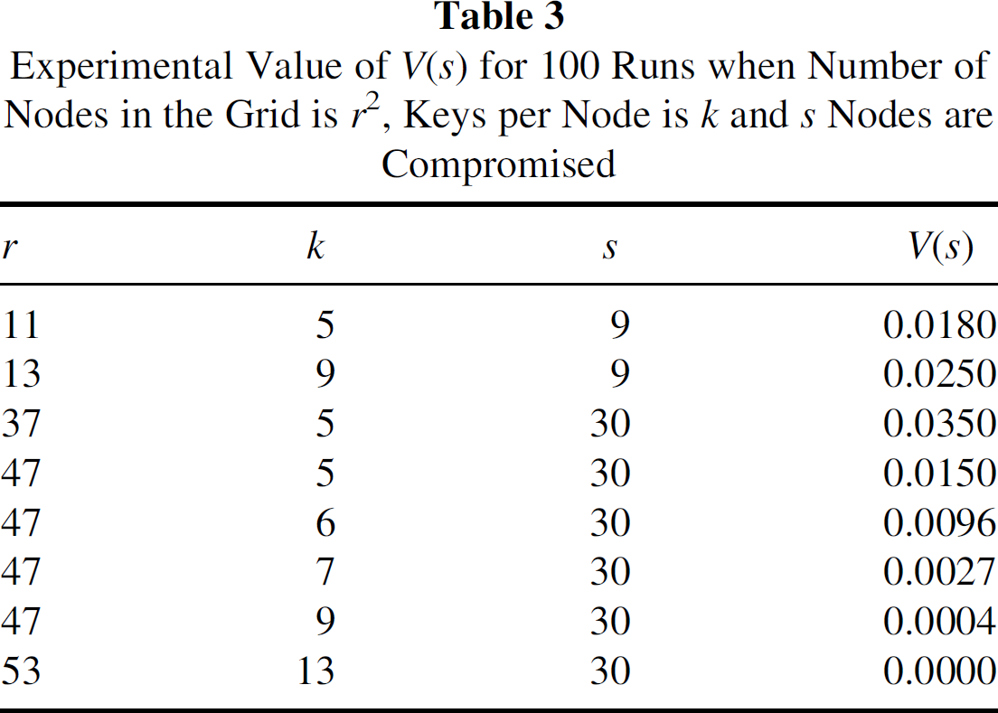
As discussed in [19] if s < k, no node is disconnected. For any node to be disconnected each of its k keys must be present in some compromised node. However, no two or more keys that are present in the disconnected node can be present in any compromised node, since any pair of nodes share at most one key. Hence there is no node which will have all the k keys in the compromised s sensor nodes.

Since the number of nodes disconnected when s nodes are compromised does not depend on the RF radius, we get the same results for V(s) as obtained in [19].

The experimental results for the calculation of V(s) is given in Table 3.

Table 3

Experimental Value of V(s) for 100 Runs when Number of Nodes in the Grid is r², Keys per Node is k and s Nodes are Compromised

r	k	s	V(s)
11	5	9	0.0180
13	9	9	0.0250
37	5	30	0.0350
47	5	30	0.0150
47	6	30	0.0096
47	7	30	0.0027
47	9	30	0.0004
53	13	30	0.0000

5. Related Works

Key predistribution using deployment knowledge has been studied in [1, 6, 7, 12, 15, 21, 28]. In this article, we use the Lee sphere approximation of RF region as discussed by Blackburn, Etzion, Martin, and Paterson in [1]. In [1] Blackburn, Etzion, Martin, and Paterson proposed a key predistribution scheme for a grid-based deployment scheme. They used combinatorial structures like Costas arrays and Distinct - difference configuration for key predistribution. However, their design is applicable, provided suitable Costas arrays and Distinct-difference configurations exist. The construction of Distinct-difference configuration which matches the desired requirements has not been presented in the paper. In our scheme all nodes are connected by a maximum of two-hop paths. However, using Costas arrays this is not guaranteed. (As the example of 3 × 3 Costas array in [1] shows.) Our design is simple and results in high resiliency in terms of V(s) and E(s) as already mentioned in the previous section. Though the number of groups is chosen to be r², where r is a prime power, the design discussed above works in all those cases where the dimension n of the grid is not a prime power. This can be done by simply choosing a prime power r > n and neglect the regions which fall out of the n × n grid.

6. Conclusion and Future Research

In this article, we revisit the grid-based deployment scheme as proposed by Ruj, Maitra, and Roy in [19]. Transversal designs are used for key predistribution. RF region is assumed to be a square of appropriate dimension in [19]. In [1] Blackburn et al. introduced Lee sphere as an approximation of the RF region. We use Lee distance while calculating the connectivity ratio and resiliency of the grid based network as proposed in [19]. The main reason for doing so is that Lee sphere provides a better approximation than the square RF region. This scheme is much better than the scheme proposed by Blackburn et al. mainly because it is very simple to construct transversal designs.

However, in the discussed key predistribution scheme a particular node may share keys with nodes which are not within its Lee distance. This is clearly a underutilization of resources. In future we would like to construct key predistribution schemes such that only nodes which are within Lee distance share keys with one another.