Sage Journals: Discover world-class research

Abstract

This article presents an algorithm for adaptive sensor activity scheduling (A-SAS) in distributed sensor networks to enable detection and dynamic footprint tracking of spatial-temporal events. The sensor network is modeled as a Markov random field on a graph, where concepts of Statistical Mechanics are employed to stochastically activate the sensor nodes. Using an Ising-like formulation, the sleep and wake modes of a sensor node are modeled as spins with ferromagnetic neighborhood interactions; and clique potentials are defined to characterize the node behavior. Individual sensor nodes are designed to make local probabilistic decisions based on the most recently sensed parameters and the expected behavior of their neighbors. These local decisions evolve to globally meaningful ensemble behaviors of the sensor network to adaptively organize for event detection and tracking. The proposed algorithm naturally leads to a distributed implementation without the need for a centralized control. The A-SAS algorithm has been validated for resource-aware target tracking on a simulated sensor field of 600 nodes.

Keywords

Wireless Sensor Networks (WSN)Sleep/Wake Scheduling Target Tracking Markov Random Fields Ising Model Self-Organization

1. Introduction

Recent advances in the technologies of microcomputers and wireless communications have enabled usage of inexpensive and miniaturized sensor nodes [1–3] that can be densely deployed in both benign and harsh environments as a sensor network for various applications. Distributed sensor networks have been built for both military (e.g., target tracking in urban terrain) and commercial (e.g., weather, habitat and pollution monitoring, and structural health monitoring) applications [4–8]. Sensor network operations can be broadly classified as:

(i)
data collection, and
(ii)
event detection and tracking.

Effective use of sensor networks requires resource-aware operation; once deployed, energy sources of sensor nodes can seldom be replenished. When used for data collection applications, sensor nodes are often operated on very low duty cycles (e.g., less than 1% [6]) to achieve appreciable operational lifetimes. Although several methods and design principles for power-aware communication and networking have been reported in recent literature [9, 10], the resulting communication strategies are more useful for low duty-cycle data collection applications because communication is the main source of energy consumption. Therefore, these methods may not be sufficient if the cost of sensing becomes significant relative to the cost of communications.

Sensor networks for event detection and tracking may not be able to afford a fixed low duty-cycle operation because events of interest are often rare and unpredictable. Therefore, sensor nodes need to be omni-active (i.e., (almost) always active), which makes the sensing task a significant contributor to the energy costs. A naive solution to this problem is to have a high duty cycle to achieve appreciable detection probability. Alternatively, a more sophisticated hierarchical approach (e.g., passive vigilance) may maintain a selected low-power sensor omni-active to trigger, as necessary, more energy-expensive sensors that are kept in standby modes [11]. This concept is valid if event detection is possible based only on the omni-active low-power sensor and the remaining sensors are required for further classification of the event/target. In many cases, successful event detection may require a high-power sensor or a combination of multiple sensors to be omni-active. An example is a combination of a low-power infrared sensor for line of sight together with audio and magnetic sensors for target tracking in an obstructed environment. However, such a configuration would significantly increase the power consumption. Energy costs for sensing are further aggravated and may prohibit continuous operation if active sensors (e.g., radio detection and ranging (radar) sensors [12]) are in use. In one such application, Arora et. al. [13] have used wireless sensor nodes equipped with a magnetometer and a micropower radar for detection and tracking on an experimental facility.

This paper presents an innovative algorithm to enable resource-aware operation for event detection and tracking. An adaptive sensor activity scheduling (A-SAS) algorithm is formulated based on the concepts drawn from Statistical Mechanics and random fields on graphs. The proposed A-SAS algorithm naturally leads to a distributed implementation on a sensor network and thus eliminates the need for a centralized control for sensor activity scheduling.

The rest of the paper is organized as follows. Section 2 provides the rationale and motivation for the presented work. The underlying problem is formulated in Section 3 and Section 4 presents the details of the methodology. Section 5 validates the proposed concept on a simulation test bed consisting of 600 sensor nodes. The paper is summarized and concluded with recommendations for future work in Section 6. Appendix A briefly introduces the measure-theoretic concept of a random field that has been used in the main body of the paper. Appendix B presents a comparison of Markov and Gibbs random fields.
2. Statistical Mechanics of Complex Networks

Recent literature in physics and related sciences suggests that there has been an increased interest in the interdisciplinary field of complex networks—found in diverse areas such as computer networks, sensor networks, social networks, biology, and chemistry. The unifying characteristic across various disciplines has been the fact that systems such as the internet and sensor networks can be described as a network of interacting complex dynamical systems. The major challenge while addressing the common issues in these systems is their high dimensionality and complex topological structures. This area has been traditionally investigated by using graph theory but recent work shows that tools of Statistical Mechanics facilitate understanding and modeling of the complex organizational characteristics in real-world complex networks. For example, by mapping nodes of a graph to energy levels and edges as particles occupying that energy level, Bianconi and Barabasi [14] have shown that complex networks follow Bose statistics and might undergo Bose-Einstein condensation despite their irreversible and non-equilibrium nature. In another article [15], Reichardt and Bornholdt have presented a fast community detection algorithm using a q-state Potts model. A detailed review of articles in this area can be found in [16, 17]. In this respect, the role played by Statistical Mechanics can be two-fold:

1)
Understanding the topological structures behind the multitude of networks, found in many real systems, whose structures lie in between a totally ordered one and completely disordered.
2)
Construction of algorithms, based on the above understanding, for control of local behaviors that through mutual interaction yield desired ensemble characteristics from a global perspective.

One of the important issues in the area of sensor networks is the judicious re-distribution of available resources such as energy and communication bandwidth. This paper makes use of the concepts of Statistical Mechanics and Markov Random Fields to formulate an Ising-like model of the sensor network. Ising's ferromagnetic spin model [18] has been used to study critical phenomena (e.g., spontaneous magnetization) in various systems. For example, its ability to model local and global influences on constituting units that make a binary choice (±1) has been shown to characterize the behavior of systems in diverse disciplines other than Statistical Mechanics, e.g., finance [19], biology [20], and sociophysics [21]. Markov random fields have been traditionally used for image processing [22], but their application to sensor networks [23], however, is a relatively new approach.

In this paper, a sensor network is modeled as a set of interacting nodes, where each node is modeled as a random variable with two states—active and inactive. A Hamiltonian based on clique potentials is constructed to model neighborhood interactions and time-dependent external influences. A sensor node recursively predicts the likelihood of being active or inactive based on perceived neighborhood influence and its most recently sensed parameters. Based on this likelihood, a sensor node probabilistically activates/deactivates itself while making only partial observations. Following the dynamics of a Markov random process, every sensor node makes local decisions that result in meaningful ensemble behaviors of the sensor network. This property is analogous to several multi-component systems such as those in finance and biology, where the collective behavior of the system emerges from the local decisions of interacting individual units that comprise it [24].
3. Problem Description

The problem addressed in this paper is to formulate a distributed algorithm for a sensor network to enable resource-aware detection and tracking of rare and random events. The task is to device entities (sensor nodes) that make local decisions leading to meaningful emergent behaviors of the sensor network. The sensor nodes are assumed to be equipped with relevant sensing transducers and data processing algorithms as needed for detection and tracking of events under consideration. Events (e.g., appearance of a target) occur in the sensor field at unpredictable locations and time instants, the task of the sensor network is to enable event detection and tracking while conserving resources. Sensor nodes can communicate with their nearest neighbors through single-hop wireless communications. The following assumptions are made to isolate the problem considered in this paper from other issues of a sensor network.

(i)
Once deployed, the nodes can localize themselves and discover their nearest neighbors.
(ii)
The sensor nodes considered are static. For a mobile or a hybrid (i.e., static + mobile)sensor network, periodic localization, and neighbor discovery would be required.
(iii)
Any communication to the data sink is handled by a dynamically selected cluster head [25] (see Algorithm 2 later in Section 5-B).
(iv)
Cluster heads talk to the data sink using short single-hop transmissions sending only filtered and fused information. It must be noted that this communication scheme is only a simplifying assumption and the proposed algorithm does not prohibit multi-hop transmission by the cluster head to the data sink.
(v)
Time synchronization is imperfect.

The accuracy of time synchronization is dictated solely by the required accuracy of event localization and the data aggregation for detection and tracking. Although interesting and challenging in their own right, issues such as localization, routing, and time synchronization in sensor networks are beyond the scope of this paper. An encompassing approach that factors in the details of all issues related to a sensor network is a topic of further research.
4. Algorithm Development

This section develops an algorithm of adaptive sensor activity scheduling (A-SAS) in distributed sensor networks, where the sensor network is modeled as a Markov random field on a graph. The sleep and wake modes of a sensor node are modeled as spins with ferromagnetic neighborhood interactions in the Statistical Mechanics setting.

4.1. Framework and Notations

This sub-section presents framework and notations that are used in further formulation. The sensor network is represented as a weighted graph. The choice of this framework is useful as it allows to model and utilize the dependence structure in a sensor network.

Let $G ≜ (S, E, W)$ be a weighted graph, where $S = {s_{1}, s_{2}, \dots, s_{N}}, N \in N$ is the set of all nodes of the sensor network under consideration; nearest (i.e., single-hop) neighbors are denoted by an edge (s_i, s_j) ∊ E which is a two-element subset of S representing communication and interdependence between nodes s_i and s_j; and the function $W : E \to R$ yields W((s_i, s_j)) = w_ij as the strength of interaction between the nodes s_i and s_j. The edges (s_i, s_j) or neighbor nodes are determined locally at each node. The strength of interaction w_ij is dictated by factors such as physical distance between the sensor nodes. Internode distance, for instance, can be locally determined by acoustic ranging using a sounder, an acoustic sensor and a radio [26]. A node emits a tone using its sounder and simultaneously sends an RF packet over the radio. Its neighbors assess the internode distance by estimating the time interval between the receipts of the RF packet and the acoustic tone. The graph $G$ is assumed to be undirected (i.e., symmetric interactions w_ij) and simple (i.e., no self-loops and no multiple edges between the same pair of nodes). However, in general, $G$ can potentially be a directed graph when the elements of E are 2-tuples and interactions between components are unsymmetrical.

It is noted that the graph $G$ , representing the sensor network, is not maintained as a whole at any central location. This framework is chosen only to facilitate further formulation. The algorithm eventually degenerates to localized computations with no need for a central controller for scheduling node activities.

4.2. Random Fields on Graphs

Let $F$ be a random field over the node set S defined as a family of random variables $F_{i}$ [27] (see Appendix A for details) as:

F = {F_{i} : Ω \to R^{d}, i = 1, 2, \dots, N}

(1)

where the random variable $F_{i} = F (s_{i}, ∙)$ is associated with the node s_i ∊ S and N = |S|. The sample space Ω of $F_{i}$ is the set of all states (or labels) that any node s_i can take. The cartesian product $K ≜ Ω^{N}$ is called the configuration space. A configuration $K \in K$ over the node set S is an ordered sequence (ω₁, ω₂,…, ω_N) of N states (or labels) with ω_i ∊ Ω being the state of a node s_i. The corresponding configuration $σ \in R^{N d}$ such that

σ = (σ_{1}, σ_{2} \dots, σ_{N}) = (F_{1} (ω_{1}), F_{2} (ω_{2}) \dots, F_{N} (ω_{N}))

(2)

with $σ_{i} \in R^{d}$ , is called a realization of the random field $F$ .

Definition 4.1 (Markov Random Field). Let $\partial ≜ {\partial_{i}}_{s_{i} \in S}$ be the neighborhood system, where ∂_i = {s_k : (s_i, s_k) ∊ E} is the neighbor set for a node s_i. Then, with respect to ∂ (or equivalently $G$ ), a random field is called a Markov Random Field (MRF) if and only if the following conditions hold [28]: 1)

Positivity: $P (K) > 0, \forall K \in K$

Markov Property: $P (ω_{i} | K_{S ∖ {i}}) = P (ω_{i} | K_{\partial_{i}})$

where K_S\{i} and K_∂i are configurations specified for the node set S\{i} and ∂_i respectively; P is the probability measure over the random field $F$ .

The first condition of positivity in Definition 4.1 ensures that the conditional probabilities P(ω_i|K_S\{i}) uniquely determine the joint probability P(K) [29]. The second condition of Markov property ensures that the probability of a node being in a state depends only on its neighbors (local property).

Definition 4.2 (Gibbs Random Field). A random field $F$ on a graph $G$ is called a Gibbs random field if the probability measure P on $F$ follows the Gibbs distribution¹ [28] given as:

P (K) = \frac{1}{Z_{N}} exp (- β H (K))

(3)

where

Z_{N} = \sum_{K \in K} exp (- β H (K))

(4)

is the partition function and β is the inverse temperature in the thermodynamic analogy.

For an uncountable Ω, the partition function Z_N becomes an integral, instead of the sum in Equation (4) for which Ω is finite or countably infinite. Moreover, for a countably infinite or an uncountable Ω, Z_N is defined only when the sum (or integral) in Equation (4) is finite [29]

Definition 4.3. A node set c ⊆ S is called a clique if the graph induced by $G$ on c is complete, i.e., if any two nodes in c are mutual neighbors in $G$ [31].

Definition 4.4. The Hamiltonian or the energy function for a configuration K is defined as:

H (K) = \sum_{c \in C} V_{c} (K)

(5)

where V_c is the potential of a clique c; and C is the set of all cliques for graph $G$ .

It is noteworthy that a Markov random field evolves as a localized process with neighborhood interactions only (i.e., Markov condition). In contrast, Gibbs random field describes global behavior relying on the joint probability measure P(K). Hammersley-Cliffford Theorem [28], [29] establishes an equivalence between Markov and Gibbs random fields (See Appendix B). Relying on this equivalence, the local behavior of a sensor node is tuned to achieve global emergent patterns for sensor activity scheduling.

4.3. Ising Model Formulation for a Sensor Network

This subsection formulates the Ising model of a sensor network, which is represented as a Markov random field on a graph $G$ . The rationale is that the behavior of a sensor node would depend strongly on its nearest neighbors and would be relatively unaffected by the decisions of a distant node. Sensor nodes are represented as binary random variables and clique potentials to model node behavior are defined. The goal here is to achieve desired sensor network activity through a distributed probabilistic approach as explained below.

A sensor s_i is represented as a function $s_{i} : P \to R^{n}$ that maps the physical space P of observable parameters into the measurement space $R^{n}$ . Often the attributes of a sensor data sequence - metadata - such as signal amplitude, frequency spectrum, wavelet coefficients, or their statistical signature, are used to create a scalar measure μ by comparing with known typical attributes for an event. This measure μ is then used for event detection and classification. For example, statistical feature extraction and information-theoretic approaches have been shown to create an anomaly measure for damage detection and tracking in electromechanical systems [32, 33]. Instead of directly incorporating sensor data sequences belonging to the space $R^{n}$ , construction of clique potentials for $G$ is based on such a scalar measure μ.

The state (or label) set is chosen to be discrete with Ω = {active, inactive}. The random field $F$ in Equation (1)) is defined as:

F_{i} : Ω \to {- 1, + 1}, \forall_{i} = 1, 2, \dots, N

(6)

with $F_{i} (a c t i v e) = + 1$ and $F_{i} (i n a c t i v e) = - 1$ for all i. In the Ising-mode analog {−1, +1} would correspond to the set of spins. Note that the number of possible configurations is |Ω|^|S| for a discrete Ω. Thus, even for a small label set and an appreciable size of the sensor network, |Ω|^|S| can be extremely large. The sensor network needs to be organized in configurations that enable detection and tracking while conserving resources as much as practicable. The proposed methodology achieves this objective by making use of a distributed approach that is computationally efficient.

The clique potentials are defined as

V_{c} = {\begin{cases} - B (μ_{i}^{τ}) σ_{i} & ; | c | = 1, s_{i} \in c \\ - w_{i j} σ_{i} {\hat{σ}}_{j} & ; | c | = 2, c = (s_{i}, s_{j}) \\ 0 & ; | c | > 2 \end{cases}

(7)

where |c| is the cardinality of the clique c; $μ_{i}^{τ}$ is the time τ-dependent scalar measure from node $s_{i}; B (μ_{i}^{τ})$ is an a priori defined function of $μ_{i}^{τ}$ ; and ${\hat{σ}}_{j}$ is the expected value of σ_j. The choice of the function $B (μ_{i}^{τ})$ and its effect on performance are discussed later in this section. Note that the clique potential for |c| = 2 is anisotropic² and V_c(σ_i, σ_j) ≠ V_c(σ_j, σ_i).

Cliques of size more than two would require keeping track of neighbors of neighbors, which becomes cumbersome for a large |c|. Therefore, from the implementation perspective, cliques with size greater than 2 are not considered in this formulation and hence V_c = 0 for |c| > 2. However, higher order cliques potentials are necessary in some scenarios for more complex sensor network behaviors; this is a topic of future research.

The Hamiltonian that represents the energy of a configuration K is now written in terms of the potentials V_c as:

H (K) = - \sum_{\begin{matrix} | c | = 1 \\ (c = s_{i}) \end{matrix}} B (μ_{i}^{τ}) σ_{i} - \sum_{\begin{matrix} | c | = 2 \\ (c = (s_{i}, s_{j})) \end{matrix}} w_{i j} σ_{i} {\hat{σ}}_{j}

(8)

where, in the Ising-model analogy, $B (μ_{i}^{τ})$ corresponds to the external magnetic field and w_ij to the coupling constant [18]. Each w_ij is assumed to be strictly positive, which is analogous to ferromagnetic influences in the thermodynamic sense [30]. That is, being in the same spin state as its neighbors is energetically favorable for a sensor node. However, due to the anisotropy of the clique potential, the interaction term in Equation (8) depends on the expected neighbor spin ${\hat{σ}}_{j}$ rather than its current value σ_j. This formulation has a practical significance from the perspectives of a sensor network. For example, the current value of σ_j for a neighbor could be unknown or erroneous due to data latency and simultaneous and unsynchronized operations of a sensor network. It is shown later in Equation (13) that the computation of state probabilities for a sensor node s_i is independent of the current state of its neighbors; this property enables nodes to make simultaneous transitions based on the expected neighbor behavior. Moreover, this formulation is meaningful even in the presence of a perfect (i.e., time-synchronized and zero latency) network. It allows a node to distinguish between a neighbor whose current state (possibly low probable) is a simple realization of the random variable σ_j, and one that has a bias towards certain state.

For a given configuration K, the conditional probability P(ω_i |K_S\{i}) (see Equation (3) and Equation (5)) is expressed as:

P (ω_{i} | K_{S ∖ {i}}) = \frac{exp (- β \sum_{c \in C_{i}} V_{c} (K))}{\sum_{ω_{i}^{'} \in Ω} exp (- β \sum_{c \in C_{i}} V_{c} (K^{'}))}

(9)

where C_i is the set of all cliques that contain the node s_i; and K′ is the configuration K with node s_i being labeled as $ω_{i}^{'}$ . The sum in the denominator is taken over all configurations K′ obtained with $ω_{i}^{'} \in Ω$ . (See Equation (22) in Appendix B for details).

Let ΔH(σ_i) be the change in energy as a node s_i changes its state from σ_i → − σ_i. Then,

\begin{aligned} Δ H (σ_{i}) & = H (K | ω_{i} = - σ_{i}) - H (K | ω_{i} = σ_{i}) \\ = 2 B (μ_{i}^{τ}) σ_{i} + 2 \sum_{s_{j} \in \partial_{i}} w_{i j} σ_{i} {\hat{σ}}_{j} \end{aligned}

(10)

Let $p_{j}^{a} ≜ P (σ_{j} = 1 | K_{S ∖ {j}})$ denote the conditional probability of the node s_j being active. Then, ${\hat{σ}}_{j} = 2 (p_{j}^{a} - \frac{1}{2})$ where the bias of the node s_j is clearly observed; and ΔH(σ_i) is expressed as:

Δ H (σ_{i}) = 2 B (μ_{i}^{τ}) σ_{i} + 4 \sum_{s_{j} \in \partial_{i}} w_{i j} σ_{i} (p_{j}^{a} - \frac{1}{2})

(11)

It follows from Equation (11) that ΔH(σ_i) = − ΔH(−σ_i), i.e., ΔH is an odd function of σ_i.

Setting $Δ H_{i} = Δ H (σ_{i}) |_{σ_{i} = - 1}$ for the node s_i, the state probabilities $(p_{i}^{a}, 1 - p_{i}^{a})$ are now expressed using Equation (9) as:

p_{i}^{a} = \frac{exp (- β Δ H_{i})}{1 + exp (- β Δ H_{i})}

(12)

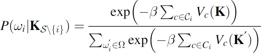
Both Equations (9) and (12) imply that P(ω_i|K_S\{i}) = P(ω_i|∂_i) and the computation of state probabilities require only local knowledge. Furthermore, partition function Z_N does not appear in the local computations.

Equations (12) and (11) together highlight the coupled nature of the node state probabilities as:

\frac{p_{i}^{a}}{1 - p_{i}^{a}} = exp (2 β B (μ_{i}^{τ}) + 4 β \sum_{s_{j} \in \partial_{i}} w_{i j} (p_{j}^{a} - \frac{1}{2}))

(13)

It is seen from Equation (13) that the probability of being active $p_{i}^{a}$ is a function of the current sensed parameters at the node s_i and the expected behavior of its neighbors. In the absence of the magnetic field $B (μ_{i}^{τ})$ that represents exogenous influences as a function of $μ_{i}^{τ}$ , the node probabilities depend only on the neighbors' behavior and the sensor network system has a fixed point at p∗ = 0.5, i.e., $p_{i}^{a} = p^{*} \forall i$ , both left hand and right hand sides of Equation (13) are identically equal to 1. This implies unbiased operation for all nodes.

The fixed point of the system determines the normal or usual operation characteristics of the system, i.e., when there are no events in the sensor field (μ_i = 0 ∀_i). Thus, for a sensor network application, the ability to choose p∗ would be desirable. For a given 0 < p∗ < 1, this is accomplished as follows.

Let us define the clique potentials as:

V_{c} = {\begin{cases} - (B_{0} + B (μ_{i}^{τ})) σ_{i} & ; | c | = 1, s_{i} \in c \\ - w_{i j} σ_{i} Δ {\hat{σ}}_{j} & ; | c | = 2, c = (s_{i}, s_{j}) \\ 0 & ; | c | > 2 \end{cases}

(14)

where

B_{0} = \frac{1}{2 β} ln (\frac{p^{*}}{1 - p^{*}})

(15)

and $Δ {\hat{σ}}_{j}$ is the change in the expected neighbor spin. For a given p∗, $Δ {\hat{σ}}_{j} = {\hat{σ}}_{j} |_{p_{j}^{*}} - {\hat{σ}}_{j} |_{p^{*}} = 2 (p_{j}^{a} - p^{*})$ . Then, Equation (13) becomes

\frac{p_{i}^{a}}{1 - p_{i}^{a}} = exp (β (2 B_{0} + 2 B (μ_{i}^{τ}) + 4 \sum w_{i j} (p_{j}^{a} - p^{*})))

(16)

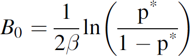
and the sensor network system has a fixed point at p∗ for μ_i = 0∀_i. In this model, a sensor node is allowed to make its local decisions based on its sensed parameters (μ_i) and the change $Δ {\hat{σ}}_{j}$ in the expected behavior of its neighbors. Note that, for p∗ = 0.5, Equation (16) degenerates to the earlier model in Equation (13).

The formulation presented here essentially follows a hybrid model [34] where the clique potentials and hence the probabilities are functions of both a discrete variable (σ_i) and a continuous variable ${\hat{σ}}_{j}$ . This model formulation is different from the conventional practice (e.g., auto-logistic and auto-normal models used in image processing) and has been adopted here to suit sensor network applications.

The schematic view in Fig. 1 represents a sensor network with orthogonal nearest neighbors. The network is perceived as a collection of interacting probabilistic finite state automata (PFSA). To adapt to the dynamic operational environment, sensors nodes recursively compute their state probabilities based on their neighborhood interactions and most recently sensed data. Although only two states (i.e., active and inactive) have been considered for each node, the formulation is extendable to a larger number of states (e.g., with a Potts model representation [18]) and is a topic of future research.

Figure 1

Sensor Field with sensor nodes represented as a probabilistic finite state automaton (PFSA) (magnified) with two states - Active (+1) and Inactive (−1), with p^a and (1 − p^a) as respective state probabilities.

5. Validation on a Simulated Sensor Field

Tests have been conducted on a simulated sensor field to demonstrate and validate the performance of the methodology presented above. The sensor field is simulated as a two-dimensional array of sensor nodes (like TelosB or MICAz [1, 2]). The sensor field consists of 600 (20 × 30) nodes which are placed in a uniform grid. Each node has four neighbors— nearest orthogonal, with inter-node distance between the neighbors being set to 10 units. Note that with nearest orthogonal neighbors, cliques of order three or more are not present. The scalar measure μ_i is taken to be the normalized signal intensity detected by the sensor node s_i. If the analysis based on mere intensity cannot be used for event detection, more advanced methods such as frequency domain, wavelet domain, or pattern recognition analysis would be required to compute the measure μ_i [32]. In the current simulation tests, $B (μ_{i}^{τ}) = B_{1} μ_{i}^{τ}$ is chosen to be a proportional function of $μ_{i}^{τ}$ and w_ij are chosen to be identical so that w_ij = w for all neighbor pairs (s_i, s_j).

Unlike a true spin system (e.g., a ferromagnet), information exchange between a pair of sensor nodes is possible only when both nodes in active state and communicating. A true spin system would correspond to a sensor network where nodes are always listening, so that any changes in the expected behavior of neighbors are promptly known. To this effect, algorithms (e.g., Low Power Listening (LPL) [35]) that offsets the load of communication to the transmitting node, can be utilized but they could be expensive. When not opting for such a communication scheme, a sensor node can only have a passive influence on its neighbors and therefore may not be able to actively update or wake-up a sleeping node. Using the last reported neighbor probabilities, a node handles the task of communicating to its neighbors as follows.

For a node s_i, let $p_{m} = min_{j} (p_{j}^{a}), j \in \partial_{i}$ where $p_{j}^{a} ≜ P (σ_{j} = 1 | K_{S ∖ {i}})$ denote the conditional probability of the node s_j being active as stated earlier in the previous section. Then, in a discrete time setting for time τ, the probability that the least probable neighbor would be active at least once in k time steps is 1 − (1 − p_m)^k.

Expiry time T_exp for broadcast is calculated so that P_comm = 1 − (1 − p_m)^Texp and thus

T_{exp} = \frac{ln (1 - P_{comm})}{ln (1 - p_{m})}

(17)

where P_comm is a design parameter that determines the likelihood of updating one's neighbors and thus T_exp, as seen in Fig. 2. Thus, a sensor node broadcast new $p_{i}^{a}$ for broadcast expire time T_exp, to update its least active neighbor with probability P_comm. Nodes broadcast new pa only when it changes by δp^a. This is done so that insignificant changes in p^a are not broadcast.

Figure 2

Trend of the design parameter P_comm versus time steps k.

Sensor network activity is scheduled via a stochastic update of node states, as given in Algorithm 1. In a discrete time setting, a node s_i computes $p_{i}^{a}$ at each time step k based on its current $μ_{i}^{k}$ and last known neighbor probabilities $p_{j}^{a}, j \in \partial_{i}$ . It then assigns a state active or inactive to itself for this time step with probability $p_{i}^{a}$ and $(1 - p_{i}^{a})$ respectively. These stochastic local decisions, in turn, evolve to adapt to the changing environment. The following subsection present results from two simulation experiments: 1)

The effects of neighborhood interactions on sensor network performance (see Subsection 5.1), and

A target tracking application (see Subsection 5.2).

5.1. Neighborhood Interactions

Neighborhood interactions in the proposed methodology enable a sensor node to adapt its activity schedule to an event in its vicinity. This event may not be directly visible to the sensor node. To demonstrate the effects of neighborhood interaction, an event is simulated to be detected by only one sensor node (i.e., s₀ at grid point (15,10) in Fig. 3). This is done by setting μ₀ = 1 for node s₀ and μ_i = 0 for all nodes s_i, i ≠ 0. Figure 3 shows six contour plots, (a) to (f), of activity probability p^a of sensor nodes for w = 0, 0.8, 1.2, 1.35, 1.8, and 2.0 respectively. For all six cases (a) to (f), fixed point p∗ = 0.3, β = 0.2 and parameter B₁ = 50.

Figure 3

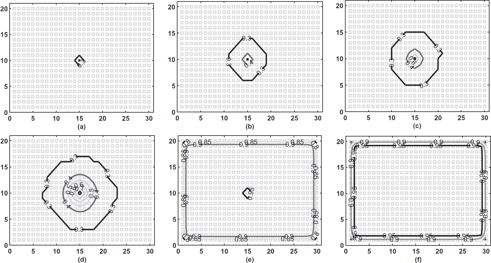
Contour plots of activity probability p^a of sensor nodes when for different values of w: (a) w = 0, (b) w = 0.80, (c) w = 1.20 (d) w = 1.36, (e) w = 1.80 and (f) w = 2.0. Only one sensor at grid point (15,10) is detecting the event. (p∗ = 0.3).

As explained in Section 4.3, in the absence of an event each sensor node operates at the fixed point with p^a = p∗. But when an event gets detected by a sensor node, each node adjusts its activity probability p^a thorough local decisions to adapt to the changes in the environment. This can be seen in the contour plots in Fig. 3. For w > 0 sensor nodes in the immediate neighborhood of grid point (15,10) achieve higher probability of activity through local interactions although they are unable to detect the event directly. This influence gradually decreases further away from the node s₀, which is detecting the event.

In Fig. 3 the contour line for p^a = 0.3 = p∗ can be considered as the boundary of the influence patch due the event at s₀. Cases (b), (c), and (d) for w = 0.8, 1.2, and 1.36 respectively show that nodes far away from s₀ remain undisturbed by the event and operate at the fixed point p∗ of the network. Although, the size of the influence patch grows with increase in w. In case (e) and (f) where w = 1.8 and 2.0 respectively, the event at s₀ can be seen to influence the entire network and a large number of nodes have a high probability of being active.

Figure 4 shows a plot of expected number of active nodes $n_{a} (= Σ_{i} p_{i}^{a})$ with interaction coefficient w. The simulation was repeated fives times for each value of w and the value n_a of the sum $Σ_{i} p_{i}^{a}$ was recorded when it stabilized within an error bound (10⁻²). Expected number of active nodes for each run are marked as ∗ in Fig. 4, while the solid line shows the average trend of the simulation data points. Figure 4 shows that there is a sudden change in behavior of the sensor network at w = 1.36. For w ≤ 1.36 the n_a has a low value (≈180 for w = 0)³, and shows a slow rise changing only by a small number of nodes. For w > 1.36, expected number of active nodes jumps to high value (>400) and rises quickly as w is increased. For w = 3 almost all nodes (≈600) achieve pa close to unity. This abrupt change or discontinuity in n_a can be seen as a phase change of zeroth order in the thermodynamic sense. The value of w is stepped by 0.2, except around w = 1.36 where it is stepped by 0.02 to adequately characterize the discontinuity in n_a.

Figure 4

Expected number of active nodes $(\sum p_{i}^{a})$ with respect to w for β = 0.2.

Results show that neighborhood interaction allows sensor nodes to gradually adapt to an event even before it gets directly detected by them. These interactions lead to the formation of an influence patch whose size can be controlled using an appropriate choice of w. Above the critical point, a localized event detected by single node can activate a large number of nodes. Thus, to ensure a stable performance of the sensor network operating below the critical point is desirable. It should be noted that the critical point for phase transition is dependent on the inverse temperature β.

5.2. Target Tracking

This section presents a target tracking application of the proposed methodology. The intensity of the signal, used to detect the target, is simulated to follow inverse-square law. This would be true in many cases such as when the target has an acoustic or a magnetic footprint. In both cases the signal intensity would decay proportional to r⁻², where r is the distance form the target. An acoustic response from the target would be obtained when a noisy target moves through the sensor field. While, ferrous targets such as a vehicle would produce a magnetic signature by affecting the nearby Earth's magnetic field.

The task of estimation of target attributes such as position and communication to the data sink is handled by cluster head. Dynamic Space-Time Clustering (DSTC) given in Algorithm 2 [25] is used by the sensor nodes to elect cluster heads. Cluster heads perform local information fusion and transmit assimilated data as short packets to the data sink using single-hop communication. In the current work cluster heads estimate the position of the target using a weighted mean of sensor node positions. The weights used are the corresponding measures μ_i from the sensor nodes. The data sink may receive data from one or more cluster heads and use it to get a final estimate of the target position. Cluster head selection, target position estimation, and communication to a data sink are done to demonstrate efficacy of the proposed methodology to enable target tracking. A more sophisticated approach such as multilateration or Kalman filtering for position estimation can be used. Sensor field is the same as used for studying the effect of neighborhood interaction.

Algorithm 1

Adaptive Sensor Activity Scheduling (A-SAS)

Algorithm 2

Electing Cluster Head

Figure 5 shows the results for target tracking as snap shots at three instants of time - cases (a), (b), and (c). Each case shows the sensor field and a contour plot. The sensor field shows the sensor nodes in four modes - (i)

active (sensing and sniffing for messages from neighbors - Rx),

(ii)

inactive (neither sensing nor receiving),

(iii)

cluster head (performing information fusion besides sensing and receiving) and (iv) transmitting (sending new p^a to neighbors - Tx).

Figure 5

Snap shots of the sensor field and activity probability p^a contour plots. Subplots (a), (b) and (c) show three positions of the target progressively advanced in time. (p∗ = 0.3).

The corresponding contour plots show the distribution of activity probability p^a of sensor nodes. It can be seen that as the target moves through the sensor field, sensor nodes adapt their p^a to suit the current scenario. The contour plots show that the target (black dot) is always in an area of high probability of activity. While sensor nodes far away are unaffected by the presence of the target. This is confirmed by the snap shot of the sensor field, which shows nodes in the immediate neighborhood of the target in active mode and elected as cluster heads for information fusion. Nodes ahead of the target are transmitting to inform neighbors of their current (increase in) probability. While nodes behind the target are informing their neighbors of new p^a (decreased as target moved away).

As for previous application, measure μ_i is taken as the normalized signal intensity. Parameters p∗, β, w and B₁ are chosen as 0.3, 0.2, 0.8, and 10. In Algorithm 2 p_c = 0.9 for cluster head election and change in activity probability δp^a = 0.02 in Algorithm 1 to broadcast p^a to neighbors. Nodes transmit for a period T_exp (Equation (17)) to ensure with P_comm = 0.95 likelihood that their least active neighbors receive their messages. Note that T_act and T_inact in Algorithm 1 are the time durations for active and inactive states respectively. They have been chosen to be unity in both simulations. Their choice would dependent on the application at hand.

Figure 6 show the true track of the target (solid line) and the estimate of its position obtained using the weighted mean approach. Estimated target positions are appreciably close to the true target track for a simple weighted mean approach. It can be seen that the sensor network is able to adaptively activate node so as to enable target tracking.

Figure 6

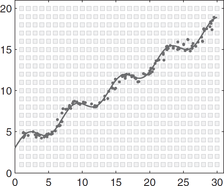
True target track (solid line) and estimated positions (dots) of the target obtained using weighted mean approach.

6. Summary, Conclusions, and Future Work

This paper presents an adaptive methodology for sensor node activity scheduling in sensor networks based on the fundamental concepts of random fields on graphs and Statistical Mechanics. Clique potentials have been defined in this context and a hybrid Ising-like model is constructed to suit a sensor network application. This procedure allows the sensor nodes to make simultaneous local decisions by relying on their sensed parameters and changes in expected behavior of their neighbors. These local decisions, in turn, evolve to a meaningful global behavior of the sensor network. Tests have been conducted on a simulated sensor field of 600 nodes to (i)

observe the effects of neighborhood interactions and

(ii)

for a target tracking application.

The framework presented in this paper provides a method for collaboration in a sensor network for a resource aware operation. The following are a few directions for further investigation.

Extension to address situations where sensor node states are not binary;

Inclusion of factors such as communication link or sensor node reliability and inter-node distance in the interaction coefficient w_ij;

Use of methods such as statistical pattern recognition for the scalar measure μ [32], [33]; and

Stability control

Footnotes

1

Known as generalized canonical distribution in Statistical Mechanics, where it is derived as an unbiased distribution of microstates subject macroscopic observations, such as energy [].

2

A clique potential is called anisotropic (isotropic) when it is dependent (independent) of the clique orientation [].

3

For w = 0, $p_{i}^{a} = p^{*} = 0.3$ for all i ≠ 0 and $p_{0}^{a} \approx 1$ for node s₀. Thus $n_{a} = Σ_{i} p_{i}^{a} \approx 180$ .

Appendix

This appendix presents a more detailed and rigorous background on the theory of random fields used for methodology formulated in the main text.

References

Polastre

Szewczyk

Culler

D. E.

, “Telos: enabling ultra-low power wireless research.” in IPSN, 2005, pp. 364–369.

Hill

J. L.

Culler

D. E.

, “Mica: A wireless platform for deeply embedded networks,” IEEE Micro vol. 22, no. 6, pp. 12–24, 2002.

Phoha

LaPorta

T. F.

Griffin

, Sensor Network Operations. Wiley-IEEE Press, 2006.

Kim

Pakzad

Culler

Demmel

Fenves

Glaser

Turon

, “Wireless sensor networks for structural health monitoring,” in SenSys ′06: Proc. of the 4th intl. conf. on embedded networked sensor systems. New York, NY, USA: ACM, 2006, pp. 427–428.

Brooks

Friedlander

Koch

Phoha

, “Tracking multiple targets with self-organizing distributed ground sensors,” J. Parallel Distrib. Comput., vol. 64, no. 7, pp. 874–884, 2004.

Szewczyk

Osterweil

Polastre

Hamilton

Mainwaring

Estrin

, “Habitat monitoring with sensor networks,” Commun. ACM, vol. 47, no. 6, pp. 34–40, 2004.

Yang

Ong

K. G.

Dreschel

W. R.

Zeng

Mungle

C. S.

Grimes

C. A.

, “Design of a wireless sensor network for long-term, in-situ monitoring of an aqueous environment,” Sensors, vol. 4, no. 11, pp. 455–472, Nov 2002.

Akyildiz

Sankarasubramaniam

Cayirci

, “Wireless sensor networks: a survey,” Computer Networks, vol. 38, no. 4, pp. 393–422, Mar 2002.

Heidemann

Estrin

, “An energy-efficient MAC protocol for wireless sensor networks,” INFOCOM 2002. Twenty-First Annual Joint Conference of the IEEE Computer and Communications Societies. Proceedings. IEEE, vol. 3, pp. 1567–1576 vol.3, 2002.

10.

Shi

Stromberg

, “Syncwuf: An ultra low-power MAC protocol for wireless sensor networks,” Mobile Computing, IEEE Transactions, vol. 6, no. 1, pp. 115–125, Jan 2007.

11.

Dutta

Grimmer

Arora

Bibyk

Culler

, “Design of a wireless sensor network platform for detecting rare, random, and ephemeral events,” in IPSN ′05: Proceedings of the 4th International Symposium on Information Processing in Sensor Networks. Piscataway, NJ, USA: IEEE Press, 2005, p. 70.

12.

Ditzel

Elferink

, “Low-power radar for wireless sensor networks,” Radar Conference, 2006. EuRAD 2006. 3rd European, pp. 139–141, Sept. 2006.

13.

Arora

Dutta

Bapat

Kulathumani

Zhang

Naik

Mittal

Cao

Demirbas

Gouda

Choi

Herman

Kulkarni

Arumugam

Nesterenko

Vora

Miyashita

, “A line in the sand: a wireless sensor network for target detection, classification, and tracking,” Computer Networks, vol. 46, no. 5, pp. 605–634, December 2004.

14.

Bianconi

Barabási

A.-L.

, “Bose-einstein condensation in complex networks,” Phys. Rev. Lett., vol. 86, no. 24, pp. 5632–5635, June 2001.

15.

Reichardt

Bornholdt

, “Detecting fuzzy community structures in complex networks with a Potts model,” Phys. Rev. Lett., vol. 93, no. 21, p. 218701, Nov 2004.

16.

Albert

Barabási

A.-L.

, “Statistical mechanics of complex networks,” Rev. Mod. Phys., vol. 74, no. 1, p. 47, 2002.

17.

Strogatz

, “Exploring complex netwoks,” Nature(London) vol. 410, pp. 268–276,March 2001.

18.

Huang

, Statistical Mechanics, 2nd ed. New York, NY, USA: John Wiley, 1987.

19.

Greco

Carbone

Sorriso-Valvo

, “Non-poisson intermittent events in price formation in a Ising spin model of market,” Physica A: Statistical Mechanics and its Applications, vol. 376, pp. 480–486, March 2007.

20.

Bakk

Høye

, “One-dimensional Ising model applied to protein folding,” Phys. A, vol. 323, no. 1–4, pp. 504–518, 2003.

21.

Indekeu

, “Special attention network,” Physica A: Statistical Mechanics and its Applications, vol. 333, pp. 461–464, February 2004.

22.

Besag

, “On the statistical analysis of dirty pictures,” Journal of the Royal Statistical Society. Series B (Methodological), vol. 48, no. 3, pp. 259–302, 1986. [Online]. Available: http://www.jstor.org/stable/2345426.

23.

Brooks

Pirretti

Zhu

Iyengar

, “Distributed adaptation methods for wireless sensor networks,” Global Telecommunications Conference, 2003. GLOBECOM ′03. IEEE, vol. 5, pp. 2967–2971 vol.5, 1–5 Dec. 2003.

24.

Haken

, Information and self-organization, 3rd ed. Springer, 2006.

25.

Phoha

Koch

Grele

Griffin

Madan

, “Space-time coordinated distributed sensing algorithms for resource efficient narrowband target localization and tracking,” International Journal of Distributed Sensor Networks, vol. 1, no. 1, pp. 81–99, 2005.

26.

Girod

Estrin

, “Robust range estimation using acoustic and multimodal sensing,” Intelligent Robots and Systems, 2001. Proceedings. 2001 IEEE/RSJ International Conference on, vol. 3, pp. 1312–1320 vol.3, 2001.

27.

Alder

R. J.

, The Geometry of Random Fields. New York, NY: John Wiley & Sons, 1981.

28.

Grimmett

G. R.

, “A theorem about random fields,” Bull. London Math. Soc., vol. 5, no. 1, pp. 81–84, 1973. [Online]. Available: http://blms.oxfordjournals.org.

29.

Besag

, “Spatial interaction and the statistical analysis of lattice systems,” J. Royal Statistical Society, B, vol. 36, no. 2, pp. 192–236, 1974.

30.

Beck

Schlogl

, Thermodynamics of Chaotic Systems: An Introduction. United Kingdom: Cambridge University Press.

31.

West

D. B.

, Introduction to Graph Theory, 2nd ed. Prentice Hall, 2000.

32.

Ray

, “Symbolic dynamic analysis of complex systems for anomaly detection,” Signal Processing, vol. 84, no. 7, pp. 1115–1130, 2004.

33.

Srivastav

Ray

Gupta

, “An information-theoretic measure for anomaly detection in complex dynamical systems,” Mechanical Systems and Signal Processing, vol. 23, no. 2, pp. 358–371, 2009.

34.

Bouthemy

Hardouin

Piriou

Yao

, “Mixed-state auto-models and motion texture modeling,” J. Math. Imaging Vis., vol. 25, no. 3, pp. 387–402, 2006.

35.

Polastre

Hill

Culler

, “Versatile low power media access for wireless sensor networks,” in SenSys ′04: Proceedings of the 2nd International Conference on Embedded Networked Sensor Systems. New York, NY, USA: ACM, 2004, pp. 95–107.

Adaptive Sensor Activity Scheduling in Distributed Sensor Networks: A Statistical Mechanics Approach

Abstract

Keywords

1. Introduction

4.1. Framework and Notations

4.2. Random Fields on Graphs

Footnotes

1

2

3

Appendix

References