Sage Journals: Discover world-class research

Abstract

In general, wireless sensor networks have a certain degree of spatial redundancy, which means that a high number of nodes can sense the same event at the same time. This redundancy permits to simplify both MAC protocol and the transport of sensed data. In particular, in this paper, we review a widely accepted transport technique which makes use of the event-reliability concept. A system implementing this technique is essentially a control system, where the controlled variables are the reporting rates of sensor nodes and the control variable is a function of the perceived event reliability at the sink node. As control system, we are interested in stable operating points. If we respect the capacity limit of the network, such stable points exist. However, if we take into account also the irregularities of radio links, well documented in recent measurements on real sensors testbeds, possible unstable states may arise. Here, we study this problem by means of simulation of a wireless sensor network under the assumption of two simplified versions of the radio model. We found that indeed the routing protocols should be carefully engineered in order to support event reliability based techniques.

Keywords

Wireless Sensor Networks Data Transport Multi-hop Networks Event Detection Distortion Stability ns-2 Simulations Path stability Shadowing

1. Introduction

A Wireless Sensor Network (WSN) is a wireless network where nodes are sensors, that is micro-devices with limited computation capacity and with on-board specific transducers. These networks have been using in several application fields, e.g. the detection of a physical phenomenon as the temperature or the pressure, the detection and tracking of mobile objects. Recently, we witnessed a lot of research effort towards the optimization of standard communication paradigms for such networks. In fact, in the traditional Wireless Network (WN) constraints such as the limited or scarce energy of nodes and their computational power are not of concern. For example, we can afford to buy a cellular phone of more than hundred dollars and we can easily recharge its batteries. Another aspect which is different in traditional WNs is the communication reliability and congestion control. In traditional wired nets, one reasonably supposes that communication paths are stable along the transmission instances. This fact permits to use the end-to-end approach to the design of reliable transports and application protocols. The TCP works well because of the stability of links. On the other hand, in WSN paths can change over time, because of time-varying characteristics of links and nodes reliability as well. These problems are important especially in a multi-hop scenario, where nodes act also as relaying nodes. A failure of a link, caused by a node failure or by deep fade of the radio medium, triggers a new route discovery process. In a WSN, one has also to face the packet loss which is not negligible. In general, in WNs the cause of packet losses is the contention of the radio medium, the fading of the radio channel, and the buffer overflow of nodes which store and forward packets towards the destination. The radio channel contention arises when many source nodes try to access at the same time the same radio resource. This problem is solved by MAC protocol which controls the access rate to the channel in order to minimize packet collision, like the Distributed Coordination Function (DCF) of the IEEE 802.11 protocol, which is a CSMA/CA MAC protocol. Other MAC protocols are based on spatial-TDMA, where the nodes are assigned a time-slot in a distributed fashion. Spatial-TDMA techniques reduces contention and improves network throughput, but they may suffer other problems, such as the need of a distributed and global synchronization mechanism, the vulnerability to interference from other non-neighbouring nodes, and the periodic exchange of time-slot access information among neighboring nodes. For a review of the state-of-art on MAC protocols for WSNs, the reader can see [5]. However, in WSNs it has been shown that the packet loss shows also a strange correlation with the distance, and in general the packet loss is a time-varying process [15, 3]. This phenomenon should be taken into account in designing ad-hoc routing protocols for WSNs. Another characteristic of WSNs is their spatial redundancy. In a hypothetical architecture of a WSN for event detection, the sensor nodes are deployed in a certain area to detect some particular phenomenon. In such a WSN, there is always at least one sink node which collects data from sensor nodes. In a large WSN used to detect events, it is reasonable to assume that the number of sensor nodes which detect the event is higher than that strictly required. But, the sink node does not require that all the sensed data be transmitted, only a certain number of packets is enough in order to reconstruct reliably the event-field. This observation has stimulated the design of new MAC protocol for WSNs, which exploits the spatial redundancy in order to minimize packet collision, simplify the access to the medium, and conserve energy [7]. For example, in [11] the authors propose to use a nonpersistent CSMA/p* protocol with nonuniform access probability. The event-driven approach can be used also to simplify the transport of event data. In fact, by assuring that the distortion of the estimated event-field is minimized, not all the data are necessary. An example of this approach is the Event-to-Sink Reliable Transport (ESRT) proposed in [2]. The authors analyze a WSN aimed at the tracking of a particular physical phenomenon. They propose to use a control loop between the sink node and the network, in order to maximize the metric referred to as normalized reliability. This metric depends on the application, and in general it is a function of a detection interval. The event-reliability permits to tolerate at a certain extent the packet loss, because of the presence of redundant nodes. Therefore, we can use a simple connectionless transport for the transmission of the sensed data. The rate of the transmitted data depends on many factors, such as the bound on the signal distortion perceived at the sink node. This scheme resembles the packet repetition scheme, in the case of a discrete event in the form of “event present” or “event not present.”

Here, we analyse the impact of the radio links irregularities on the performance of the scheme. Recently, the importance of considering links irregularities has been shown to be a key system parameter in order to obtain accurate performance evaluations of WSNs [16]. To the best knowledge of the authors this fact is not taken into account in previous research on WSNs simulations for even-detection. The work in [12] addressed a similar technique, but in that work the objective was the understanding of the interdependency between losses caused by collision and congestion. The effects of the irregularities of radio link have not been considered, or at least underestimated. Here, we consider two simple models for the radio medium as “seen” by the sensor nodes. The first one is based on the shadowing assumption for the path loss between two nodes. Since this assumption could be unrealistic in some scenarios, we also consider a second model, where links suffer a certain packet loss. In both models, the links becomes asymmetric, i.e. the packet loss rate at a given node is not the same for incoming and outcoming packets. Given a system parameters set, it is clear that the stability of such a technique depends on the network throughput, that is the mean number of packets which can be delivered back to the sink node in a given detection interval. In fact, it might happen that the system is unable to find a stable point, by oscillating between low reliability states and high congestion states. We show how the irregularity of the radio medium affects the stability of the event-detection approach. In this view, ad-hoc routing and MAC protocols should be carefully engineered in order to accommodate the requirements of the WSN.

The paper is organized as follows. In Sections 2 and 3, we explain the model of WSN under test and the event detection/transport technique, respectively. In Section 4, we discuss the simulation results. Conclusions of the paper are given in Section 5.

2. WSN Model

In our WSN, every node detects the physical phenomenon and sends back to the sink node data packets. We suppose that the sink node is more powerful than sensor nodes and it is always located at the borders of the service area. This model can be considered as a model for remote monitoring of hazard or inaccessible areas [13]. We analyse the performance of the network in a fixed time interval, τ. This interval can be considered as the available time for the detection of the phenomenon and its value is application dependent.

2.1. Topology

For the physical layout of the WSN, two types of deployment have been studied so far: the random and the lattice deployment. In the former, nodes are supposed to be uniformly distributed inside the service area, while in the latter nodes are vertexes of particular geometric shape, e.g. a square grid. For space constraints, we present results for the square grid topology only. In this case, in order to guarantee the connectedness of the network we should set the transmission range of every node to the step size, d, which is the minimum distance between two rows (or columns) of the grid. In fact, by this way the number of links that every node can establishe, a.k.a the node degree is D = 4, if we do not count the nodes at the borders, which have D = 2 or D = 3. Let us note, that, by using Cooper's theorem [4] along with some power control techniques, D = 2 is enough to guarantee a connected network¹. The settings of our lattice are shown in Table 1. The network is supposed to have a single sink, located at the top-right corner of the lattice. This situation is not far from the reality, because in some habitat monitoring applications, like the observation of mountains slope with landslide dangers, the sink could not be placed otherwise. The sensing range is supposed to be 0.5 times the transmission range.

Table 1
Topology Settings

GRID

step d = L/√N-1 m

service area size L² = (800 × 800)m²

number of nodes N = 16, 64, 256

GRID
service area size	L² = (800 × 800)m²
number of nodes	N = 16, 64, 256

2.2. Sensor Node and Phenomenon Model

In order to simulate the detection of a natural event, we used the libraries from the Naval Research Laboratory (NRL) [6]. In this framework, a phenomenon is modeled as a wireless mobile node. As model of discrete events, it broadcasts packets with a tunable synchrony or pulse rate, which represents the period of occurrence of a generic event. By setting a suitable value for the pulse rate, it is possible in turn to simulate the continuous signal detection such as temperature or pressure. These libraries provide the sensor node with an alarm variable. The alarm variable is a timer variable: It turns off the sensor if no event is sensed within an alarm interval. In addition to the sensing capabilities, every sensor can establish a multi-hop communication towards the sink node by means of a particular routing protocol. This case is the opposite of the polling scheme. We used two kinds of reactive protocols: the Ad-hoc On Demand distance Vector (AODV) and the Dynamic Source Routing (DSR) [9].

Although not optimal for multi-hops WSNs, we assume that the MAC protocol is the IEEE 802.11 standard. The receiver of every sensor node is supposed to receive correctly data bits if the received power exceeds the receiver threshold, γ. This threshold depends on the hardware². As reference, we select parameters values according to the features of a commercial device (MICA2OEM). In particular, for this device, we found that for a central frequency of f = 916MHz and a data rate of 34KBaud, we have a threshold (or receiver sensitivity) γ = −118dBm [1].

The transmission range r₀ of sensor nodes should be at least d. However, in the case of a general radio model, we must take into account randomness of pathloss. The calculation of the phenomenon range is not yet optimized, and for now it is assumed to follow the propagation laws of the radio model. In particular, the emitted power of the phenomenon is $P_{p} = γ r_{0}^{4}$ .

2.3. Radio Models

2.3.1 Shadowing

Two main phenomena affect the received power at a certain distance. The first one is the free space propagation of electromagnetic waves. These in turn can be reflected by surrounding objects and terrain as well, and in general they fade with the distance according to a power law relation. The second one accounts for the fact that surrounding clutters may be different at two different locations, and then the received power is in general different even if the transmitter-receiver separation is constant. It is the so called shadowing or large-scale path loss, in contrast with its counterpart, the small-scale path loss or fading which accounts for impairments due to time-frequency variations of the radio channel and multipaths [10]. The right model of the radio randomness strongly depends on the radio environment as well as the transmitter characteristics [8].

Here, we use the shadowing model for the radio medium. The shadowing model assumes that the received power at the sensor node is:

P_{r} (d) |_{dB} = P_{t} |_{dB} - β_{0} - 10 β log (\frac{d}{d_{0}}) + S_{dB},

(1)

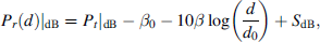
where β₀ is a constant. The term S_dB is a random variable (r.v.), which accounts for random variations of the pathloss. This variable is also known as log-normal shadowing, because it is supposed to be Gaussian distributed with zero mean and variance $σ_{dB}^{2}$ , that is $S_{dB} \sim N (0, σ_{dB}^{2})$ . In this case, the link between any two nodes is a bernoullian random variable with a certain probability p(d). That is, given two nodes, if P_r > γ, where γ is a hardware-dependent threshold, the link can be established. The case of σ = 0, β = 4, d > d₀ is also called the Two-Rays-Ground model and it is a deterministic model.

As said in Section 2.1 D = 4 guarantees a connected network. Thus, it suffices to guarantee a value of Prob(D  2) as close as possible to 1. We have that $P r o b (D \geq 2) = \sum_{2 \leq k \leq 4} (\binom{N}{k}) p (d)^{k} (1 - p (d))^{N - k}$ . For p = 0.95, Prob(D  2) ≍ 0.9995. Thus, based on the grid step d and on (1), we can set the maximum transmission range by solvingp = Prob {P_r(d)|_dB > γ} = 0.95. It is straightforward to show that:

P_{t} (d) |_{dB} = [10 β {log}_{10} d + γ - {erfc}^{- 1} (2 p) \sqrt{(2)} σ] + β_{0},

(2)

where erfc⁻¹ is the inverse of the standard error function. This formula provides the transmission power of each sensor, given a transmission range and a probability or rate of coverage p. This should not be confused with the sensing coverage of the WSN. An obvious effect of shadowing is the random coverage of the transmission range of each sensor. We will have different received powers in different directions. Consequently, the real coverage radius is not constant as in the ideal isotropic radiation case. It is worth noting that although the value in (2) guarantees a connected network, the interference level inside the network could be high, especially in the case of multiple or very close phenomena. The interference in turn directly impacts on the MAC layer and on the average time to set up a connection towards the sink. In our scenario, to simplify these problems, we have one phenomenon only. The radio model parameters are listed in Table 2.

2.4. Cerpa's Model

The previous model might be used in situations where the shadowing phenomenon is relevant, as in urban areas or in areas with moderate density of surrounding objects, like trees, hills, houses, and so on. In other circumstances, a different model could be more appropriate. For example, in open areas where sensors are placed at the ground-level, a Two-Rays-Ground model is enough [8]. It is worth noting that in general the shadowing is not a random process, i.e. given a certain transmission-receiver separation, the path loss is fixed during the communication, although its value is a r.v. A possible case of time-varying shadowing could arise in the case of mobile WSNs, but there are not experimental evidences. However, we will keep this assumption as a matter of comparison.

Table 2
Radio Model and System Parameters

RADIO MODEL PARAMETERS

pathloss coefficient β = 2.7

variance σ²_dB = 16dB

frequency 916MHz

antenna omni

OTHER PARAMETERS

reporting rate T_r = [0.1, 1000]pps¹

interface queue size 50 packets

UDP packet size 100 bytes

detection interval τ 30s

packet per seconds.

Recently, results of measurements taken in real WSNs have shown that the Packet Reception Rate (PRR) between pair of nodes varies with time, and to date there is not a clear explanation of this phenomenon. These measurements are explained in [3]. One of the causes could be the absence of powerful error correcting codes. Powerful error correcting codes are energy hungry and, for a sensor node, they are not energy efficient. Moreover, the PRR rate is correlated with the distance. Links with medium reception rate (40% ∼ 60%) are also asymmetrical, i.e. the PRR changes with respect to the direction of the link. On the other hand, links with low or high PPR are both symmetrical and stable over time. In summary, there is a set of links in the network which are asymmetrical and unstable. We will use these findings in a simplified version, that is by disregarding the correlation and by assuming different PRRs in both directions of every link. This is a worst case analysis. Furthermore, in our simulation studies, the PRR can be reduced also by the contention of the radio medium, which is always present in a decentralized access network. In particular, we will assume that the links PPRs are independent and identically distributed r.vs. The PRR distribution is a uniform r.v. between 0 and PL^max = 0.5. In this model, we call as Cerpa's model, the transmission range is set to d and the transmission power is computed according to the Two-Rays-Ground radio propagation model.

3. Event Detection and Transport

A WSN must face problems which are rarely considered in classical wired and wireless networks. Two factors limit the applicability of standard techniques: the limited computational capacity of the nodes and the scarcity of the radio medium. From the point of view of the application, we are interested in getting as much as possible information about the physical phenomenon the WSN is designed for. In turn, this quantity, say it N*, depends on the characteristics of the physical phenomenon. However, it is clear that the transport of the event data generated by sensors is different from the transport of non-event data, e.g. control packets. For event data, we can tolerate some level of packet loss, as far as the received number of packets, N_r, is greater than N*. This fact is due to the spatial correlation of sensor nodes, that is a high number of sensors can sense the same phenomenon, reporting the same data, or rather spatial-correlated event data. Here, we use the ESRT transport protocol proposed in the model of [2]. In this model, after sensing an event, every sensor node sends UDP-like messages towards the sink node. The sensor node transmits data packets reporting the details of the detected event at a certain transmission rate, T_r. This parameter depends on several factors, as the quantization step of sensors, the type of phenomenon, and the desired level of distortion perceived at the sink node. Note that in the case of discrete events, this scheme is a simple packet repetition scheme. We briefly review the properties of the ESRT protocol. The ESRT approach to the transport of event data has the following assumptions.

The time is divided in detection intervals τ_i, lasting τ seconds.

The system is supposed to be used for event detection. The event is considered to be reliably detected if a certain number of packets N* is received at the sink node. The normalized reliability is defined as η(τ_i) = N_r(τ_i)/N*.

At every event instance, the sink node computes the reliability η(τ_i). Accordingly, the sink node instructs sensor nodes in order to adjust the reporting rate, until the optimal operating point |η − 1| < ∊ is reached. The corresponding transmission rate is called as TO. The optimal operating zone is O = {T_r : |η − 1| < ∊}.

The system is assumed to operate according to the (η, T_r) chart, shown in Fig. 1. This graph divides the plane in 4 operating zones³:

Low reliability and no congestion;

High reliability, low or no congestion (optimal zone);

High reliability, low congestion;

Low reliability, congestion.

The reporting rate, T_r, is changed in a nonlinear fashion. For example, if the system is in the zone I, T_r is subjected to a multiplicative increase. If the system is in the zone IV, T_r is decreased according to an exponential function.

The reliability is computed at every τ_i, thus past information are not taken into account.

The congestion is detected locally by a simple mechanism implemented inside the nodes, which compare successive levels of the buffer of incoming data packets.

Figure 1.

Analysis of stability.

The basic assumption is that a stable operating point exists. This is true in general if N*  max τ_i(N_r(τ_i)), that is we cannot ask sensors to report more packets than those the network can forward (capacity limit). For usual application of WSNs, this is not a problem. The stable point exists if the line η = 1 intercepts the operating curve of the system, as in Fig. 1-a. Otherwise, the system is not stable. For example, in Fig. 1-b, the system is initially unstable (interval τ₁, τ₂), because stable routes towards the sink node are not yet discovered. However, the routing protocol can build a backlist of links not good and exclude them from the path discovery process. This is accomplished in subsequent detection intervals. Eventually, the routing protocol discovers good links and it can build stable paths. The net effect of such irregularities is a prolonged latency in the detection process of the event. This could be a problem in the case of tracking of mobile objects. In Figs. 1-c,d, the system cannot reach a stable point, because the network cannot deliver the required number of packets in the detection interval τ. Let us note that in this case, the routing protocol must discover every time a new set of good links. In the next section, we analyze the factors which could cause the emergence of unstable points or rather situations in which a stable point does not exist.

4. Simulations

In this Section, we present the simulation results of our WSN. We simulated a square lattice sensor network by means of NS-2 simulator, with the support of NRL libraries⁴. Accordingly, we compute η = N_r(τ)/N* as a function of T_r. For every T_r, we fix the detection interval, τ = 30s. In this interval, we count N_r. The value of N* = 700. The number of nodes N is set as power of integers in order to analyse the behaviour of the scaled versions of the network. The initial position of phenomenon node is varied along the simulation runs. The sample averages of η are computed over 20 simulation runs, and they are plotted in Fig. 2, with respect to the particular radio model used. The normalized reliability is a linear function of T_r up to a certain point, T_r ≈ 20 pps, after which the capacity of the WSN limits the maximum number of packets per unit of time which can be injected in. However, for N = 16 we can see a different behavior. The explanation is not simple, because contention losses and congestion losses are intimately related. We can say that at low T_r the contention is low and all source nodes share fairly the radio medium. At a certain value of T_r, the collision rate increases and a number of source nodes are silenced by the MAC backoff mechanism. By increasing T_r a capture effect arises: a fraction of source nodes get control of the channel, while others are silenced in subsequent time slots. Increasing T_r means that also the number of congestion losses increases, as shown in the plot of the goodput, defined as N_r(τ)/N_s(τ). If we consider the Packet Delivery Rate (PDR), by comparing Figs. 3 and 2, we can say that although the number of received packets is greater than N*, the fraction of sent packets which effectively arrived at the sink is very low, especially in the case of the Cerpa's model, as shown in Fig. 3-c. This is due to buffer overflow inside nodes along the path towards the sink node. This approximately explains the irregular trend of η for N = 16. For higher node density, more source nodes try to capture the channel resulting in more MAC collisions, as shown in Fig. 4. This virtually decreases the offered load to the network, with high probability backlogged nodes will find a busy channel as T_r increases.

Figure 2.

Sample averages of the normalized reliability, η.

Figure 3.

Packet delivery rate.

Figure 4.

MAC collisions.

In the case of shadowing, the network has less links and others interfere with distant nodes. The on-demand routing protocols are affected by the presence of shadowing-induced unidirectional links. Even at low T_r, the routing protocol is constrained by the detection interval: We spend more time in finding good paths than transmitting data to the sink node. Let us note that this is the worst case as used by the ns-2 simulator, where at every packet transmission instance a new path loss is computed. Note also that as σ increases, N_r increases with N. This happens because a high value of σ means that we are “adding” other links. However, other phenomena such as the hidden and exposed node problems arise. The situation become worse for the Cerpa's model, where we observe a reduced η for low T_r and high density network (N = 256), and an unpredictable behavior for high values of T_r. We would note here that unstable states pointed out in Section 3 can arise. In other words, given a fixed detection interval, N_r can be much lower than N*, if we take into account links irregularities. This fact might or might not affect the performance of the WSN, because it depends on the requirements of the application, i.e. the value of N*.

As shown in Fig. 5, the average delay towards the sink node increases with T_r. The initial negative slope of the curves for very low values of T_r is due to the fact that the routing protocol has not enough time to discover a stable path and/or all the source nodes are backlogged. For both Shadowing and Cerpa's model the delays increase with respect to the TwoRaysGround case. Note also that in the case of N = 256 in Fig. 5-b, we did not show any data, because the number of samples is not enough to draw any statistical evaluation. In this case, the values of the event-to-sink delay span the entire [0.10]s range. This means that, most of the time, the sink receives packets, and most of the delays are high. Another aspect which affects the PDR is the network interface queue length of nodes which act also as routing nodes, although we did not analyse in this work. Eventually, if all nodes had a constant sensing range, the higher is the node density, the higher will be the number of nodes which can detect the phenomenon and the congestion level inside the network. The most important aspect we would point with these results is that instability states can be present in the system, and this problem strictly depends on the radio environment where the WSN is supposed to operate in.

Figure 5.

Average delay.

5. Conclusions

In this paper, we presented simulation results of a square lattice WSN, with a single sink and fed by a number of sensors nodes which detect a generic physical event. The objective of the paper has been the study of the impact of radio irregularities, for instance the log-normal shadowing and the Cerpa's model, on the performance of a recently proposed transport technique for the event-data. We used the normalized reliability and the PDR as simple metrics to measure the performance. Because of the radio irregularities, we emphasized the fact that the reliability cannot arbitrarily set to high values, regardless of the detection interval τ. In other words, the system has a time factor which depends on the network throughput. By analysing in details the loss process, we found anew the problems of the CSMA based MAC protocols used in a multi-hop context, that is the shadowing is more deleterious at the MAC layer. In contrast to wired networks, the limited and low capacity of the radio medium, the limited computational and memory capabilities of nodes call for new mechanisms of coordination among sensor nodes, e.g. mixed distributed scheduling/contention access schemes. In contrast to most works, we argue that in regard to application algorithms which make use of the underlying propagation model, we cannot afford to neglect the radio irregularities. We are planning to extend the results to other routing and MAC protocols, other non-lattice topologies, and evaluate this framework in real-test bed as well. Nevertheless, although difficult, an analytical approach to the presented results could help understanding and forecasting the behaviour of general networks.

Footnotes

1

By using the theorem in [], we can say that a simple 2-regular network is almost surely strongly 2-connected.

2

Other MAC factors affect the reception process, for example the Carrier Sensing Threshold (CST) and Capture Threshold (CP) of IEEE.802.11 used in ns-2.

3

These figures reproduce the results obtained in [].

4

Since the number of Scheduler events within a simulated WSN can be very high, we applied a patch against the scheduler module of NS-2 in order to speed up the simulation time [].

References

Crossbow technology, inc.

http://www.xbow.com/.

Akan

Özgür B.

and Akyildiz

I. F.

. Event-to-sink reliable transport in wireless sensor networks. IEEE/ACM Transactions on Networking, 13(5):1003–1016, 2005.

Cerpa

Wong

J. L.

Kuang

Potkonjak

, and Estrin

. Statistical model of lossy links in wireless sensor networks. In Proceeding of Fourth International Symposium on Information Processing in Sensor Networks, 2005, pp. 81–88, 2005.

Cooper

. A note on the connectivity of 2-regular digraphs. Random Structures Algorithms, 4:469–472, 1993.

Demirkol

Ersoy

, and Alagöz

. Mac protocols for wireless sensor networks: A survey. IEEE Communications Magazine, 2006.

Donward

. Nrl's sensor network extension to ns-2. http://pf.itd.nrl.navy.mil/nrlsensorsim/, 2004.

Kansal

Ramamoorthy

Srivastava

M. B.

, and Pottie

G. J.

. On sensor network lifetime and data distortion. In Proceedings of International Symposium on Information Theory, pp. 6–10, 2005.

Merrill

W. M.

Liu

H. L. N.

Leong

Sohrabi

, and Pottie

. Quantifying short-range surface-to-surface communications links. IEEE Antennas and Propagation Magazine, 46(3), 2004.

Perkins

, ed. Ad Hoc Networks. Addison-Wesley, 2001.

10.

Rappaport

T. S.

. Wireless Communications. Prentice Hall PTR, 2001.

11.

Tay

Y. C.

Jamieson

, and Balakrishnan

. Collision-minimizing csma and its applications to wireless sensor networks. IEEE Journal on Selected Areas in Communications, 22(6): 1048–1057, August 2004.

12.

Vuran

M. C.

Gungor

V. C.

, and Akan

O. B.

. On the interdependency of congestion and contention in wireless sensor networks. In Proceedings of CST SenMetrics '05, July 2005.

13.

Allen

G.W.

Lorincz

Marcillo

Johnson

, and Ruiz

and Lees

. Deploying a wireless sensor network on an active volcano. IEEE Internet Computing, 10(2):18–25, March 2006.

14.

Wei

D. X.

. Speeding up ns-2 scheduler. http://netlab.caltech.edu/wTeixl/technical/ns2patch, September 2005. California Institute of Technology.

15.

Zhao

and Govindan

. Understanding packet delivery performance in dense wireless sensor networks. In SenSys '03: Proceedings of the 1st international conference on Embedded networked sensor systems, pp. 1–13, New York, NY, USA, 2003. ACM Press.

16.

Zhou

Krishnamurthy

, and Stankovic

J. A.

. Models and solutions for radio irregularity in wireless sensor networks. to appear in ACM Transactions on Sensor Networks, 2006.