Sage Journals: Discover world-class research

Abstract

Multi-hop wireless networks (such as ad-hoc or sensor networks) consist of sets of mobile nodes without the support of a pre-existing fixed infrastructure. For scalability purpose, ad-hoc and sensor networks may both need to be organized into clusters and require efficient protocols to perform common global communication patterns like the broadcasting operation. During a broadcasting task, a source node needs to send the same message to all other nodes in the network. Some desired properties of a scalable broadcasting are energy and bandwidth efficiency, i.e., message retransmissions should be minimized. In this article, we present scalable broadcasting schemes that take advantage of the clustering structure. In this way, we only build one structure to perform both self-organization and broadcasting in clusters and in the entire network. It appears that our broadcasting scheme presents the best trade-off between the number of retransmissions and transmitters (for energy saving) and reliability, when compared to existing solutions.

Keywords

Sensor: Multi-hop Wireless Networks Self-organization Broadcasting Clustering Stochastic Geometry

I. Introduction

Multi-hop wireless networks (such as ad-hoc or sensor networks) consist of sets of mobile wireless nodes without the support of a pre-existing fixed infrastructure. They offer unique benefits for specific environments and applications as they can be quickly deployed. Each node acts as a router and may arbitrary appear or vanish. Protocols deployed in such dynamic contexts must adapt to frequent network topology changes. No centralized administration entity is required to manage the different mobile hosts operations. Mobile hosts rely on battery power, which is a scarce resource. Moreover, wireless links have a significantly lower capacity than wired ones; they may be affected by several error sources that result in a degradation of the received signal. Ad-hoc networks and sensor networks are instances of multi-hop wireless networks. In ad-hoc networks, nodes are independent and may arbitrarily move at any time at different speeds. In sensor networks, nodes are more static and collect data they have to forward to specific sink nodes. For the purpose of scalability, ad-hoc and sensor networks both may need to be organized into clusters and require some protocols to perform common global communication patterns as the broadcasting task. An organization is needed to allow the scalability in terms of number of nodes or/and node density without generating too much traffic (for routing, for example) neither too much information to store or to compute. A common solution is to adopt a hierarchical organization by grouping nodes into “clusters” and bind them to a leader (cluster-head). Such an organization may allow the application of different routing schemes in and between clusters. In a broadcasting task, a source node needs to send the same message to all other nodes in the network. Such a functionality is needed, for example, when some queries about the measures (in sensor networks) or a node location (in ad hoc networks) need to be disseminated over the entire network or within a cluster. Furthermore, in all wireless networks, the broadcasting task is a fundamental mechanism used by either proactive or reactive routing protocols. The desired properties of a scalable broadcasting are thus reachability (every node must be touched by the broadcasting), energy, and bandwidth efficiency (battery power and bandwidth are rare resources and must be saved as much as possible). The operation has to be designed in order to decrease the overhead as much as possible, while maintaining the maximal diffusion.

In this paper, we propose to take advantage of the characteristics of our previous wireless network clustered structure [13] in order to extend it to an efficient and scalable broadcasting structure. By using our purely distributed clustering algorithm, we build only one structure for both operations (organizing and broadcasting). We argue that both emissions and receptions consume energy. In order to maximize the lifetime of the network, one should minimize the number of relay nodes but also the number of receptions induced. We also provide a theoretical analysis of the broadcasting operation in such networks that show that the mean number of receptions per node can be expressed as the product of the degree of relay nodes time the probability for a node to be such a relay. Simulation results then allow us to illustrate our theoretical analysis and to evaluate the reliability of the different broadcasting schemes with regard to the number of the relays and their degree. Surprisingly, it appears that the more reliable protocols are not the ones with the greater number of transmitters but the ones which elect relays with a high degree. They also show that our broadcasting algorithm presents the best trade-off between the number of retransmissions and transmitters (for energy saving) and reliability, when compared to existing solutions.

The remainder of this paper is organized as follows. Section II presents some existing broadcasting solutions. Section III summarizes our previous work and highlights the fundamental characteristics of our cluster organization which might be useful for a broadcasting task. Section IV presents the way we extend our cluster structure into a broadcasting structure and details our broadcasting scheme. Section V provides a theoretical analysis of the broadcasting task using the stochastic geometry and the Palm distribution. Section VI compares several broadcasting schemes by simulation and presents the results. Finally, we conclude and discuss possible future areas of investigation in Section VII.

II. Broadcasting in Multi-hop Wireless Networks

The desired properties of a scalable broadcasting are reachability, energy, and bandwidth efficiency. By reachability, we mean that a great proportion of nodes (more than 90%) receives the broadcast message. In this paper, we only consider reliability at the network layer, i.e., a broadcasting scheme is said to be reliable if every node connected to the source receives a broadcast packet in a collision free environment. As in a wireless environment, a node wastes energy when transmitting as well as receiving a packet [7], the number of retransmissions and receptions should both be minimized. In this section, we focus on solutions proposed in the literature for network layer broadcasting schemes which are based on dominating sets and use omni-directional antennas.

The easiest way to broadcast a message over a network is the blind flooding, i.e., each node re-emits the message upon first reception of it. Obviously, this scheme engenders many collisions and wastes bandwidth and energy. Therefore, this broadcasting technique can not be envisaged over large—scale or very dense networks. This gave birth to more intelligent broadcasting protocols which try to minimize the number of retransmissions by selecting a subset of relay nodes that are allowed to forward a message. This subset is called a dominating set. To obtain a reliable broadcasting scheme, each node in the network should be either in the dominating set (and is called a dominant or internal node) or neighboring at least one node in the dominating set. The main challenge is to find a connected dominating set (i.e., where the dominant nodes form a connected component) which minimizes the number of these transmitters as well as the number of copies of a same message received by a node. However, this problem is known to be NP-hard [9]. I Stojmenovic and J. Wu [19] have classified broadcasting schemes according to the kind of the dominating set they use: cluster-based, source-dependent dominating set, and source-independent dominating set.

In previous cluster-based [6], [11] solutions, the idea is that every node which has the lowest Id or the highest degree (Linked Cluster Architecture (LCA) protocol) in its 1-neighborhood becomes a cluster-head. If a non-cluster-head node can hear more than one cluster-head among its neighbors, it becomes a gateway. The connected dominating set is thus composed of both the cluster-heads and the gateways. Some optimizations have been proposed to localize the maintenance process and avoid chain reactions which may occur in case of node mobility [4] or to limit the number of gateways [22] (to reduce the size of the dominating set).

In solutions based on a source-dependent dominating set [10], [17], the sending node selects adjacent nodes that should relay the message. The set of relays of a node u is chosen to be minimal and such that each 2-hop neighbor of node u has at least one neighbor among the relays of u. A node u only needs information on its 2-neighborhood to select its relays. When a broadcasting task is performed, a node u forwards a message received at first from a node v if and only if node v has chosen node u as one of its relays. Methods differ in details on how a node determines its relays. The most popular of them is the one based on the Multi-Point Relays (MPR) of OLSR [17]. In OLSR, the MPR are also used for building routing tables and the MPR have thus a double use.

In solutions based on source-independent dominating set, the set of relay nodes is independent of the source node and thus it is the case of our proposal. Nodes decide by themselves whether they belong to the dominating set, as opposed to the source-dependent schemes where relays are explicitly chosen by a node. Many solutions have been proposed. In every cases, nodes only need information of their 2-neighborhood. A simple and efficient algorithm, the NES (Neighbor Elimination-Based Scheme) of Wu and Li [21], introduces the notion of intermediate nodes. A node is said to be intermediate if at least two of its neighbors are not direct neighbors. Two selection rules based on the 2-neighborhood topology are then introduced to reduce the number of intermediate nodes by “eliminating” some of them. The remaining ones become the relays. A node states whether it is relay according to a priority value which primarily was the node Id. Then, several variant solutions have been proposed to enhance this algorithm by using other priority values as for e.g. the node degree or the remaining battery [5], [18]. From it, several solutions have then been derived [3], [18]. In [18], the authors also propose another kind of Neighbor Elimination Scheme which can be summed up by “Wait and See”. Upon reception of a broadcast message, a node does not forward the message immediately but counts a random period of time. During this period it watches whether one of its neighbors forwards the message and if so, what are the nodes which receive the message. When the random period is expired, the node forwards the message if and only if some of its neighbors have not been covered by previous transmissions. An enhancement of this scheme has then been introduced in [3] by considering the Relative Neighborhood Graph (RNG) instead of the real graph. However, these latter Neighbor Elimination Schemes can not be classed in source-independent dominating set category as they are based on random numbers. Moreover, the transmitters change from one broadcasting task to another one and do not depend on the source neither. Waith and See protocols obviously obtain great results regarding the number of transmitter nodes and useless receptions but they also induce an important latency due to the random waiting periods.

III. Previous Work and Main Objectives

In this section, we summarize our previous clustering approach on which our broadcasting scheme proposition relies. Only basis and features which are relevant for broadcasting are mentioned here. For more details or other characteristics of our clustering heuristic, please refer to [13], [14], [15]. For the sake of simplicity, let us first introduce some notations. We classically model a multi-hop wireless network, by a graph G = (V,E) where V is the set of mobile nodes (|V| = n) and e = (u,v) ∈ E represents a bidirectional wireless link between a pair of nodes u and v if and only if they are within communication range of each other. We note C(u) the cluster owning the node u and H(u) the cluster-head of this cluster. We note Γ₁(u) the 1-neighborhood of node u, i.e., the set of nodes with which u shares a bidirectional link, δ (u) = |Γ₁(u)| is the degree of u.

Our objectives for introducing our clustering algorithm were motivated by the fact that in a wireless environment, the less information exchanged or stored, the better. First, we wanted a cluster organization suitable for large scale multi-hop networks. That implies that the radius/diameter of clusters should not be fixed a priori but should be flexible radius and able to adapt to the different topologies. (The clustering schemes mentioned in Section II have a radius of 1, in [1], [8] the radius is set a priori.) Second, nodes should be able to set up purely local heuristics by using local information, gathered in their 2-neighborhood. (In [1], if the cluster radius is set to d, the nodes need to gather information up to d hops away before taking any decision.) Finally, we desired an organization robust and stable over node mobility. To satisfy all these requirements, we introduced a new metric called density. The notion of density characterizes the “relative” importance of a node in the network and within its neighborhood. The underlying idea is that this link density (noted ρ(u)) should smooth local changes down in Γ₁(u) by considering the ratio between the number of links and the number of nodes in Γ₁(u).

Definition 1 (density)

The density of a node u ∈ V is

ρ (u) = \frac{| {e = (v, w) \in E ∣ w \in {u} \cup Γ_{1}} |}{δ (u)}

Each node locally computes its density value and periodically broadcasts it locally to its 1-neighbors (e.g., using Hello packets). Each node is thus able to compare its own density value to its 1-neighbors' density and decides by itself whether it joins one of them (the one with the highest density value) or it wins and elects itself as cluster-head. In case of ties, the node with the lowest Id wins. In this way, two neighbors can not be both cluster-heads. By performing the joining process, we actually build directed acyclic graphs (DAG). A DAG is a directed graph that contains no cycles, i.e. a directed tree. The node with the highest density value within its neighborhood becomes the root of the tree and thus the cluster-head of the cluster. If node u has joined node w, we can say that w is node u's parent (noted ρ(u) = w) in the clustering tree and that node u is a child of node w (noted u ∈ Ch(w)). A node's parent can also have joined another node and so on. A cluster then extends itself until it reaches another cluster. If no node has joined a node u (Ch(u) = θ), u becomes a leaf. All the nodes belonging to a same tree belong to the same cluster. The clustering process builds clusters by building a spanning forest of the network in a distributed and local way as the decision criterion is only based on information regarding the 2-neighborhood of a node (gotten from HELLO packets locally and periodically broadcast).

A. Some Characteristics of the Clustering Algorithm

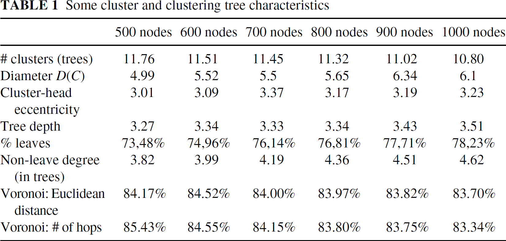
This algorithm stabilizes when every node knows its correct cluster-head value. It has been proved by theory and simulation to self-stabilize within an expected low, constant, and bounded time [15]. It has also been proved that a cluster-head is aware of an information sent by any node of its cluster in a low, constant, and bounded time. The number of clusters built by this heuristic has been showed analytically and by simulation to tend toward a constant asymptote when the density of nodes in the network increases. Moreover, compared to other clustering schemes as DDR [16] or Max-Min d cluster [1], our cluster organization has revealed to be more stable over node mobility and arrivals and to offer better behaviors over non-uniform topologies [13]. Other interesting features for broadcasting obtained by simulations are gathered in Table I. They are commented on in Section III-B.

Table 1
Some cluster and clustering tree characteristics

500 nodes 600 nodes 700 nodes 800 nodes 900 nodes 1000 nodes

# clusters (trees) 11.76 11.51 11.45 11.32 11.02 10.80

Diameter D(C) 4.99 5.52 5.5 5.65 6.34 6.1

Cluster-head eccentricity 3.01 3.09 3.37 3.17 3.19 3.23

Tree depth 3.27 3.34 3.33 3.34 3.43 3.51

% leaves 73,48% 74,96% 76,14% 76,81% 77,71% 78,23%

Non-leave degree (in trees) 3.82 3.99 4.19 4.36 4.51 4.62

Voronoi: Euclidean distance 84.17% 84.52% 84.00% 83.97% 83.82% 83.70%

Voronoi: # of hops 85.43% 84.55% 84.15% 83.80% 83.75% 83.34%

	500 nodes	600 nodes	700 nodes	800 nodes	900 nodes	1000 nodes
# clusters (trees)	11.76	11.51	11.45	11.32	11.02	10.80
Diameter D(C)	4.99	5.52	5.5	5.65	6.34	6.1
Cluster-head eccentricity	3.01	3.09	3.37	3.17	3.19	3.23
Tree depth	3.27	3.34	3.33	3.34	3.43	3.51
% leaves	73,48%	74,96%	76,14%	76,81%	77,71%	78,23%
Non-leave degree (in trees)	3.82	3.99	4.19	4.36	4.51	4.62
Voronoi: Euclidean distance	84.17%	84.52%	84.00%	83.97%	83.82%	83.70%
Voronoi: # of hops	85.43%	84.55%	84.15%	83.80%	83.75%	83.34%

B. Objectives

As explained carlier, our clustering heuristic leads at the same time to the formation of a spanning forest. It appears attractive to use such a “nice” underlying clustering tree structure as a basis for the broadcasting task. This broadcasting scheme is dominating set-based where all non-leaf nodes (tree internal nodes) belong to the dominating set. As mentioned in Table I, a great proportion of nodes (about 75%) are actually leaves, therefore a broadcasting scheme based on this dominating set is expected to save many retransmissions. As the clustering trees form a spanning forest of the network, the set of all trees is a dominating set of the network but is not a connected dominating set as the trees are independent. So, to perform a reliable broadcasting task in the entire network, we need to connect these trees by electing some gateways between them. Our gateway selection process is described in Section IV.

As already mentioned, each node only needs to know its 2-neighborhood to choose its parents, and to know whether it has been chosen as parent by one of its neighbors, otherwise it is a leaf. Thus, the forwarding decision of a non-gateway node is based on local state information.

Only the gateway selection can be qualified as quasilocal (according to the classification of [22]) as only few nodes need information up to 4 hops away (tree depth). Thus, our broadcasting scheme does not induce a high costly maintenance. We propose to use this structure not only to perform a traditional broadcasting in the whole network but also for broadcasting constraint into a cluster only. This kind of task might be interesting for clustered architectures when, for example, a cluster-head needs to spread information only in its cluster like in sensor networks, for instance, where a base station may need to update devices or spread a query over them. The eccentricity of a node is the greater distance in the number of hops between itself and any other node in its cluster. We can see in Table I that the tree depth is pretty low and close to the optimal one (cluster-head eccentricity). This presents a good property for performing a broadcasting within our clusters. Indeed, none of the nodes are really far away from their cluster-head and can expect to receive quickly any information they would spread. Moreover, we computed the proportion of points closer to their cluster-head than any other one in Euclidean distance (Voronoi: Euclidean distance in Table I) and in number of hops (Voronoi: number of hops in Table I). Results show that a large proportion of nodes (more than 83%) lay in the Voronoi cell of their cluster-head, whatever the process intensity. This characteristic is useful in terms of broadcasting efficiency as if the cluster-heads need to spread information over their own cluster, if most of the nodes are closer to the one which sends the information, we save bandwidth, energy, and latency.

IV. Our Contribution

In this section, we first propose an algorithm for the gateway selection, then we detail the two kinds of broadcasting: within a cluster and in the whole network.

A. Gateway Selection

A gateway between two neighboring clusters C(u) and C(v) is a pair of nodes 〈x, y〉 noted gateway(C(u), C(v)) = 〈x, y〉 such that x ∈ C(u), y ∈ C(v) and x ∈ Γ₁(y). For a given pair, we say that node x is the “gateway node” and that node y is the “mirror-gateway node” of the gateway. If C(u) and C(v) are two neighboring clusters, we note the gateway gateway(C(u),C(v)) = 〈x = GW(C(u),C(v)), y = GWm(C(u), C(v))〉, where GW(C(u), C(v)) is the gateway node and GWm(C(u), C(v)) is the mirror-gateway node. Note that GW(C(u), C(v)) ∈ C(u) and GWm(C(u), C(v)) ∈ C(v). The gateways are directed gateways in the meaning that two neighboring clusters are linked by two gateways gateway(C(u), C(v)) and gateway(C(v), C(u)) which may be different.

To select a gateway between two clusters, we thus need to define a pair of nodes. Our selection algorithm runs in two steps. The first step allows each frontier node to locally choose its “mirror(s)” in the neighboring cluster(s). We call a node u a frontier node if at least one of its neighbors does not belong to the same cluster than u. A frontier node and its mirror then form an eligible pair. The second step selects the most appropriate pair as the gateway. The algorithm tries to promote the selection of internal nodes in order to minimize the size of the dominating set as these latter ones already belong to the relay set.

Moreover, in order to add reliability against link failures over these sensitive nodes, each gateway elects a back-up gateway within its neighborhood. This one will forward the message if and only if it does not hear the principal gateway transmitting it (Wait and See philosophy).

1) Mirror node selection

As seen in Section III, as the density-based clustering algorithm uses the node Id as the last decision criterion, every node u might be aware in an expected bounded and low time, whether there exists among its neighbors a node v which does not belong to the same cluster than u. If so, node u is a frontier node and so becomes an eligible gateway node for Gateway(C(u), C(v)). Each frontier node u then selects its mirror node among its neighbors which do not belong to C(u). To do so, u first selects non-leaf nodes, i.e., internal nodes/transmitters in every case and choses among them the node with the highest density value. If all nodes r ∈ Γ₁(u) such that C(u) ≠ C(v) are leaves, u chooses the node with the lowest degree in order to limit the useless receptions induced by an emission of a message by the mirror. In case of ties, the lowest Id decides. If u is a frontier node of the cluster C(v) (C(v) ≠ C(u)), we note m(u,C(v)) the mirror node chosen by u in C(v). Note that if a node u is a frontier node for several clusters, it has to select a mirror for each cluster.

Algorithm 1

Mirror selection - RUN AT EACH FRONTIER NODE u, i.e., ∃v ∈ Γ₁(u) s.t. C(v) ≠ C(u)

2) Gateway selection

Once each frontier node has chosen its mirror, we have to choose the most appropriate pair as the gateway. Once a gateway node u is elected as GW(C(u).C(x)), we have Gateway(C(u), C(v)) = 〈GW(C(u).C(x)).mirror(GW(C(u), C(x)), C(x))〉. According to the taxonomy of [22], this step is quasi-local whereas the first one is local.

The gateway selection we propose is distributed since a selection is performed at every level in the tree and tries to limit useless receptions by favoring internal nodes. Frontier nodes send their Id to their parent and indicate them whether they are leaves and whether they have a leaf as mirror. Each parent selects the best candidate among its children and sends the same information up to its own parent and so on, until reaching the cluster-head. The selection is thus semi-distributed as every internal node eliminates some candidates. In this way, only small size packets are forwarded from the frontier nodes to the cluster-head. As mentioned in Table I, the mean degree of all the internal nodes (cluster-head included) is small and constant whatever the number of nodes, which induces a small and bounded number of messages at each level which is also bounded by a low constant [15].

Let us express that v belongs to the subtree rooted in u (noted v ∈ sT(u)) if u is the parent of node v or if the parent of node v is in the subtree rooted in u:

{v \in s T (u) \cap Γ_{1} (u)} \Leftrightarrow {v \in C h (u)} or {v \in s T (u) \cap Γ_{1} (u)} \Leftrightarrow {P (v) \in s T (u)}

Let us say that C(x) is a neighboring cluster of the subtree sT(u) of an internal u iff C(x) ≠ C(u) and ∃x ∈ C(x) and y ∈ sT(u) such that y ∈ r₁(x). The best candidate choice is performed as follows. For each of the neighboring clusters C(x) of its subtree, an internal node u considers the set G of the candidate nodes (frontier nodes) (G = {v ∈ sT (u) | ∃w ∈ Γ₁ (v) | C(w) ≠ C(u)}). Then, it selects among them the subset G' ⊂ G of internal nodes, still in order to limit the number of transmitter nodes. If G' is only composed of leaves, the selection is processed among all candidates of G. From there, u favors the nodes which mirror is a non-leaf node, then it uses either the density value (if remaining candidates are non-leaves) or degree (otherwise) to decide. At the end, in case of ties, the node with the lowest Id is elected as GW(C(u), C(x)). Note that, if C(u) and C(v) are two neighboring clusters, Gateway(C(u), C(v)) ≠ Gateway(C(v), C(u)) in most cases.

Algorithm 2

Gateway selection RUN AT EACH INTERNAL NODE u

3) Back-up gateway selection

This selection is a purely distributed local process and it derives benefits from the locally broadcast feature offered by the wireless medium. When a frontier node sends information to its parents during the gateway selection process, every node in its neighborhood learns its condition (leaf, internal, border node, etc.). In this way, a gateway node knows in its neighborhood which node may act as a back-up gateway, without extra-message. It selects it by choosing a frontier node which has a mirror node different from its own one if possible. This back-up gateway acts as follows. Upon reception of a broadcast message, the back-up gateway triggers a timeout. If it has not heard the main gateway emitting when the timeout expires, the back-up gateway forwards the broadcast message. This back-up gateway thus does not add any useless receptions (as it emits only under some conditions) and adds some reliability in the broadcasting task. Moreover, it does not add any extra-cost since its selection is local and does not need any additional information.

This back-up gateway concept is similar to the one in “OSPF”¹ where there are back-up routers.

B. Broadcasting Heuristic

A node u may need three kinds of broadcasting tasks:

link-local broadcasting: broadcast to the 1-neighbors of u, no forwarding needed

site-local broadcasting: broadcast to every node in the same cluster than u

global broadcasting: broadcast to all the nodes in the network

To distinguish between these three broadcasting tasks, we need the use of several broadcasting addresses in the packet.² When the broadcasting task is performed within a cluster C(u), the message is forwarded upon first reception by all the non-leaf nodes of C(u). When the broadcasting task is performed in the entire network, all the non-leaf nodes in the network forward the message as well as all gateways and mirror-gateway nodes, under some conditions. As our gateways are directed, a gateway node GW(C(u). C(w)) forwards the message only if it is coming from its own cluster C(u). A mirror-gateway node GWm(C(u), C(w)) forwards the message only if it is coming from the cluster C(u) for which it is a mirror. However, a mirror-gateway node GWm(C(u), C(w)) forwards a message coming from C(u) whatever the transmitter node in C(w) (which is not necessarily the gateway node GW(C(u). C(w)) for which it is the mirror).

Algorithm 3

Broadcasting algorithm

V. Theoretical Broadcasting Analysis

As we saw in Section II, most of the broadcasting protocols aim to reduce the number of transmitters, often by electing the highest degree nodes. The main goal is to minimize the global energy spent for transmission in the network during a broadcasting task. However, as studied in [7], energy spent in receptions is not negligible since a wireless node spends almost the same amount of energy for receiving than for transmitting with the IEEE 802.11 MAC layer technology.

Therefore, in this section, we are interested in the analysis of the number of messages received by a typical node when a broadcasting task is performed.

We will consider that nodes are distributed in the plan according to a stationary Point Process of intensity λ that represents the nodes. In such processes, the intensity λ corresponds to the mean number of points per surface unit. Two points (x,y) of the Point Process are neighbors if and only if the Euclidean distance between x and y is lower than a fixed threshold, a given constant R (d(x,y) ≤ R). R denotes the radio range of the nodes. If Φ is a stationary Point Process of intensity λ, then Φ(S) represents the number of points of the Point Process Φ laying in the surface S. Let B(x, R) be the ball of radius R centered in node x and B′_x be such that B′_x = B(x, R)\{x}.

In Propositions 1 and 2, we express the mean number of receptions per node. This result will be used to compare the different algorithms. Proposition 1 holds for the model we consider in our simulations, which is described in Section VI.

The hypothesis of these propositions are thus directly checked with the model used in this paper. The second result expressed in Proposition 2 is the same than the first one but holds for more general random graphs. Let r̅ be the mean number of receptions received at a node (relay or not). For the sack of clarity, the proofs are presented in Appendix.

Proposition 1

Let Φ be a stationary Point Process of intensity λ (λ > 0) distributed in the plan. Let Φ _Relay be a thinning of Φ. The points of Φ _Relay represent the relays. We suppose that Φ _Relay is still a stationary Point Process of intensity λ _Relay . We only consider nodes/points within an observation window W, which is a square of size L × L with L × R. We have:
$\bar{r} = E_{Φ}^{o} [Φ_{R e l a y} (B_{0}^{'})] = E_{Φ_{R e l a y}}^{o} [Φ (B_{0}^{'})] P_{Φ}^{0} (0 \in Φ_{R e l a y}) = \frac{λ_{R e l a y}}{λ} E_{Φ_{R e l a y}}^{0} [Φ (B_{0}^{'})]$
(1)

where $E_{Φ}^{o} [Φ_{R e l a y} (B_{0}^{'})]$ is the expectation (so the mean number) under palm probabilities w.r.t. the process Φ of the relay points in B′₀.

This latter result may be interpreted as follows: the mean number of receptions per node is the product of the degree of a relay and of the probability for a node to be a relay (or equivalently the mean ratio of relays/nodes).

Proposition 2

Given a random graph G(V, E) and a set of relay nodes Relay ⊂ V, where
(i) the degree of the nodes are identically distributed,

(ii) the degree of the relays in G are identically distributed,

(iii) the number of receptions per node are identically distributed.

Then we have:
$\bar{r} = E [δ (v_{1})] | v_{1} \in R e l a y | P (v_{1} \in R e l a y)$
(2)

In this equality, v₁ is a node arbitrarily chosen among the set of vertice in G (a typical node). The choice of v₁ has no impact since the probability to be a relay and the degree of nodes are equi-distributed. As in Proposition 1, the mean number of receptions per node is the product of the mean degree of the relays and the probability for a node to be a relay.

Discussion

In [7], the authors show that the energy consumption of a broadcast transmission when using the IEEE 802.11 MAC layer technology, is approximately four times the cost of a reception by a node.

In all broadcasting heuristics mentioned in Section II, between 20% and 50% of the nodes are transmitters but each node receives the broadcast message between 5 and 10 times. Therefore, for a 100-node network, a broadcasting operation causes between 20 and 50 transmissions but also between 500 and 1000 receptions. The most expensive part of a broadcasting in a 802.11 ad hoc network is then due to the induced receptions rather than to the transmissions. This key observation may differ from one technology to another, but receptions still certainly consume an important part of the energy spent during a broadcasting. Moreover, a high number of receptions per node increases the collision probability and the bandwidth used. A node which receives 10 times the same packet cannot use the medium during these 10 transmissions. So, we are convinced that one of the main performance criteria for a protocol/heuristic used to broadcast a packet in an ad hoc network is the mean number of receptions per node.

In this Section, we have shown that this number of receptions is given as the product of the proportion of transmitters and the mean degree of the transmitters. Unfortunately, neither the degree of relays nor the proportion of relays can be analytically worked out yet for the considered algorithms but the blind flooding, for which the results are trivial. However, we evaluate these quantities by simulation in Section VI in order to compare the behavior of the different broadcasting algorithms. We shall show that they minimize either the degree of the relays (as the MPR or NES heuristic) or the number of relays used (as our clustering algorithm). For instance, our heuristic based on the node density favors relays with high degree compared to the other heuristics while keeping a low number of receptions (the number of transmitters is then small). It has the advantage of minimizing both transmissions and receptions and hence the global cost of the broadcasting. Moreover, such a relay selection is robust since a transmitter has a high degree: a link failure does not isolate the transmitters.
VI. Simulation Results

We first performed simulations in order to qualify the gateways elected and then to compare the broadcasting tasks performed with our clustering and gateway selection schemes to other existing heuristics. This section details the results. All the simulations follow the same model. We use a simulator we developed which assumes an ideal MAC layer. Nodes are randomly deployed using a Poisson Point Process in a (1 + 2R) × (1 + 2R) square with various levels of intensity λ. In such processes, λ represents the mean number of nodes per surface unit. Only the points within the square w of size 1 × 1 are taken into account to estimate the different quantities (mean degree, mean density, etc.). But in order to avoid side effects, the samples of Point Processes are generated in a larger window W. For instance, if we estimate the mean degree ( $\bar{δ}$ ) of nodes, we take the degree of the points in w to compute $\bar{δ}$ . If we do not consider the points of W, the points close to the edge within w would have a lower degree than the points close to the center, introducing a bias in the estimations. Both windows are shown in Fig. 1. This technique is called “minus-sampling,” a more detailed description can be found in [20]. The communication range R is set to 0.1 in all tests. In each case, each statistic is the average over 1000 simulations. When several algorithms are compared, they are compared with the same samples of the simulation model.

Figure 1

Only points of w are taken into account to estimate the different quantities, but the Point Process is generated in the square W in order to avoid the side effects.

A. Gateways: Election and Utilization

If we consider two neighboring clusters C(u) and C(v), we may have four different types of gateways between them:

Leaf↔Leaf gateways: GW(C(u), C(v)) and GWm(C(u), C(v)) are both leaves. This kind of gateway is the more costly as it adds two transmitter nodes and thus induces more receptions.

Leaf↔Internal Node gateways: GW(C(u), C(v)) is a leaf and GWm(C(u), C(v)) an internal node. This kind of gateway adds only one transmitter node. It is the least popular, as shown later by simulations.

Internal Node↔Leaf gateways: GW(C(u), C(v)) is an internal node and GWm(C(u), C(v)) a leaf. This kind of gateway adds only one transmitter node.

Internal Node↔Internal Node gateways: GW(C(u), C(v)) and GWm(C(u), C(v)) are both internal nodes. This kind of gateway is the one we try to favor since it does not add any extra-cost since it does not add any transmitter neither induces any additional reception. But as we will see, they unfortunately are the least popular ones.

Table 2 shows the mean number of gateways a cluster has to elect and maintain and the mean number of gateways used when a global broadcasting task is performed. As we can note, the number of gateways to elect is reasonable and remains almost constant while the process intensity increases. This shows the good scalability feature of this heuristic. Nevertheless, this was predictable since, as we saw in Section III, the number of clusters is constant from a certain amount of nodes, so is the mean number of neighboring clusters for a cluster and so the number of gateways to elect. Moreover, we also saw that the cluster topology was close to a Voronoi tessellation. Yet, in a Voronoi tesscllation, a cell has 6 neighbors on average. This is actually the mean number of gateways a cluster has to elect. Figure 2(a) gives the proportion of each kind of gateways selected. We can note that the two less elected kinds of gateways are the Leaf↔Internal Node and Internal Node↔Internal Node gateways. This is due to the fact that, by construction, most of the frontier nodes are leaves. This also explains the great proportion of other kinds of gateways since, as soon as there is an internal node as a frontier node, it is elected (and thus Internal Node↔Leaf gateways are preferred to Leaf” Internal Node ones). The more sparse the network, the less chance to find internal nodes on borders. So, the proportion of Internal node↔Leaf gateways increases with the intensity process while the proportion of Leaf↔Leaf gateways decreases.

Figure 2

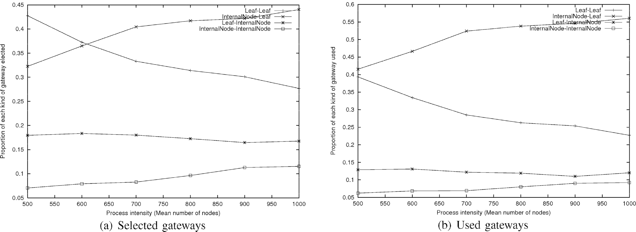
Proportion of each kind of selected gateways and used gateways per cluster as a function of the process intensity (+: Leaf↔Leaf: ×: Internal Node↔Leaf; *: Leaf↔Internal Node; □: Internal Node↔Internal Node)

When a global broadcasting task is performed, all the gateways are not necessarily used since 2 neighboring clusters C(u) and C(v) are connected via 2 gateways Gateway(C(u), C(v) and Gateway(C(v), C(u)) and in most cases, only one of them is used. As shown in Table 2, the number of gateways used per cluster is quite constant and remains pretty low, always comprised between 1 and 2. This means that generally, either the broadcasting enters a cluster and dies in it (in this case, it uses only one gateway), or it passes through it and thus uses two gateways (one to enter the cluster and one to leave it).

Table 2

Number of Gateways Selected and Used per Cluster for a Global Broadcasting Initiated at a Randomly-chosen Source as a Function of the Process Intensity

	500nodes	600nodes	700nodes	800nodes	900nodes	1000nodes
#clusters	11.93	11.64	11.36	11.30	11.14	10.72
#gw selected per cluster	5.86	6.02	6.16	6.20	6.22	6.26
#gw used per cluster	1.76	1.74	1.73	1.76	1.68	1.66

Figure 2(b) shows the proportion of each kind of gateways used when a global broadcasting operation is initiated. As we can see, most of them are the ones which add only one transmitter node. This is true even for low intensities of node when the rate of Leaf↔Leaf gateways elected was the highest. This shows that our algorithm can adapt and favor internal nodes naturally. As the mean number of gateways used is low and since we add only one transmitter node for each gateway, the induced cost is low as well.

B. Broadcasting Performances

In order to evaluate our algorithm, we chose to compare it to some of the most representative broadcasting schemes seen in Section II: blind flooding, LCA [11] (cluster-based schemes). Multi-Point Relay [17] (source-dependent dominating set), the Neighbor Elimination-Based Scheme of Wu and Li [21] (source-independent dominating set), and the Neighbor Elimination Scheme “Wait and See” of I. Stojmenovic, M. Seddigh, and J. Zunic [18] (random dominating set). As seen in Section V, we try to compare them in terms of energy-efficiency, also taking into account the impact of the relay degree on these performances. Therefore, the significant characteristics we note are the proportion of nodes which need to re-emit the message (size of the dominating set) and their mean degree, as well as their impact over the mean number of copies of the broadcast message that a node receives (useless receptions). Moreover, we simulate two different variants of the Neighbor Elimination Scheme of Wu and Li: the original one [21] where the node priority is the node Id, and a later version of it where the priority value is the node degree (plus Id to break ties) [5], still in the aim to study the impact of the relay degree over the broadcasting performances. We also have a look at the latency (time needed for the last node to receive the broadcast packet initiated at the source). As the main goal is to limit energy consumption and bandwidth occupation in order to maximize the network lifetime, all these values have to be as low as possible. Moreover, we have to note that the latency of the NES-“Wait and See” protocol depends on the size of the window in which nodes randomly choose their backoff time. It is thus the protocol with the highest latency and we did not evaluate it.

The more transmitters and useless receptions, the more the redundancy. Thus, when a broadcasting scheme induces many retransmissions, it is expensive in terms of energy but it is expected to be more reliable against link or node failures and/or mobility. Therefore, we also analyze the impact of both number of receptions per node and degree of the relays on the broadcasting robustness. In other words, we analyze the trade-off between redundancy and reliability against link failures.

1) Broadcasting over the whole network (global broadcasting)

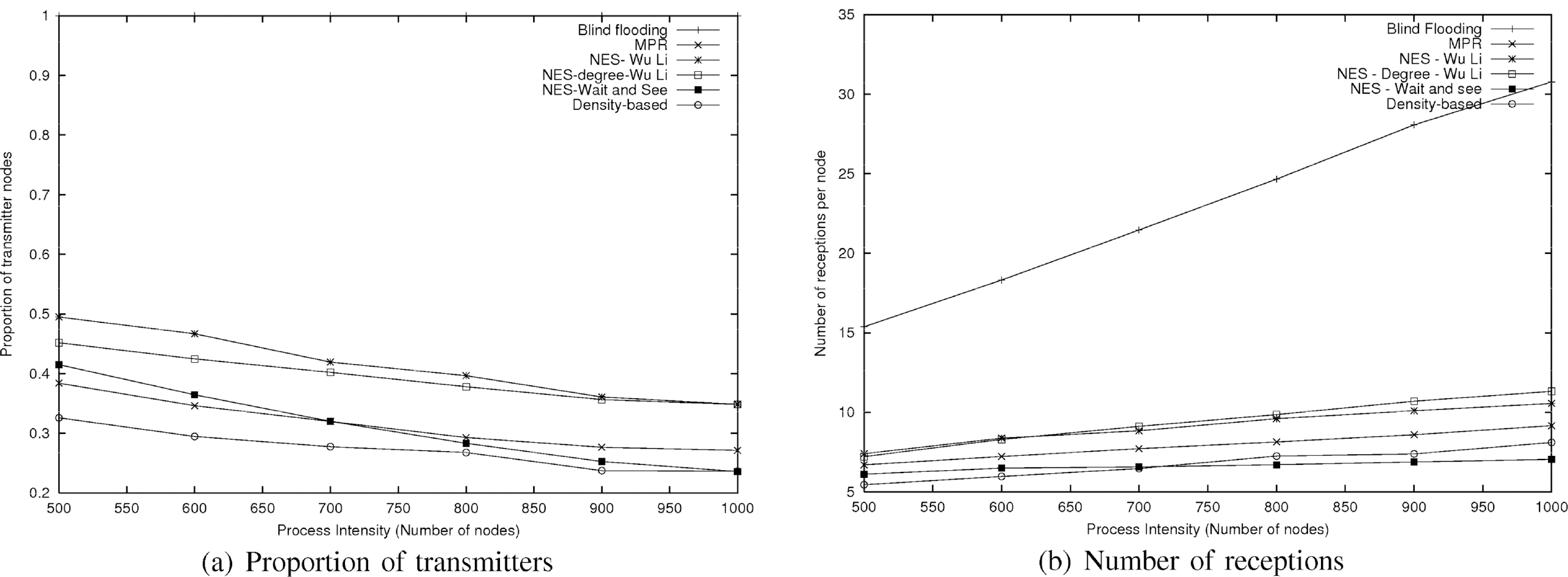
Figure 3 shows the proportion of transmitters in the network as well as their degree in the graph, for the different broadcasting algorithms.

Figure 3

Proportion of transmitter nodes (a) and their mean degree (b) as a function of the mean number of nodes for different algorithms (+: Blind Flooding; ×: LCA; *: MPR; □: NES − Wu Li; ■: NES − Degree − Wu Li; ○: NES − Wait and See; ●: Density-based).

Figure 3(b) shows the degree of these relays. As in the blind flooding, every node is a transmitter, the mean degree of the relays actually is the mean degree of the nodes in the graph. We observe that the density-based relay selection maximizes the mean degree of the relays as opposed to the NES technique of Wu and Li for which the mean degree of transmitters is smaller than the mean degree of nodes. Since the mean node density value is almost proportional to the mean node degree [12], density-based selection elects nodes with a high degree. Besides, note that the original NES of Wu and Li and the NES-“Wait and See” elects transmitters with the same degree value. We also note that the MPR selection elects transmitters without favoring nodes with small or high degree. NES-“Wait and See” selects relays with a degree lower than the mean value as the more neighbors a node has, the more likely it is to hear one of them emitting before its backoff time is off. Moreover, as expected, since heuristics are based on it. LCA and NES-degree of Wu and Li also elect relays with a high degree.

Figure 3(a) plots the proportion of transmitter nodes in the network. As in blind flooding, every node forwards the message upon its first reception and this proportion is equal to 1. We can note that the “Wait and See” heuristic is the one having fewer transmitter nodes and thus spending less energy for emissions. Our heuristic is very close to it. Also note that the two variants of the NES protocol generate approximatively the same amount of transmitters.

Nevertheless, as seen in Section V, the resulting number of receptions per node could not have been deduced only from these results (proportion of transmitters and their degree) as it actually is the convolution of both of them. And, as one of the heuristics with the lowest number of transmitters also is the one with the highest relay degrees, we can not deduce from it whether useless receptions are minimized or not, and so it is for all heuristics. We can just suppose that the variant of the NES protocol based on the degree would cause more receptions on nodes than the original NES protocol as, for a same amount of transmitters, the degree of relays is higher.

Figure 4 shows the mean number of receptions per node of a single broadcast message.

Figure 4

Number of receptions per node as a function of the number of nodes for different algorithms. (+: Blind Flooding; ×: LCA; *: MPR; □: NES − Wu Li; ■: NES–Degree Wu Li; ○: NES − Wait and See; ●: Density-based).

As we can observe, when a global broadcasting task is initiated, the NES-“Wait and See” algorithm induces less receptions than other algorithms. Thus, it spends less energy and resources. Nevertheless, we can note that the results of our algorithm are very close to the “Wait and See” ones since the density-based generates only one additional reception in average per node. Moreover, as the “Wait and See” scheme is based on random counters, the latency induced is inevitably greater than the one induced by the density-based heuristic. Thus, also regarding the fact that the initial goal of density-based heuristic is clustering, we can estimate that the density-based algorithm results are pretty good. Moreover, as mentioned later, the NES-“Wait and See” scheme is much less reliable against link failures. Also note that, as expected, the original NES protocol of Wu and Li creates fewer receptions than the variant based on the node degree.

Since in the MPR selection, the relays are selected in order to reach the 2-neighborhood after two hops, the k-neighborhood of the source is reached within k hops. Under the assumption of an ideal MAC layer, MPR gives the optimal results in terms of latency (Number of hops). We thus compare our heuristic to the MPR one to measure how far we are from the optimal solution. We consider a time unit as a transmission step (i.e., 1 hop). Table 3 presents the results. Yet, we can note that, even if our algorithm is not optimal regarding the latency, results are very close to it. Figure 5 represents the propagation in time for a broadcast packet initiated at the centered source at time 0. Cluster-heads appear in blue and the source in green. The color of other nodes depends on the time they receive the broadcast packet. The darker the color, the shorter the time.

Figure 5

Propagation time of a general broadcasting initiated at a centered source (a) using MPR and (b) using density-based clustering trees.

Table 3

Mean and Max Time for Receiving the Message. “MAX” values represent the time needed for the last node to receive the packet. “MEAN” values represent the mean time a node needs to receive the broadcast packet.

	500 nodes		700 nodes		800 nodes		900 nodes		1000 nodes
	MEAN	MAX	MEAN	MAX	MEAN	MAX	MEAN	MAX	MEAN	MAX
MPR	5.13	8.97	4.88	8.40	4.88	8.40	4.81	8.23	4.78	8.07
Density	6.31	11.05	6.22	10.78	6.24	10.95	6.15	10.66	6.19	10.74

2) Broadcasting within clusters (cluster broadcasting)

We now suppose that the broadcasting task is performed in each cluster, initiated at the cluster-heads. We thus have as many broadcastings as clusters.

We can see in Fig. 6, that this time, our broadcasting algorithm is the one which best minimizes the proportion of transmitter nodes, even outperforming the NES “Wait and See” protocol (Fig. 6(b)). Moreover, it also obtains the best results regarding the number of receptions (Fig. 6(a)) with the NES “Wait and See” Scheme.

Figure 6

Mean number of receptions per node (a) and Proportion of transmitter nodes (b) for a cluster broadcasting scheme w.r.t. the process intensity and the metric used (+: Blind Flooding; ×: MPR; *: NES − Wu Li; □: NES − Degree Wu Li; ■: NES − Wait and See; ●: Density-based).

These results also confirm the analytical results claiming that the number of receptions on nodes can not be directly deduced from the proportion of transmitters. Indeed, for example, the density-based algorithm selects less relays with much higher degree than the “Wait and See” and finally, they both provide a similar amount of receptions per node.

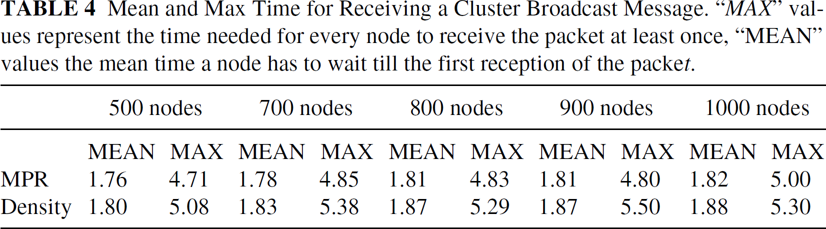
Table 4 and Fig. 7 present the results regarding the latency. We still compare our algorithm to the MPR protocol, without considering the “Wait and See” for which the latency is random as linked to the size of the backoff counter. Once again, we can observe that, even if our algorithm is not optimal, results are very close as, in average, a node our algorithm needs only 0.5 step more than the optimal value to receive the packet. This also shows that, even if routes in trees, from the cluster-heads to other nodes, are not always the shortest ones, they are very close to them.

Figure 7

Propagation time of a cluster broadcast packet over the topology plotted in (a) using MPR (b) or density-based trees (c).

Table 4

Mean and Max Time for Receiving a Cluster Broadcast Message. “MAX” values represent the time needed for every node to receive the packet at least once, “MEAN” values the mean time a node has to wait till the first reception of the packet.

	500 nodes		700 nodes		800 nodes		900 nodes		1000 nodes
	MEAN	MAX	MEAN	MAX	MEAN	MAX	MEAN	MAX	MEAN	MAX
MPR	1.76	4.71	1.78	4.85	1.81	4.83	1.81	4.80	1.82	5.00
Density	1.80	5.08	1.83	5.38	1.87	5.29	1.87	5.50	1.88	5.30

In Table 5, we give the proportion of nodes which receive the first copy of the packet by their parent or by one of their children. This feature shows whether the message which is sent by the cluster-head follows the branches of the trees. Indeed, a node u always receives the message by its parent (as all non-leaf nodes forward the message) but it could have received it before from another path as paths are not always optimal. In this case, as we suppose an ideal MAC layer, the shortest route between u and its cluster-head is not found by following the route in the tree. We can thus see that routes are the shortest ones in number of hops for more than 70% of the cases. We can also observe, as the message progresses down the tree, that none of the nodes receives it first from one of their children.

Table 5

Proportion of nodes which receive the first copy of the packet by their parent or by one of their children

	500nodes	600nodes	700nodes	800nodes	900nodes	1000nodes
% by parent	78.74%	76.81%	74.57%	73.21%	71.31%	70.13%
% by a child	0.00%	0.00%	0.00%	0.00%	0.00%	0.00%

C. Broadcasting and Gateway Reliability

After considering these results, we wonder about the reliability of all these protocols (still only considering the network layer) against link and/or node failures. Indeed, till now, we have only compared protocols regarding the energy saved by each of them, by limiting useless receptions on nodes and trying to minimize the size of the dominating set. However, the more the transmitters, the more the redundancy and thus the more the reliability. Therefore, is it really a good approach to minimize redundancy on nodes in an environment where wireless links are weak? Moreover, we wonder whether the degree of relay nodes has any impact over the reliability. For the same amount of receptions on nodes, is it better to have few transmitters with high degrees or more transmitters with low degrees? And, does the redundancy in terms of number of receptions really has an impact on reliability?

In order to evaluate this aspect of the broadcasting task, we apply a failure probability over links and measure the proportion of nodes still receiving the broadcast message. The simulation tests we performed, assume that the broadcasting task occurs before the nodes have recomputed anything e.g., their set of MPR-Selector nodes (MPR heuristic), their set of neighbors to climinate (every NES scheme) or their parent in the clustering tree (density-based algorithm). As in the blind flooding, every node transmits the message upon first reception of it, nodes do not receive the message only if the network is disconnected. This failure model may seem not to be very realistic as links can also fail because of congestion. Since the blind flooding, for example, induces more messages than any other protocol, more links fail. Nevertheless, the results of the blind flooding give an information about the network connectivity. However, link failures may also be due to node mobility. These moves are not instantly taken into account by the protocols and thus may introduce unexpected behaviors during a broadcasting operation.

Figure 8 shows the results for both kinds of broadcastings: in a cluster and in the whole network, for λ = 1000. Globally, the behavior of different heuristics is the same from one kind of broadcasting task to the other one, except the density-based heuristic. For example, the NES- “Wait and See” which was the best heuristic regarding the number of useless receptions and transmitters, is the least reliable one, whatever the kind of broadcasting.

Figure 8

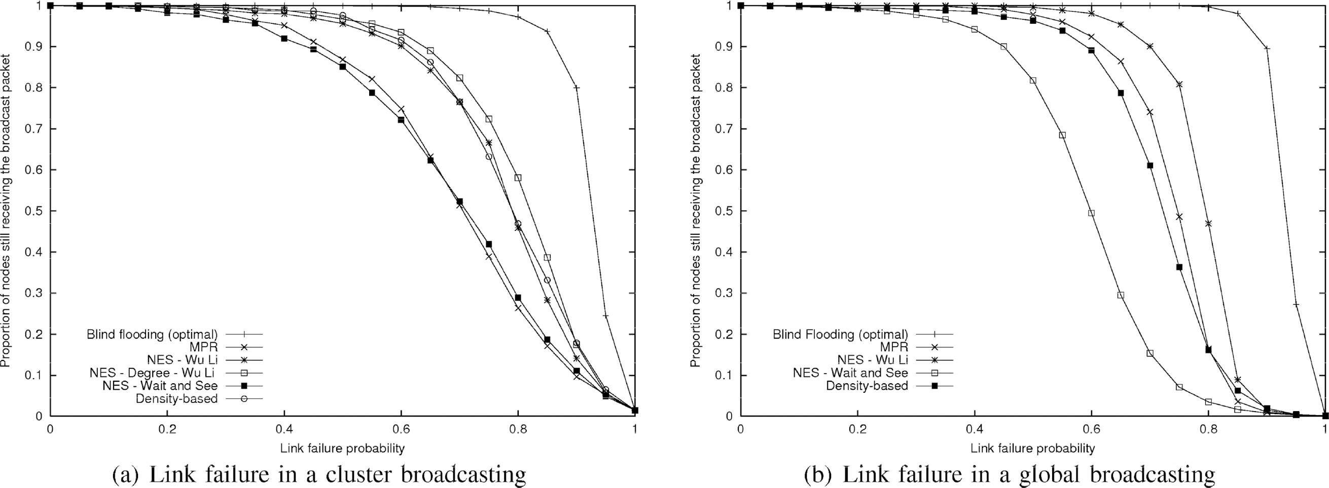
Proportion of nodes still receiving a broadcast message when applying a link failure probability (a) for a cluster broadcasting and (b) for a global broadcasting scheme.

Figure 8(a) considers a broadcasting in a cluster. Surprisingly, it does not appear that there is a link between the mean number of receptions per node, which can be seen as a kind of redundancy, and the robustness. For instance, we can note that even if the MPR heuristic induces more transmitters and useless receptions than that of the NES algorithms of Wu and Li, it is less reliable. This is due to the fact that in the MPR algorithm, a node will forward a broadcast message if and only if it has received the first from a node which has elected it as an MPR [2]. Another example is the density-based heuristic where the number of receptions per node is small but which is one of the most robust.

It seems that protocols, where the relays have a high degree, tend to be more robust. Indeed, heuristics with high degree (NES-degree and Density based) are very robust and protocols with small degrees as MPR or the NES- “Wait and See” present the worst behavior. However, the NES-Wu Li algorithm is an exception but its variant NES-degree (which increases the degree of the relays) is better in terms of robustness. The redundancy in terms of number of receptions is thus very costly in terms of used bandwidth and energy consumption, as discussed in the previous sections, but does not offer better performances in term of robustness.

Therefore, the density-based heuristic presents a good reliability against link failures when a broadcasting task is performed within a cluster. As it also minimizes both the proportion of transmitters and useless receptions on nodes, it constitutes the most efficient protocol since it is a trade-off between cost and reliability. Moreover, it is a reminder that a broadcasting operation in a cluster is performed in a quasi-optimal time.

Nevertheless, as we can notice in Figure 8(b), the density-based algorithm is much less reliable when used for performing a broadcasting task over the entire network. It is still better than the NES- “Wait and See” heuristic as a greater proportion of nodes still receives the message when links fail, but it is less reliable than the NES scheme of Wu and Li. This result, coupled with the fact that our heuristic behaves well when the broadcasting is confined in a cluster, shows that the weakest points in such a global broadcasting are the gateways which link the clusters. Indeed, if a cluster A can be reached only by cluster B and that the gateway from B to A fails, the whole cluster is isolated in the broadcasting operation. In order to add some reliability, it ought to be better to elect several gateways between all pairs of neighboring clusters. Electing more than one gateway does not add extra-cost as the gateway selection manages it without any additional message. Additional cost when using several gateways only appears when a global broadcasting task is performed and uses these multiple gateways. Indeed, this translates to additional transmitter nodes and thus additional receptions on nodes. Therefore, there is a trade-off to discuss between the cost of additional transmitters and useless receptions and the reliability of the protocol. In order to estimate this trade-off, we simulated a global broadcasting by using several gateways between clusters. We then compare with other heuristics regarding the redundancy, the transmitter ratio and the number of useless receptions. Results, given in Fig. 9, clearly show that reliability is quickly improved with the addition of gateways, which confirm that they indeed are the sensitive points in the broadcasting task. As Fig. 9(a) shows, electing three gateways between any pair of neighboring clusters is enough to obtain the same reliability than the NES schemes of Wu and Li. Moreover, as Figs. 9(b) and 9(c) plot, with three gateways, the density-based algorithm still induces less useless receptions and transmitters than other ones (excepted the NES “Wait and See” scheme).

Figure 9

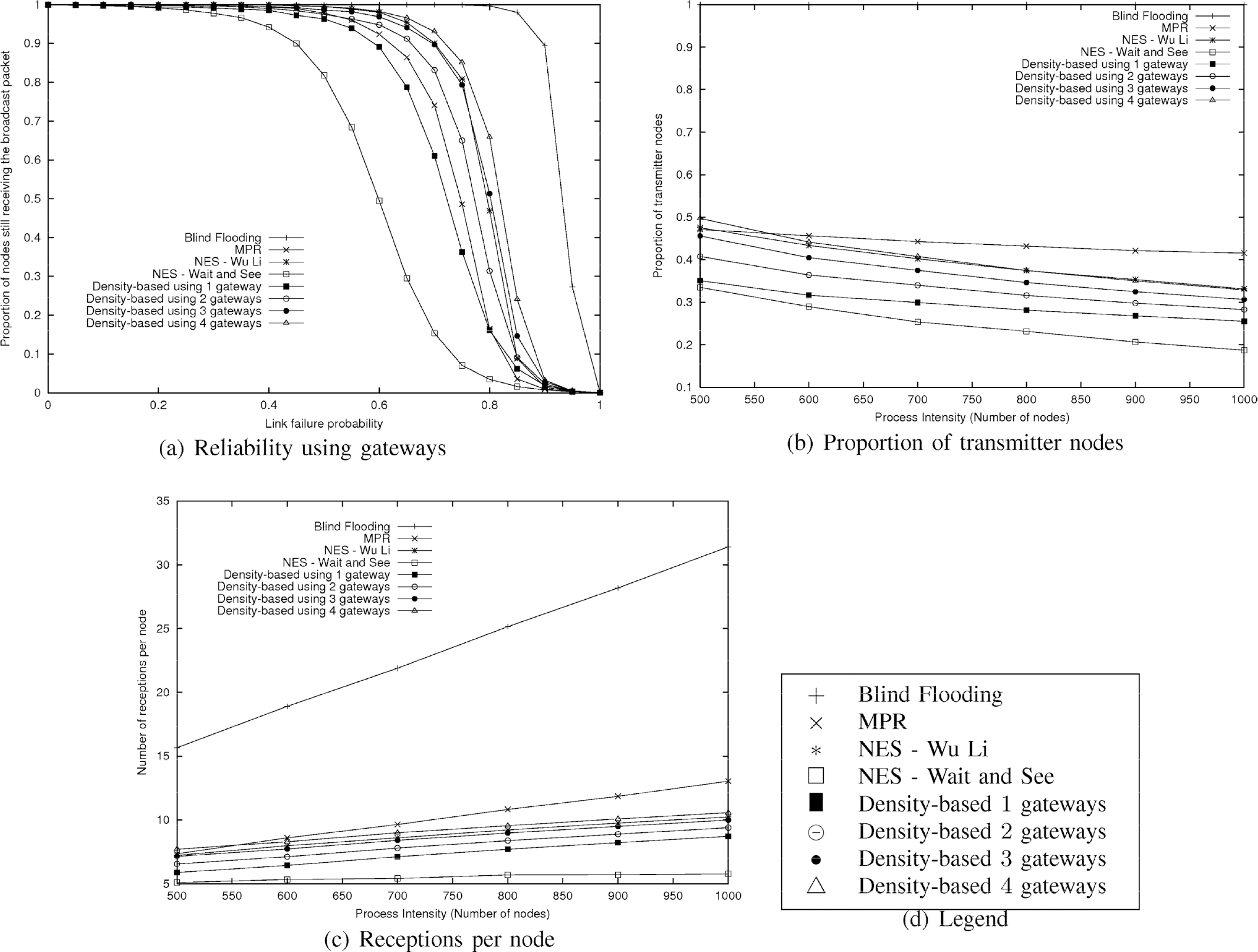
Reliability against link failures (a). Proportion of transmitters (b) and number of receptions per nodes (c) when using several gateways during a global broadcasting scheme.

VII. Conclusion and Perspectives

We have proposed a broadcasting scheme over a clustered topology for multi-hop wireless networks. We can thus obtain a double-use structure with low cost, as the maintenance is local and quasi-local. The cost is bounded by the tree depth which is a low constant. Moreover, two kinds of broadcasting tasks may be performed over it since we can perform global broadcastings in the entire network as well as broadcastings confined inside a cluster. Our proposed algorithm offers better results than some existing broadcasting schemes. More precisely, it saves more retransmissions since the number of internal nodes selected is lower (for both global and cluster-confined broadcastings). Moreover, the number of duplicated packets received is also lower. Note that reducing both emissions and receptions is an important factor when designing energy aware broadcasting protocols. Future works will be dedicated to investigate robustness of clustering-based broadcasting protocol in presence of node and link failures. Preliminary results tend to show that the confined broadcasting is more robust that the global one and thus we investigate more deeply the impact of the choice and number of gateways between clusters.

Footnotes

1

2

IPv6 addresses already use this concept of different broadcastings.

APPENDIX

We present here the proofs of Propositions 1 and .

References

Amis

Prakash

Vuong

, and Huynh

, “Max-Min D-cluster formation in wireless ad hoc networks,” in Proceedings of the IEEE INFOCOM, IEEE, Tel-Aviv, Isreal, March, 2000.

Busson

Mitton

, and Fleury

, “An analysis of the MPR selection in olsr and consequences,” in MED-HOC-NET 05, Porquerolles, France, June, 2005.

Cartigny

Ingelrest

, and Simplot-Ryl

, “RNG relay subset flooding protocol in mobile ad-hoc networks,” LIFCS, 253–265, 2003.

Chiang

I.I.

Liu

, and Gerla

, “Routing in clustered multihop, mobile wireless networks with fading channel,”, ICCS/ISPACS' 96, Singapore, November, 1996.

Dai

and Wu

, “Distributed dominant pruning in ad hoc networks,” In ICC'03, Anchorage, Alaska, USA, May, 2003.

Ephremides

Wieselthier

, and Baker

, “A design concept for reliable mobile radio networks with frequency hoping signaling.” in IEEE 75, 56–73, 1987.

Feeney

L. M.

and Nilsson

, “Investigating the energy consumption of a wireless network interface in an ad hoc networking environment,”, INFOCOM'01, Anchorage, Alaska, USA, April 2001.

Fernandess

and Malkhi

, “k-clustering in wireless ad hoc networks,”, POMC. Toulouse, France, 2002.

Garey

M. R.

and Johnson

D. S.

, Computers and intractability: A guide to the theory of NP-completeness. New York: W. H. Freeman & Company, 1979.

10.

Lim

and Kim

, “Multicast tree construction and flooding in wireless ad hoc networks,” in ACM MSWiM Workshop at MobiCom 2000, Boston, MA, USA, August, 2000.

11.

Lin

and Gerla

, “Adaptive clustering for mobile wireless networks,” IEEE JSAC. 15, 7, 1265–1275, 1997.

12.

Mitton

Busson

, and Fleury

, “Analysis of the self-organization in wireless multi-hops networks,” Research Report RR-5328, INRIA, 2004.

13.

Mitton

Busson

, and Fleury

, “Self-organization in large scale ad hoc networks.”, MED-HOC-NET 04, Bodrum, Turkey, June, 2004.

14.

Mitton

and Fleury

., “Efficient broadcasting in self-organizing multi-hop wireless network,” in Ad Hoc Now'05, Cancun, Mexico, 2005.

15.

Mitton

Fleury

Guérin-Lassous

, and Tixcuit

. “Self-stabilization in self-organized multihop wireless networks,” in WWAN'05, Columbus, Ohio, USA, June, 2005.

16.

Nikaein

Labiod

, and Bonnet

, “DDR-distributed dynamic routing algorithm for mobile ad hoc networks,” in MobiHoc, Boston, MA, USA, November, 2000.

17.

Qayyum

Viennot

, and Laouiti

“Multipoint relaying: An efficient technique for flooding in mobile wireless networks” in IIICSS'02, Hawaii, USA, January, 2002.

18.

Stojmenovic

Seddigh

, and Zunic

, “Dominating sets and neighbor climination-based broadcasting algorithms in wireless networks,” IEEE TPDS, 13, 1, January, 2002.

19.

Stojmenovic

and Wu

, “Broadcasting and activity scheduling in ad hoc networks,” IEEE Mobile ad Hoc Networking, pp. 205–229, 2004.

20.

Stoyan

Kendall

, and Mecke

, Stochastic Geometry and Its Applications, second edition. John Wiley & Sons, 1995.

21.

and Li

, “A dominating set based routing scheme in ad hoc wireless networks.” Telecommunication Systems, 13–36, 2001.

22.

and Lou

. “Forward node set based broadcast in clustered mobile ad hoc networks,” Wireless Communications and Mobile Computing, 3, 2, 141–154, 2003.

Efficient Broadcasting in Self-Organizing Sensor Networks

Abstract

Keywords

I. Introduction

II. Broadcasting in Multi-hop Wireless Networks

III. Previous Work and Main Objectives

Definition 1 (density)

A. Some Characteristics of the Clustering Algorithm

IV. Our Contribution

A. Gateway Selection

1) Mirror node selection

B. Broadcasting Heuristic

Proposition 1

Proposition 2

Discussion

1) Broadcasting over the whole network (global broadcasting)

Footnotes

1

2

APPENDIX

References