Sage Journals: Discover world-class research

Abstract

Distributed phased arrays have advantages over conventional arrays in many radar and communication applications. Additional advantages are realized by replacing the microwave beamforming circuit by a wireless network, thus forming a wirelessly networked distributed sensor array. This article examines various aspects of a distributed phased array that incorporates wireless beamforming. First, the fundamental array theory and digital signal processing are reviewed. Basic equations are presented and compared to simulations for a ship-based radar application. Next the basic array architecture is described and the critical techniques and components that are required to realize the design are discussed. Methods are introduced for time and phase synchronization, transmit-receive isolation, sensor location issues, and bandwidth and frequency dispersion.

Keywords

Distributed Phased Array Wireless Beamforming Radar Systems Communication Systems

1. Introduction

1.1. Phased Arrays and Conventional Beamforming

Phased array antennas are generally the antenna architecture of choice for most modern high performance radar and communication systems. Phased arrays consist of a collection of individual antennas that are geometrically arranged and excited (phased) so as to provide the desired radiation characteristics. Traditionally the elements are connected by a system of microwave transmission lines and power dividers (the beamforming network). In practice, the beamforming network can be physically large and heavy if there are a large number of elements. For example, it is not unusual for large ground or ship-based phased arrays to have tens of thousands of elements that are spaced about one-half of a wavelength at the operating frequency.

The array radiates or receives energy over a spatial angle (beam) that is measured by its half-power beam width (HPBW), which is often referred to as the field of view (FOV). The array beam can be scanned electronically by changing the relative phases of the elements. This approach permits rapid beam scanning and avoids the need to physically rotate the antenna. The antenna pattern sidelobes, which occur outside of the mainbeam and are generally undesirable, are suppressed by adjusting the relative power between the elements. In addition to weight and volume, another disadvantage of microwave circuits as beamformers is that they cannot be reconfigured or adjusted to change the sidelobe level. They also tend to be narrow band.

Figure 1a shows a conventional phased array with an analog beamformer that would be used in a radar or communication system. For simplicity a linear array is shown. In radar or communications, a message is encoded onto a baseband waveform that is up-converted to the operating band (for example, 2.45 GHz for a WLAN), then amplified and sent to the antenna. On receive, the signal out of the antenna is down-converted to baseband in the receiver and the received message reconstructed. Most phased arrays with analog beamformers are reciprocal; that is, capable of both transmitting and receiving.

Figure 1.

Phased array architectures.

A digital phased array architecture is shown in Fig. 1b. Typically each element has its own transmitter and receiver, combined into a transmit-receive (T/R) module. This eliminates the need for a beamforming network, but introduces other challenges. For example, the elements must be synchronized to common time and phase references in order to coherently transmit and then process the received signals from the individual elements. The receive processing is performed in a digital beamformer (computer processor). It is only recently that the low-cost miniaturized electronics and fast powerful computer processors have made this architecture practical for many applications.

1.2. Wireless Beamforming and its Advantages

A phased array is essentially a sensor network where the beamformer serves to collect and distribute signals from all of the sensors. Replacing the beamformer circuitry with a wireless network, as shown in Fig. 1c, yields all of the advantages of conventional wireless networks. The primary advantages are the ability to reconfigure and add elements, adaptability to the operational environment, and the ability to upgrade the system performance via software. The narrow band limitations of the beamforming circuit are removed, which potentially allows for wideband operation. Multiple radar, communications, and electronic warfare functions can be served by a single antenna having such an architecture.

In military applications the distributed and wireless characteristics enhance the survivability of the system. The fact that sensors can be distributed over a larger area, as opposed to concentrated in a small area, makes the system less vulnerable to a single hit [1]. The array processor can be reconfigured to compensate for element failures.

1.3. Applications and Challenges

The realization of a wirelessly beamformed phased array has several technological challenges. One is phase and time synchronization. Another is the rapid transfer of large amounts of data between the elements and the digital beamformer, and data processing speeds fast enough to permit real-time operation. In a dynamic environment where the elements are distributed on a flexible non-rigid surface, the position of the elements must be known to be within a fraction of a wavelength in order to compensate for phase errors and dispersion.

The concept of a distributed antenna array is not new. Long baseline interferometry is used in astronomy and employs many of the same principles as wireless beamforming [2]. Lee and Dorny [3] proposed a very large array using data collection from a fleet of ships, and proposed a “self-survey” technique to calibrate the system. Galati and Losquadro [4] described an air surveillance radar system where a constellation of satellites forms the radar array. Coherence and position location are achieved by optical measurements, and a communication system sends the elementary data to a master satellite for processing. Distributed array radar and its noise limited detection characteristics is described in [5].

A particular application of interest in this research is long range ballistic missile defense (BMD) radar stationed on a ship. An advantage of the wireless approach is that elements can be distributed over available areas on the surface of the ship. We refer to this as an opportunistic array (OA), in contrast to the conventional approach, where large areas on the ship surface are reserved for the array installation. The conventional approach limits the size of the array and also increases the ship structural requirements, because large areas of the ship surface are cut out to insert the array. Furthermore, the distribution of the elements over a large surface opens possibilities for integrating the individual elements into the surface as part of the material fabrication.

Another possible environment where the wirelessly beamformed opportunistic array has advantages is for rapid deployment of a system in emergencies; so-called “hastily formed networks.” For example, elements dispersed over the side of a hill or on the face of a building to function as an air traffic control (ATC) radar.

This paper describes a basic architecture for a wirelessly beamformed phased array, and examines the critical performance requirements and tradeoffs for hardware and software, concentrating on applications where the elements are distributed over the surface of a single platform or other relatively small area. There are other applications where individual platforms may constitute a single element of an array. Together they collectively comprise a distributed array that extends over an extremely wide area. An example is a swarm of unmanned air vehicles (UAVs) or a fleet of ships. There are many problems encountered in the wide area distributed array that are not present in the single platform case, or at least not to the same extent. Among them are the presence of range and angle ambiguities, geolocation of elements, wireless network range, wireless network vulnerability, and latency due to long range propagation delays.

In the following sections some of the critical aspects of the distributed wireless beamformed array are discussed. For the single platform with radar systems operating in the HF and VHF frequency bands (3–300 MHz), we can make the following assumptions:

The location of the elements will not deviate significantly (more than a fraction of a wavelength) from the ideal position. Therefore position measurement is not required.

The wireless channel is relatively stable and secure so that jamming and fading are not an issue.

There is sufficient power and thus power scavenging and conservation are not needed.

Section 2 presents formulas for the signal-to-noise ratio (SNR) of a distributed array and the array's expected gain, and sidelobe level. Section 3 discusses the array architecture and beamforming challenges in realizing the array performance. Section 4 discusses solutions to the key problems, including the timing and frequency synchronization issue, the transfer of data between the elements and the master controller, and the data processing and beamforming requirements. Some potential solutions are also presented. Finally, Section 5 contains a summary and conclusions.

2. Distributed Array Systems

2.1. Radar Range Equation for Distributed Radar

The general configuration for a distributed array radar and target is shown in Fig. 2. The monostatic condition occurs when the array elements are closely spaced compared to the range to the target. That is, the aspect angle of the target is the same for all elements. The multistatic case occurs when the elements are distributed over a wider area so that the aspect angle varies. Reference [5] derives the radar range equation (RRE) for various operating conditions and noise limited detection. The derivation is summarized here, with modification to include the phases of the received signals required for use in the digital beamforming.

Figure 2.

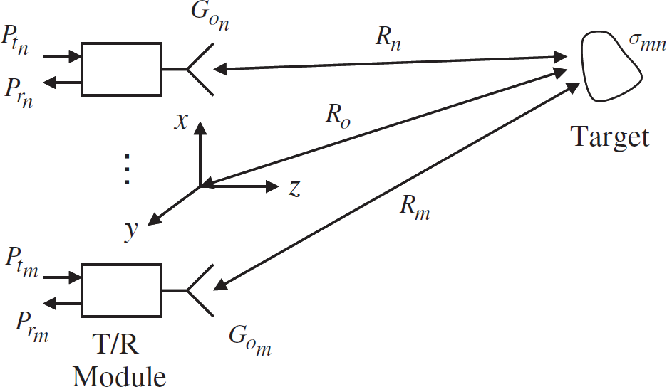
Distributed array radar geometry.

To simplify the derivation we neglect multipath, direct transmission between elements (mutual coupling) and assume that signals are all of one polarization. Furthermore, a single frequency continuous wave (CW) case is considered so that phasor notation can be used. The time convention exp(+jωt) is assumed and suppressed (ω = 2πf, f = frequency). The MKS system of units is used throughout unless otherwise noted.

If the target is in the far field of all elements, the time-averaged scattered power density (time-averaged quantities are denoted by an overbar) from the target at receive element m when element n is transmitting is given by [6]

{\bar{W}}_{m n}^{s} = (\frac{{\bar{P}}_{t_{n}} G_{o_{n}}}{4 π R_{n}^{2}}) (\frac{σ_{m n}}{4 π R_{m}^{2}})

(1) where

${\bar{P}}_{t_{n}}$ is the time-averaged power transmitted by element n

$G_{o_{n}}$ is the antenna gain of array element n, and

$G_{m n}$ is the bistatic RCS (shorthand notation for σ(θ _m , θ _n ) where θ _n denotes the incident aspect angle and θ _m the scattered aspect angle).

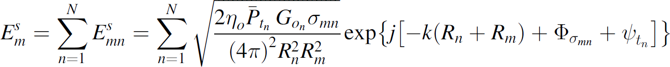
The amplitude of the phasor electric field at element m is obtained from the scattered power density

{\bar{W}}_{m n}^{s} = \frac{| E_{m n}^{s} |^{2}}{2 η_{o}}

(2) where

η_{o} = 377 Ω

is the intrinsic impedance of free space. The phase of the electric field at receive element m is determined by the path lengths (R_n + R_m) and any phase shift introduced by the target echo (

Φ_{σ_{m n}}

). Therefore, in polar notation

E_{m n}^{s} = \sqrt{\frac{2 η_{o} {\bar{P}}_{t_{n}} G_{o_{n}} σ_{m n}}{(4 π)^{2} R_{n}^{2} R_{m}^{2}}} \exp {[- k (R_{n} + R_{m}) + Φ_{σ_{m n}} + ψ_{t_{n}}]}

(3) where

k = \frac{2 π}{λ}

, λ the wavelength, and

ψ_{t_{n}}

is the phase added to element n to scan and focus the collective array beam.

The total scattered electric field received at element m from N transmitting elements is given by

E_{m}^{s} = \sum_{n = 1}^{N} E_{m n}^{s} = \sum_{n = 1}^{N} \sqrt{\frac{2 η_{o} {\bar{P}}_{t_{n}} G_{o_{n}} σ_{m n}}{(4 π)^{2} R_{n}^{2} R_{m}^{2}}} \exp {j [- k (R_{n} + R_{m}) + Φ_{σ_{m n}} + ψ_{t_{n}}]}

(4) where E^smn is the total phasor scattered electric field intensity from the target at receive element m due to transmit element n. The total received power is obtained by multiplying the incident power density by the effective area of the receive element m,

A_{e_{m}}

{\bar{P}}_{r_{m}} = A_{e_{m}} | \sum_{n = 1}^{N} \sqrt{\frac{{\bar{P}}_{t_{n}} G_{o_{n}} σ_{m n}}{(4 π)^{2} R_{n}^{2} R_{m}^{2}}} \exp {j [- k (R_{n} + R_{m}) + Φ_{σ_{m n}} + ψ_{t_{n}} + ψ_{r_{m}}]} | .

(5)

The term $ψ_{r_{m}}$ accounts for any phase added to the receive channel to focus and scan the beam.

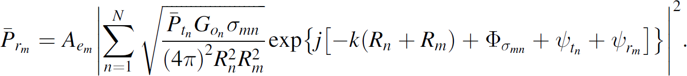
Finally, using the relationship between gain and effective area [7]

A_{e_{m}} = \frac{G_{o_{m}} λ^{2}}{4 π}

(6) and substituting it into Eq. (5), the total power received by element m is

{\bar{P}}_{r_{m}} = \frac{G_{o_{m}} λ^{2}}{(4 π)^{3}} | \sum_{n = 1}^{N} \frac{\sqrt{{\bar{P}}_{t_{n}} G_{o_{n}} σ_{m n}}}{R_{n} R_{m}} \exp {j [- k (R_{n} + R_{m}) + Φ_{σ_{m n}} + ψ_{t_{n}} + ψ_{r_{m}}]} |

(7)

Equation (7) is the most general form of the range equation for distributed array radar. For the conventional array with identical elements operating in a monostatic mode, equal transmit powers, and phase focusing to achieve coherence at the target, the following substitutions can be made:

Identical array elements; neglect mutual coupling: $G_{o_{m}} = G_{o_{n}} \equiv G_{o}$

Equal transmit powers: ${\bar{P}}_{t_{m}} = {\bar{P}}_{t_{n}} \equiv {\bar{P}}_{t}$

Monostatic scattering: $R_{n} = R_{m} \equiv R_{o}, σ_{m n} = σ_{o}, Φ_{σ_{m n}} \equiv Φ_{o} = 0$

Beam focused on the target: $ψ_{t_{n}} + ψ_{r_{m}} = k (R_{m} + R_{m}) \equiv 2 k R_{o}$

Thus, Equation (7) reduces to

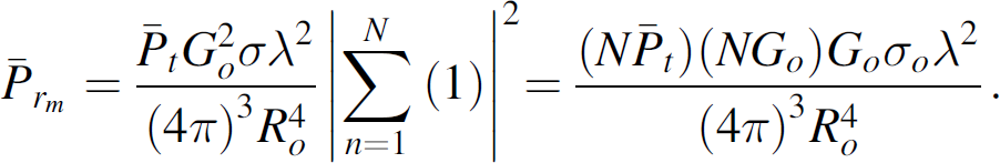
{\bar{P}}_{r_{m}} = \frac{{\bar{P}}_{t} G_{o}^{2} σ λ^{2}}{(4 π)^{3} R_{o}^{4}} {| \sum_{n = 1}^{N} (1) |}^{2} = \frac{(N {\bar{P}}_{t}) (N G_{o}) G_{o} σ_{o} λ^{2}}{(4 π)^{3} R_{o}^{4}} .

(8)

This result is consistent with the conventional radar range equation in [6]. For an N-element array, the total array transmit power is $N {\bar{P}}_{t}$ and the array antenna gain is NG_o.

2.2. Signal-to-Noise Ratio (SNR)

More important than the received power is the SNR at element m. For a focused calibrated array operating in a monostatic mode with thermal noise power $N_{o} = k_{B} T_{s} B$ [6]

{(\frac{S}{N_{o}})}_{m} = \frac{{\bar{P}}_{r_{m}}}{N_{o}} = \frac{G_{o_{m}} λ^{2}}{(4 π)^{3} k_{B} T_{s} B} {| \sum_{n = 1}^{N} \frac{\sqrt{{\bar{P}}_{t_{n}} G_{o_{n}} σ_{m n}}}{R_{n} R_{m}} \exp {- j 2 k R_{o}} |}^{2} .

(9)

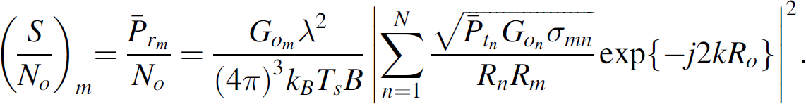
The system noise temperature is T_s, the bandwidth is B, and Boltzman's constant is $k_{B} = 1.38 \times 10^{- 23} J / K$ . If the radar uses coherent averaging of the returns from each element m, for M receive elements, this process involves adding the amplitude of M target signals that have coherent phase. The associated power of coherent summation is proportional to M². Thermal noise is usually assumed to be uncorrelated zero-mean Gaussian white noise of random amplitude and phase. The noise powers (variances) from M signals add to give the noise power of a single signal times M. The signal voltage adds (a factor of M₂ in power) and thus, the improvement in SNR is a factor of M over that of a single channel:

{(\frac{S}{N_{o}})}_{array} = M {(\frac{S}{N_{o}})}_{1} .

(10)

2.3. Array Pattern

The transmitting and receiving pattern of the array can be computed from the element locations and the orientations. For an observation point at infinity in the direction (θ, ϕ) the vectors from all elements to the observation point are parallel. The pattern factor F(θ, ϕ) for the array in three-dimensions with elements located at (x_n, y_n, z_n), n = 1, 2, 3, …, N is [7]

F (θ, ϕ) = \sum_{n = 1}^{N} A_{n} e^{+ j ψ_{n}} e^{+ j ψ_{s}} e^{+ j \vec{k} ∙ {\vec{r}}_{n}} E F_{n} (θ, ϕ)

(11) where

A_{n} e^{+ j ψ_{n}}

= complex coefficient of the n_th element that accounts for sidelobe control and corrections for all hardware non-idealities

$ψ_{s} = - k [(\sin θ_{S} \cos ϕ_{S}) x_{n} + (\sin θ_{s} \sin ϕ_{S}) y_{n} + (\cos θ_{S}) z_{n}]$ = beam scanning phase weights (θ_S, ϕ _S ) = scan angle

$\vec{k} = k (\hat{x} \sin θ \cos ϕ + \hat{y} \sin θ \sin ϕ + \hat{z} \cos θ)$ = position vector from the local array origin to element $n = {\vec{r}}_{n} = \hat{x} x_{n} + \hat{y} y_{n} + \hat{z} z_{n}$

EF_n = normalized electric field (voltage) element factor for the n^th element

In the case of a distributed array it is possible that flexure of the platform surface will introduce perturbations in the locations of the antenna elements. The position vector to element n then becomes:

{\vec{r}}_{n} = (x_{0 n} + Δ x_{n}) \hat{x} + (y_{0 n} + Δ y_{n}) \hat{y} + (Z_{0 n} + Δ z_{n})^{\hat{z}} = {\vec{r}}_{0 n} + δ {\vec{r}}_{n}

(12) where (x_0n, y_0n, z_0n) are the error-free element locations and (Δx_n, Δy_n, Δz_n) the deviations from the error-free locations. By assumption 1 of Section 1 these errors are neglected.

2.4. Element Factor

The element factor is the pattern of an individual element of the array. Normally it is the electric field or voltage pattern of the array element in its local environment. When elements are distributed over a complex doubly curved surface, the target may not be in the FOV of every element. For any given scan direction, only elements that have the target or signal source in their FOV contribute to the main lobe. Elements that do not contribute are turned off while the contributions of the remaining elements are used to determine the pattern factor.

The element factor can be expressed as:

E F_{n} = {\begin{cases} 1, & {\hat{n}}_{n} ∙ \hat{r} > 0 \\ 0, & otherwise \end{cases}

(13) where

{\hat{n}}_{n}

is the unit vector normal to the surface of the n^th element. Equation (13) describes an idealized hemispherical pattern (constant gain over the outward looking hemisphere). The actual form of EF is dictated by the specific element used in the array, and may be substantially different from element to element due to mutual coupling and interactions with local platform structure.

Figure 3 shows a distributed array on a ship surface. Each red “x” in the figure denotes the randomly selected location of an element. Figure 4 shows an azimuth pattern of an array of 1200 elements for a broadside scan angle 10 degrees above the horizon. For this particular scan angle, 780 elements contribute; for the remaining elements, the scan angle is not in their field of view.

Figure 3.

Ship model with 1200 randomly distributed array elements (the units are feet).

Figure 4.

Rectangular and polar plots of relative power pattern versus azimuth angle for broadside scan (ϕ _s = 90°, θ _S = 80°).

2.5. Directivity and Gain

The directive gain [7] can be written in terms of the normalized pattern factor F_norm (θ, ϕ):

D (θ, ϕ) = \frac{4 π}{\int_{0}^{2 π} \int_{0}^{π / 2} \frac{| F (θ, ϕ) |^{2}}{| F_{m a x} |^{2}} \sin θ d θ d ϕ} = \frac{4 π}{\int_{0}^{2 π} \int_{0}^{π / 2} | F_{norm} (θ, ϕ) |^{2} \sin θ d θ d ϕ} .

(14)

The maximum value of the directive gain is called the directivity, which is equal to the peak gain if the array has no losses. When losses are present the gain is the directivity multiplied by the efficiency [7]

G (θ, ϕ) = η D (θ, ϕ) = \frac{4 π A_{e}}{λ^{2}} | F_{norm} (θ, ϕ) |^{2}

(15) where η is the antenna efficiency (power radiated divided by power in,

0 \leq η \leq 1

) and A_e the effective area of the entire array.

2.6. Average Power Pattern and Sidelobe Level

The distributed array can be considered as a special case of either an aperiodic, random, or random thinned array [8]. The power pattern of an array can be determined by the product of the pattern factor (which is a voltage or electric field quantity) and its complex conjugate. Consider the expression for the array factor of N randomly spaced elements given in Eq. (11). Without loss of generality, assume that the array is properly phased to form the main lobe perpendicular to the array ( $ψ_{n} = 0$ and $e^{+ j ψ_{n}} + 1$ for all elements). The expected power pattern, $⟨ P ⟩$ , can be expressed as:

⟨ P ⟩ = ⟨ F F^{*} ⟩ = ⟨ \frac{1}{N^{2}} \sum_{n}^{N} \sum_{m}^{N} e^{+ j \vec{k} ∙ ({\vec{r}}_{n} - {\vec{r}}_{m})} ⟩

(16) where

⟨ \cdot ⟩

is the expectation operator. The position vectors are random variables with a known probability density function. Since the average of a sum equals the sum of the averages,

⟨ P ⟩ = \frac{1}{N^{2}} [N + ⟨^{+ j \vec{k} ∙ \vec{r}} ⟩ ⟨^{+ j \vec{k} ∙ \vec{r}} ⟩ (N^{2} - N)] = | ⟨ F ⟩ |^{2} (1 - \frac{1}{N}) + \frac{1}{N} .

(17)

The first term is the desired power pattern reduced by 1/N. The second term is an additive, angle-independent term of strength 1/N. Hence, the relationship between the expected power of the main lobe, $⟨ P_{mainlobe} ⟩$ , and the number of antenna elements is

⟨ P_{mainlobe} ⟩ = | ⟨ F ⟩ |^{2} (1 - \frac{1}{N})

(18) and the average sidelobe level relative to the mainlobe is

\frac{⟨ P_{sidelobe} ⟩}{⟨ P_{mainlobe} ⟩} = \frac{1}{N} .

(19)

In decibels, this ratio is 10 log₁₀(1/N).

The normalized power pattern of a random array can be determined by normalizing Eq. (18)

| F_{norm} (θ, ϕ) |^{2} = \frac{| ⟨ F ⟩ |^{2} (1 - \frac{1}{N})}{| ⟨ F ⟩ |^{2}} = 1 - \frac{1}{N} .

(20)

Combining Eqs. (15) and (20) gives

G (θ, ϕ) = \frac{4 π \forall_{e}}{λ^{2}} (1 - \frac{1}{N}) .

(21)

If we assume that the effective area of the individual elements are equal, then A_e of the array is proportional to the number of elements, N, and the relationship between the expected gain and the number of elements is

G (θ, ϕ) \propto N (1 - \frac{1}{N}) = N - 1.

(22)

Figures 5 and 6 compare the sidelobe levels and gain obtained by simulation for the ship model shown in Fig. 3 [9]. The gain was computed by numerical integration of Eq. (14). The trends predicted by Eqs. (19) and (22) are also plotted.

Figure 5.

Relationship between relative sidelobe level and number of active antenna elements (broadside scan, ϕ _S = 90° and θ _S = 80°, from [9]).

Figure 6.

Relationship between gain and number of active antenna elements (broadside scan, ϕ _S = 90° and θ _S = 80°, from [9]).

3. Description of the Array Architecture

3.1. Functional Block Diagram

A possible architecture of a wirelessly beamformed array is shown in Fig. 7 [10]. The array comprises of the central digital beamformer and controller that communicates wirelessly with hundreds or even thousands of array elements that are self-standing T/R modules. For clarity, only a single T/R module and array element is shown. For a ship application, the central digital beamformer and controller can be located below deck, while the array elements are randomly distributed over the ship surfaces.

Figure 7.

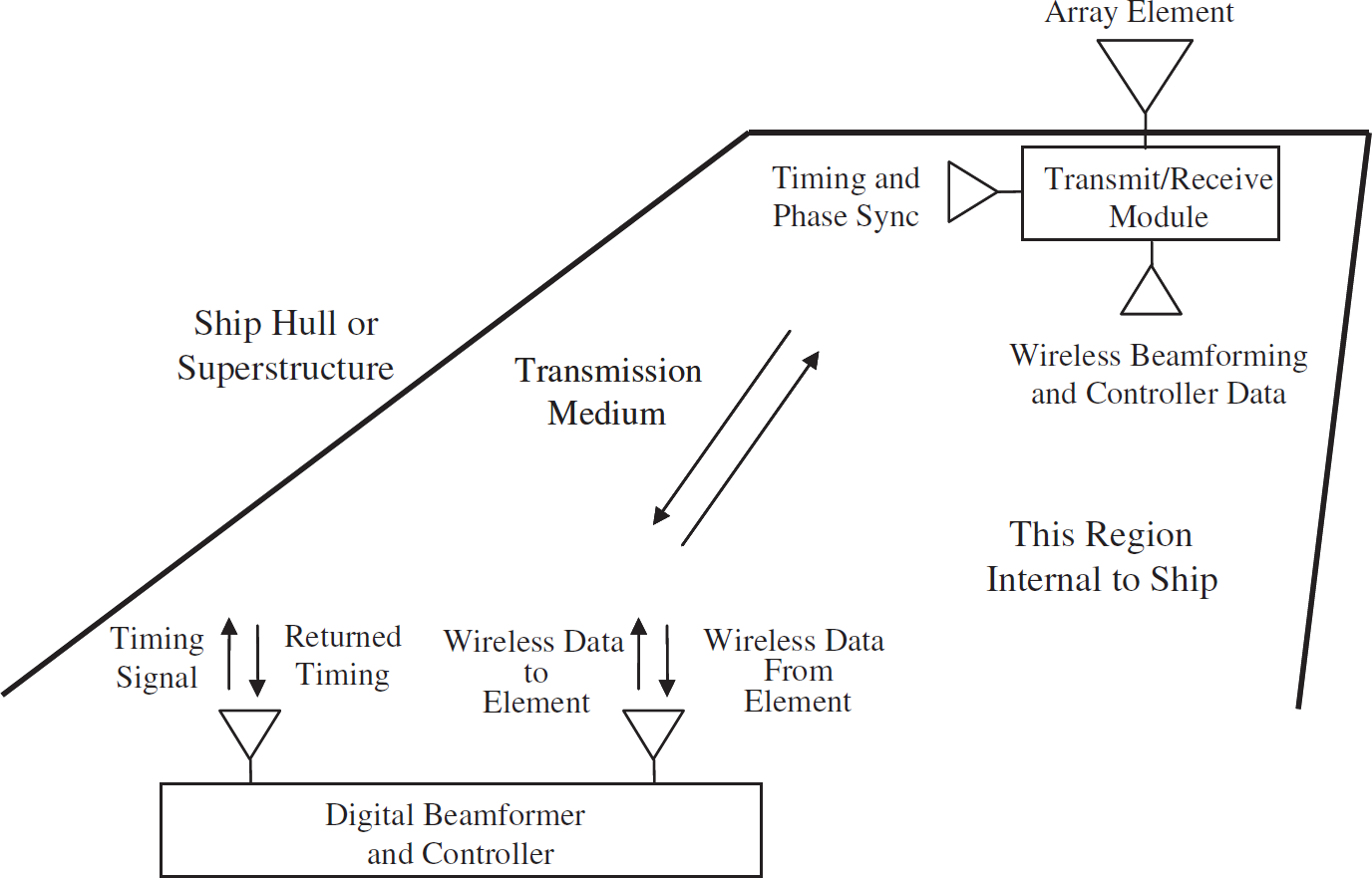
Wireless beamforming architecture.

The general operational concept of the array is as follows. The central digital beam-former and controller computes the beam control data (phase and amplitude weights for each element) and radar waveform parameters. These data, along with the time and phase synchronization signals, are passed wirelessly to all array elements.

A detailed architecture for each T/R module is shown in Fig. 8. At each array element, the digital baseband signal is generated by the direct digital synthesizer (DDS), converted to analog (with the D/A), and directly up-converted to the operating band and power amplified (PA). On receive, the signal is down-converted to baseband after low-noise amplification (LNA), quantized (with the A/D), and the in-phase (I) and quadrature (Q) data returned to the central digital beamformer and controller for processing.

Figure 8.

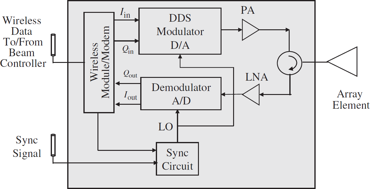
Details of a transmit-receive module.

The T/R module has a controller with some processing capability. There is a tradeoff to be made in this area. A sophisticated processor reduces the load on the central processor and the amount of data that needs to be transferred by the wireless network.

3.2. Digital Beamformer (DBF)

For the conventional phased array in Fig. 1a the signals are summed or split using power dividing networks. When a digital array operates in the transmit mode, the waveform is generated at each element, weighted and radiated at the proper time to achieve coherence and pulse overlap at the target. On receive the transmission lines in Fig. 1a perform the summation indicated in Eq. (11). In digital beamforming the sampled I and Q values from each element are passed to the signal processor where the array response can be computed for any desired scan and observation angle:

G (θ, ϕ) \propto N (1 - \frac{1}{N}) = N - 1.

(23)

The right hand side can be cast into an inner product of a vector of array weights and a vector of measured data. All of the quantities in Eq. (23) are functions of time. Therefore Eq. (23) could be written in time-sampled form, whereby I and Q are provided at discrete time intervals. A fundamental assumption in processing is that input signals are band limited to frequencies below one-half the sampling rate (Nyquist condition) [11]. The sampling frequency sets the performance of the analog-to-digital converters (ADCs) used in the T/R modules. Sampling at baseband, rather than at an intermediate frequency (IF), relaxes the sampling requirement. Note that the Nyquist condition also applies to sampled signals which are a function of distance or any other continuous independent variable.

A variety of signal processing functions can be performed by the computer in addition to DBF. Matched filtering, correlation, Dopper filtering, clutter cancellation, imaging, and interference rejection are among them [12 –14]. Reference [11] describes basic digital beamforming concepts and their relationship to filter design and spectral estimation.

Note that when normalized weights and inputs are used in Eq. (23) ( $(| A_{n} |, \sqrt{I_{n}^{2} + Q_{n}^{2}} \leq 1)$ ), and the incident wave direction coincides with the scan angle, a maximum output of N is obtained.

According to [15], important measures of DBF performance are dynamic range (DR), instantaneous bandwidth B, and the number of complex operations per second (COPS) performed by the DBF.

The DR of a DBF depends on

the number of bits in the ADC N_b,

the number of parallel elements N_e, and

the quantization noise.

The DR is given by 6N_b + 10logN_e and the number of COPS a DBF must handle is N_eB.

4. Critical Issues and Solutions

4.1. Time and Frequency Synchronization

Phase (frequency) and time references are broadcast to all elements. The frequency reference signal can be broadcast as a simple tone that is used to generate a local oscillator (LO) signal for use in the up and down conversion processes. A radio frequency (RF) pulse train can be used to establish time synchronization. Active synchronization techniques must be used to compensate for element dynamic motion and propagation channel changes. Generally synchronization is obtained by a feedback process whereby one fixed element serves as a reference (master), and the returned signals from other elements (slaves) are compared to the reference [16 –18].

A “brute force” technique for phase synchronization is to send a continuous wave (CW) signal to an element, which introduces a phase shift, and then returns it to the controller. The process is repeated for several phase values. Thus the proper phase shift is determined when the peak output of a detector is observed (actually it is more accurate to look for the null and add 180 degrees to the phase). This iterative process is repeated for all elements in the array. Although this is an inefficient approach, simulations have shown that adequate phase convergence can be achieved in just a couple of iterations [10]. In many applications phase errors up to a quarter of a wavelength (45 degrees) are tolerable—only a handful of phase values need to be examined for each element. Furthermore, when the propagation channel is quiet and stable, the phase variation with time will be small and slow. Figure 9 shows the residual phase error for one realization of an array of 100 randomly located elements with random initial phases. There were 872 iterations required to achieve synchronization. The simulation assumes 4 bits of phase shift are used (22.5 degrees) per iteration and quiescent (slowly varying) channel propagation characteristics. The residual phase error is within 1 bit; in this case ±11.25 degrees.

Figure 9.

Residual phase error after synchronization with 4-bit phase steps (from [10]).

The synchronization time can be reduced using more sophisticated techniques (i.e., orthogonal codes) that allow simultaneous measurements from all elements [19]. They require more complex hardware and signal processing capability.

Reference [20] describes a time synchronization technique that also involves sequential measurements using a master and slaves. It was shown that it takes N pulse repetition intervals (PRIs) to time synchronize an N-element array.

4.2. Frequency Dispersion and Time Varying Phase Weights

The waveforms transmitted and received have a bandwidth B centered on the carrier. The array must form a beam that stays fixed with frequency, so that all frequency components have a maximum pattern factor in the same spatial direction. However, if the phase to scan the beam ψ _s is a fixed constant and not true time delay, the beam will move with frequency as shown in Fig. 10a for a sixteen-element linear phased array [21]. The frequency scanning can be removed by using time-varying phase shifts, i.e., varying ψ _s with time, as described in reference [22]. Fig. 10b shows the patterns with time-varying phase shifts on transmit. In the simulation, the phase shift values are computed for a reference frequency of 1.7 GHz. The pattern factor is plotted from 0.8 GHz to 2.4 GHz for a uniform array of 16 isotropic elements spaced 0.08825 m. The fixed phase weights were computed based on the reference frequency and kept constant over all frequencies.

Figure 10.

Radiation patterns of a linear array using constant and time-varying phase weights (from [21]).

With time-varying phase weights, it is observed that the scan angle remains fixed. However, the beamwidth of the main beam for both types of weights increases when the frequency of the signal is lower than the reference frequency, and decreases when the frequency of the signal is higher than the reference frequency.

4.3. Transmit-Receive Isolation

For a radar or communications application the transmit and receive channels share a common antenna element, as shown in Fig. 8. Signals that “leak” directly from the transmitter to the receiver can mask returns from weak sources. There are two main components to the leakage:

the reverse signal that travels opposite the arrow directly from the transmitter, and

the antenna mismatch, which is the transmit signal reflected from the antenna input that travels through the circulator in the direction of the arrow, and arrives at the receiver.

If the circulator and antenna were ideal then neither of these signal components would be present. Possible solutions are:

Receiver blanking: A switch is added to the receive channel and opened when transmitting. Any signal that returns when the receiver is switched out is lost. This is referred to as eclipsing.

Improve hardware performance: Circulators with high isolation are expensive and large. Reducing the antenna mismatch has its limits, especially in real environments.

Leakage power cancellation: The leakage power travels a fixed path and arrives with known amplitude at a known time. The transmit signal can be sampled and stored, then subtracted from the received signal. This technique has been used successfully in CW and frequency modulated CW (FMCW) radars [23, 24].

4.4. Wireless Network Architecture

The transfer of data, commands, and synchronization signals is accomplished wirelessly. The proposed communication architecture is shown in Fig. 11. At regular intervals, each array element will send Position Location Data to the central digital beamformer and controller. As mentioned previously, for many applications the position errors can be ignored, and this data need not be provided. With knowledge of the element locations, the processor calculates the appropriate digital amplitude and phase weights for each array element for beamforming, and broadcasts this information to all array elements in the Waveform and Control Data. The distribution of the LO (required by the modulator and demodulator) and the timing signal REFCLK (required for the DDS) are distributed and processed as described in Section 4.1. Each T/R module incorporates hardware (Sync Circuit in Fig. 8) for performing the synchronization. The Phase Synchronization Control Data is used to phase synchronize all the array elements (i.e., switch in phases as described previously). The amplitude and phase weighted waveform is then modulated, amplified, and transmitted. On receive, echo signals are demodulated and the Target Return Data sent to the central digital beamformer and controller for processing.

Figure 11.

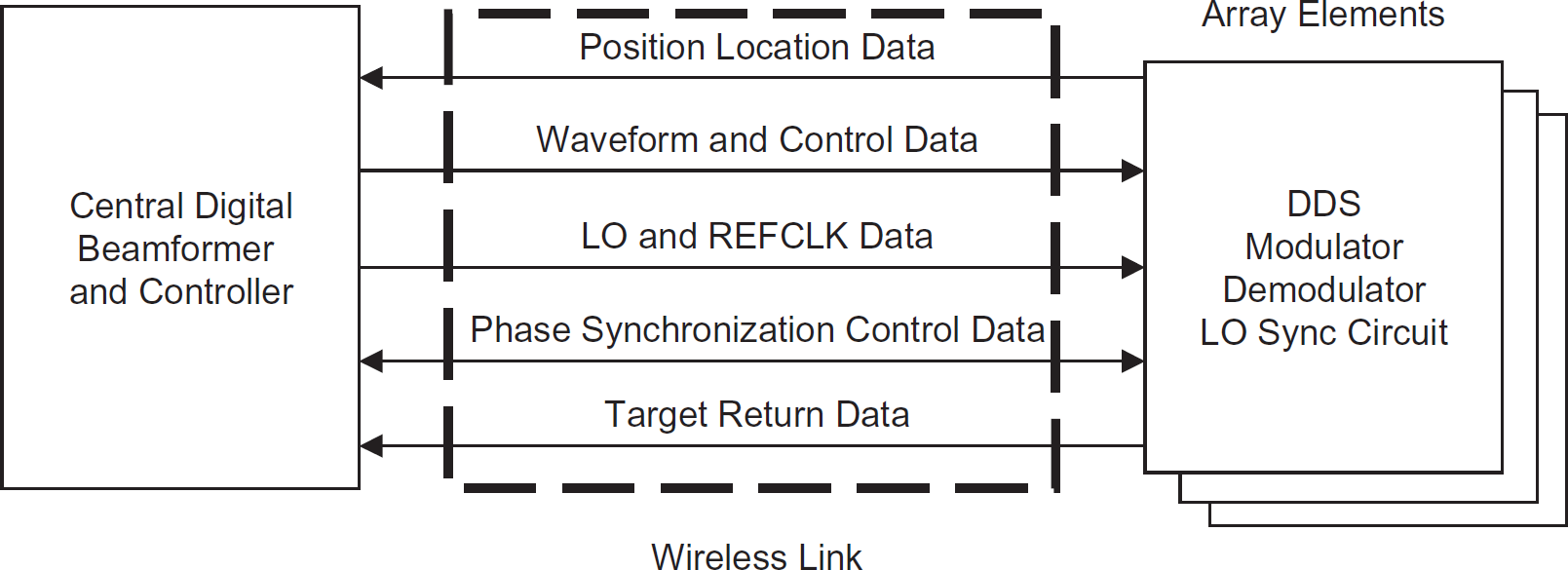
Data transfer for wireless beamforming (from [10]).

The one-to-many no hop configuration described above provides the most flexibility in the array distribution. There are other possible network configurations that combine wireless links and hardwired segments. For example, regions of the array that have a high density of elements could share a common wireless access point, which is connected to the individual elements via a local hardwire hub and spoke topology. Clusters of elements can be provided with additional processing capability to reduce the amount of data flow and computational demand on the central processor.

4.5. Real-Time Processing and Scheduling

As a first cut at estimating the array's data rate requirement, reference [10] identified a total of eight bits for waveform control, phase weighting, and phase synchronization commands. The amount of transmit data that needs to be sent is small compared to the receive channel. Transmission requires the amplitude and phase weights (I and Q for the modulators) and waveform parameters (pulse width and PRI, or FMCW sweep rate and frequency excursion). The waveforms themselves are stored in the DDS and simply read out at the rate specified by the transmit parameters.

The receive channel data rate requirement is dominated by the resolution of the ADC. For example, it is common for quadrature demodulator boards to use differential signal outputs (two for I and two for Q). If a four-channel ADC is used, sampling simultaneously at R_s samples/s with a resolution of N_b bits, the required bit rate is R_b = 4 X N_b X R_s bps per array element. For an N-element array, with 16 bit ADCs sampling at 100 kS/s (which is a very low rate for a radar), the network needs to handle a total data rate of 6.4N Mbps.

Clearly commercially available IEEE 802.11g standard wireless links (data rates up to 54 Mbps) will be taxed with only a handful of elements. Furthermore, this assumes that selective scheduling is used so that transmit and receive data exchanges do not occur simultaneously.

Data rate is a major challenge for wireless beamforming and solutions are limited. More processing or hardware capability can be added at the element level to reduce the amount of data transferred. For example, if the differential signals are combined at each element (which requires additional electronics), the data rate can be reduced by a factor of two. Other possible solutions are multiple wireless channels covering a range of frequencies, multiple input multiple output (MIMO) systems, or moving to optical links, which can provide data rates in the range of gigabits per second.

Since the sampling rate f_s has the most direct impact on data rate, any possible reduction in the sampling frequency should be considered. In some situations undersampling (sub-Nyquist sampling rate) can be used [25]. In addition to reducing the data rate, it can also increase the instantaneous bandwidth, and allows a fast Fourier transform (FFT) processing speed that need not match the bandwidth.

Another consideration is sampling loss [26] which occurs when the baseband signal is sampled and digitized by the ADC. This is the difference between the sampled value and the maximum pulse amplitude. For probabilities of detection of 0.90 and false alarm of 10⁻⁶, Skolnik [6] states that the sampling loss is 2 dB if sampling once per pulse width and 0.5 dB for two samples per pulse and 0.2 dB for three samples per pulse. The number of samples per pulse N_s is related to f_s, duty cycle D_u, pulse width τ, and pulse repetition frequency (PRF) f_p by

N_{s} = f_{s} \times D_{u} \times \frac{1}{f_{p}} = f_{s} τ .

(24)

With a sampling rate of 100 kS/s, to keep the sampling loss low with at least three samples per pulse, τ should not be smaller than 3×10⁻⁵s.

The ADC is a critical component that affects several aspects of the system performance. The dynamic range, in dB, of an ADC is given by 20log(2 ^N _b — 1) [26]. The dynamic range of the ADCs should be consistent with the selection of minimum SNR and dynamic range of the receiver. Another ADC effect that needs to be considered is its spurious response [25].

5. Summary and Conclusions

Distributed phased arrays employing wireless beamforming have the potential to fundamentally change the deployment of antennas for radar, communication, and electronic warfare applications. This paper has examined several critical issues in the design and operation of wirelessly beamformed arrays, and presented techniques that can be used to solve the major problems in realizing such arrays. The primary obstacle is the high data rate required for the wireless network, compared to the capability of today's wireless systems. However, solutions are on the horizon with new wireless systems that have the potential for gigabit per second data rates [27].

Given the current state-of-the-art in wireless networks, a small array (≤ 10 elements) using wireless beamforming is achievable. Many of the techniques have been demonstrated in the laboratory, including wireless LO distribution [28], transmit waveform generation via DDS, and up conversion [29], and development of a T/R module at 2.4 GHz using off the shelf components [30]. The integrated microwave circuitry, electronics, computer processing, and control technology are currently capable of supporting a small wirelessly beamformed array.

There are several other secondary issues that were neglected in the current discussion that must eventually be addressed. Self interference can occur, especially if high power is used on transmit. Jamming of the wireless network is a concern in a military environment. If the wireless network is disabled then the entire system is incapacitated. Harsh propagation channels and fading may have the same effect, reducing the data rate to the point where antenna performance degrades significantly. Finally, in many instances, real time geolocation of the array elements will have to be conducted so that position errors can be compensated for in the processing.

References

Ball

R. E.

, The Fundamentals of Aircraft Combat Survivability Analysis and Design, 2nd edition, AIAA Education Series, 2003.

Steinberg

B. D.

, Microwave Imaging with Large Antenna Arrays: Radio Camera Principles and Techniques, Wiley, 1983.

Lee

Dorny

C. N.

, “A broadcast reference technique for self-calibrating of large antenna phased arrays,” IEEE Trans. on Antennas and Prop. vol. 37, no. 8, August 1989.

Galati

Losquadro

, “Distributed-array radar system comprising an array of interconnected elementary satellites,” U.S. Patent 4,843,397, June 27, 1989.

Hermiller

Belyea

Tomlinson

, “Distributed array radar,” IEEE Trans. on Aerospace and Elect. Systems, vol. AES-19, no. 6, Nov. 1983, pp. 831–839.

Skolnik

M. I.

, Introduction to Radar Systems, 3rd edition, McGraw-Hill, New York, 2001.

Stutzman

W. L.

Thiele

G. A.

, Antenna Theory and Design, 2nd edition, Wiley, New York, 1998.

Steinberg

B. D.

, Principles of Aperture and Array System Design, Wiley, New York, 1976.

Tong

C. H.

, “System study and design of broad-band U-slot microstrip patch antennas for aperstuctures and opportunistic arrays,” Master's Thesis, Naval Postgraduate School, Monterey, California, December 2005.

10.

Yong

, “Sensor synchronization, geolocation and wireless communication in a shipboard opportunistic array,” Master's Thesis, Naval Postgraduate School, Monterey, California, March 2006.

11.

Dudgeon

D. E.

, “Fundamentals of digital array processing,” Proc. of the IEEE vol. 65, no. 6, pp. 898–904, June 1977.

12.

Chen

C. C.

Ling

, Time-Frequency Transforms for Radar Imaging and Signal Analysis, Artech House, 2002.

13.

Levanon

, Radar Principles, New York: John Wiley and Sons, 1988.

14.

Peebles

P. Z.

, Radar Principles, New York: Wiley Interscience, 1998.

15.

Fourikis

, Advanced Array Systems, Applications and RF Technologies, pp. 336–339, Academic Press, 2000.

16.

Adams

R. T.

, “Beam tagging for control of adaptive transmitting arrays,” IEEE Transactions on Antennas and Propagation, vol. AP-12, pp. 224–227, March 1964.

17.

East

T. W. R.

, “A self-steering array for the SHARP microwave-powered aircraft,” IEEE Transactions on Antennas and Propagation vol. 30, no. 12, p. 1565, December 1992.

18.

Taheri

S. H.

Steinberg

B. D.

, “Tolerance in self-cohering antenna arrays of arbitrary geometry,” IEEE Transactions on Antennas and Propagation, vol. AP-24, no. 5, pp. 733–739, September 1976.

19.

Silverstein

, “Applications of orthogonal codes to the calibration of active phased array antennas for communications satellites,” IEEE Trans. on Signal Proc. vol. 45, no. 1, January 1997.

20.

Attia

E. H.

Abend

, “An experimental demonstration of a distributed array radar,” IEEE Proceedings, 1991.

21.

Ong

C. S.

, “Digital phased array architectures for radar and communications based on off-the-shelf wireless technologies,” Master's Thesis, Naval Postgraduate School, Monterey, California, December 2004.

22.

Plumb

R. G.

, “Antenna array beam steering using time-varying weights,” IEEE Trans. on Aerospace and Electronic Systems vol. 27, no. 6, pp. 861–865, Nov. 1991.

23.

Beasley

P. D. L.

Stove

A. G.

Reits

B. J.

, “Solving the problems of a single antenna frequency modulated CW radar,” Record of the 1990 IEEE International Radar Conference, Vol. Iss, pp. 391–395, 7–10 May 1990.

24.

Kaihui

Yuanxun

E. W.

, “Real-time DSP for reflected power cancellation in FMCW radars,” IEEE Proceedings, 2004.

25.

Tsui

, Digital Techniques for Wideband Receivers, 2nd edition, Artech House, 2004.

26.

Gray

, Application Notes, “ABCs of ADCs,” National Semiconductor, 2003.

27.

Larry

Garfield

, “Siemens claims 1 Gbps wireless transmission,” InfoSync, 13 December 2004, at http://www.infosyncworld.com/news/n/5630.html, accessed January 2007.

28.

Yong

Y. C.

, “Receive channel architecture and transmission system for digital array radar,” Master's Thesis, Naval Postgraduate School, Monterey, California, December 2005.

29.

Ong

, “Commercial off the shelf direct digital synthesizers for digital array radar,” Master's Thesis, Naval Postgraduate School, Monterey, California, December 2005.

30.

Yeo

E. C.

, “Wirelessly networked opportunistic digital phased array: system analysis and development of a 2.4 GHz demonstrator,” Master's Thesis, Naval Postgraduate School, Monterey, California, December 2006.

Distributed Phased Arrays and Wireless Beamforming Networks

Abstract

Keywords

1. Introduction

1.1. Phased Arrays and Conventional Beamforming

1.3. Applications and Challenges

2. Distributed Array Systems

2.1. Radar Range Equation for Distributed Radar

3.1. Functional Block Diagram

4.1. Time and Frequency Synchronization

4.4. Wireless Network Architecture

References