Sage Journals: Discover world-class research

Abstract

Sensor networks naturally apply to a broad range of applications that involve system monitoring and information tracking (e.g., airport security infrastructure, monitoring of children in metropolitan areas, product transition in warehouse networks, fine-grained weather/environmental measurements, etc.). Meanwhile, there are considerable performance deficiencies in applying existing sensornets in the applications that have stringent requirements for efficient mechanisms for querying sensor data and delivering the query result. The amount of data collected from all relevant sensors may be quite large and will require high data transmission rates to satisfy time constraints. It implies that excessive packet collisions can lead to packet losses and retransmissions resulting in significant energy costs and latency. In this paper we provide a formal consideration of a Data Transmission Algebra (DTA) that supports application-driven data interrogation patterns and optimization across multiple network layers. We use a logical framework to specify DTA semantics and to prove its soundness and completeness. Further, we prove that DTA query execution schedules have the key property of being collision-free. Finally, we describe and evaluate an algebraic query optimizer performing collision-aware query scheduling that both improve the response time and reduce the energy consumption.

Keywords

Wireless sensor networks Cross-layer techniques Query optimization Algebraic optimization Wireless communications

1. Introduction

Recent advances in wireless communications and microelectronics have enabled wide deployment of smart wireless sensor networks (WSNs). Such networks will support a broad range of scientific, commercial, or security applications that require information tracking. Meanwhile, there are considerable performance deficiencies in applying existing WSNs in critical monitoring applications. As an example, consider Structural Health Monitoring (SHM) in which a wireless sensor network is deployed to monitor the structural integrity of a building or a ship [9, 24, 25]. As such tasks are characterized by considerable network load, excessive packet collisions lead to packet losses and retransmissions resulting in significant energy costs and latency. For example, the successful packet delivery ratio in 802.15.4 networks can drop from 95% to 55% as the load increases from 1 packet/sec to 10 packets/sec [16, 33]. Meanwhile, the sensors in an SHM system can generate up to 6 packets/sec of vibration data. As reported in [24, 25] the average residence time for 1 packet in a medium scale multi-hop sensor network could be tens of seconds. When this rate increases to 2 packets/sec per sensor, the network collapses. Under high traffic load, sensor nodes quickly run out of energy due to collisions and consequently the increased death of the sensors decreases the timeliness and the quality of data.

Several techniques have been proposed to alleviate the problem of network load and limited power at the network level such as energy-efficient routing and clustering [4, 14, 15, 27]. Sensor database research has also investigated sensor query processing strategies to minimize query response time and reduce energy consumption. Such strategies are sampling (e.g. [18]), prediction (e.g. [10, 7]), approximation (e.g. [5]), and in-network query processing (or aggregation) (e.g. [1, 3, 18, 23]). Sensor databases extend database technology to monitoring and query processing over sensor networks [1, 2, 26]. These include both language extensions to SQL and new query execution strategies. Typical sensor query execution maps into a tree-like data delivery pattern where a responding sensor node sends its data to a neighbor node which then transmits it further to the next node towards the requesting node (the root). Looking at these techniques in terms of traditional databases, we realize that these efforts primarily focus on one of the two main elements for improving the interactive performance of queries, namely query optimization, which decides the dependencies between the query operators (the query plan). The other main element is scheduling that decides the order of execution of query operators (concurrency control). Scheduling affects both energy consumption and response time.

Our research, on one hand enhances all the above existing approaches while on the other hand it offers the only solution for the timeliness and quality of data when none of these techniques are applicable. Specifically, we formally study query scheduling in sensor databases that combines both the data processing at sensor nodes and data transmission among sensor nodes. We develop an optimization framework and a Data Transmission Algebra (DTA) that allows an optimizer to utilize lower network layer protocols in scheduling sensor database queries [29, 30, 38]. In particular, DTA can capture the information about how the medium access control (MAC) layer operates while processing sensor queries. That is, the DTA can uniformly capture the structure of data transmissions, their constraints/conflicts, and their requirements. Our framework enables both qualitative analysis and quantitative cost-based optimization of sensor queries. Further, it allows the automatic generation and evaluation of alternative routing trees for a given set of queries and network configurations. Using our framework, we have been able to develop novel cross-layer optimization techniques. An example of such an optimization is collision-aware query scheduling [29] that minimizes simultaneous transmissions that interfere with each other. As opposed to other schemes which assume that the MAC layer handles collisions in an appropriate manner, our collision-aware query scheduling reduces the amount of retransmissions and thus saves time and energy.

In this paper, we present a formal study of our framework. We consider the soundness and completeness of our algebra and show that the schedules derived using DTA have the key property of being collision-free. Specifically, in Section 2, we describe our system model and introduce the relevant wireless data communication background. In Section 3, we informally introduce DTA and its application to cost-based query scheduling. Section 4 specifies the DTA signature together with a basic set of DTA inference rules (DTA theory). In Section 5, we use a logical framework to specify DTA semantics. It should be noted that many a formalism exists that can be used to consider the soundness and completeness of our algebra (e.g., λ-calculus). We have chosen the logical formalism, which is naturally to utilize within the database community. In Section 6 we study and prove the soundness and completeness of DTA, and show that valid DTA schedules are collision-free. Sections 7 and 8 elaborate on the implementation of our algebraic optimizer and provide its experimental evaluation. Section 9 concludes.

2. System Model

We assume that a query optimizer executes at the base station along with other utilities such as data mining for cost-effective and model-driven data acquisition [DGMHH04]. For a given query or data acquisition model, our query optimizer selects the query routing tree with optimal response time and energy consumption. A query optimizer generates alternative query schedules taking into consideration the current topology of stationary sensor nodes, the applications' coverage requirements, and the Collision Domains (CDs) of the sensor nodes, which we explain next.

In general, the transmissions between sensors are ad hoc dependent on the query and require the use of a medium access control (MAC) layer to handle transmissions on the same medium. If we assume that all sensor nodes use the same frequency band for transmission, two transmissions that overlap will get corrupted (collide) if the sensor nodes involved in transmission or reception are in the same collision domain CD(ni, nj) defined as the union of the transmission ranges of ni and nj. Figure 1 elaborates on the concept of collision domains in a typical wireless network such as IEEE 802.15.4 [33] and illustrates how collisions are handled in such a network. Consider two nodes n1 and n2 that wish to communicate. In Fig. 1, nodes n1, n2, n3, and n4, n5, and n6 are in the same collision domain. This implies that when n1 and n2 are communicating, n3, n4, n5, and n6 cannot participate in any communications. A typical wireless network handles collisions using carrier sense multiple-access with collision avoidance (CSCMA-CA) [6]. In general, before starting a transmission, nodes must sense the channel for a predetermined amount of time (waiting time). If the channel is busy, the nodes wait for the predetermined amount of time after the channel becomes free. In addition, nodes back off for a random time to avoid the possibility that two or more nodes transmit at the same time after the waiting period. For this entire period, the node must sense the channel and this consumes energy. Each packet also needs to be acknowledged by the receiver since wireless channels are unreliable.

Figure 1.

Collision domain of two communicating sensors.

3. Algebraic Query Optimization using DTA

In related research [29, 30] we introduced an algebraic query optimization technique for sensor networks. We developed a Data Transmission Algebra(DTA) that allows a query optimizer to generate query routing trees to maximize collision-free concurrent data transmissions.

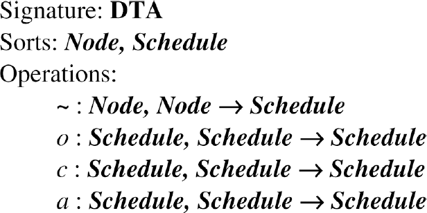
The DTA consists of a set of operations that take transmissions between wireless sensor nodes as input and produce a schedule of transmissions as their result. A one-hop transmission from a source sensor node ni to a destination node nj is called elementary transmission (denoted ni∼nj). Each elementary transmission ni∼nj is associated with a collision domain CD(ni, nj) as defined above. A transmission schedule is either an elementary transmission, or a composition of elementary transmissions using one of the operations of the DTA. The basic DTA includes three operations that combine two transmission schedules A and B:

o (A,B). This is a strict order operation, that is, A must be executed before B.

c (A,B). This is a non-strict order operation, that is, either A executes before B, or vice versa. Thus, c(A,B) ≡ (o(A,B) or o(B,A)).

a (A,B). This is an overlap operation, that is, A and B can be executed concurrently.

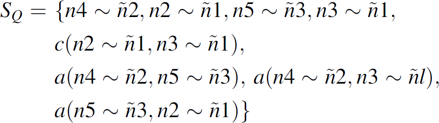
For an example of the DTA operations consider the query tree in Fig. 2 which was generated for some query Q. It shows some DTA specifications that reflect basic constraints of the query tree. For instance, operation o(n4∼n2, n2∼n1) specifies that transmission n2∼n1 occurs after n4∼n2 is completed. This constraint reflects a part of the query tree topology. Operation c(n2∼n1, n3∼n1) specifies that there is an order between transmissions n2∼n1 and n3∼n1 since they share the same destination. However, this order is not strict. Operation a(n4∼n2, n5∼n3) specifies that n4∼n2 can be executed concurrently with n5∼n3, since neither n3 nor n5 belongs to CD(n4,n2), and neither n4 nor n2 are in CD(n5,n3).

Figure 2.

Example of a query tree for some query Q and DTA specification.

Each operation of the DTA specification defines a simple transmission schedule that consists of two elementary transmissions. The DTA introduces a set of transformation rules [29, 30] that can be used to generate more complex schedules. Figure 2 shows an example of a complete schedule that includes all elementary transmissions of the query tree. Figure 2 also shows the initial DTA specification reflecting basic constraints of the query tree. The initial specification consists of a set of elementary transmissions reflecting the tree topology imposed by the query semantics, as well as order and overlap operations over the elementary transmissions. Non-strict order constraints can be derived from the initial specification. Figure 3 illustrates a query tree with different topology. The initial DTA specification of the second tree includes only two potentially concurrent transmission pairs.

Figure 3.

Impact of sensor topology on initial DTA specification.

Using an initial DTA specification, a cost-based query optimizer identifies DTA schedules with acceptable query response time and overall energy consumption. Implementation and experimental evaluation of our optimizer are provided in Sections 7 and 8. Next, we consider the soundness and completeness of the DTA, and prove that the DTA query execution schedules have the key property of being collision-free. In order to do that, first we will introduce formal specification of the DTA syntax and semantics.

4. DTA Theory

In this section we introduce a DTA theory consisting of the DTA signature and DTA inference rules [8]. The DTA signature specifies basic DTA syntax, while DTA inference rules represent transformations of the well-formed DTA terms. The DTA signature specification is presented in Fig. 4. It includes a set of sorts together with operations defined on them. The DTA signature includes two sorts Node and Schedule. Elementary transmission (denoted ∼) is a DTA operation that takes two nodes as input and outputs a schedule. The rest of the DTA operations (o, c, a) map two input schedules to an output schedule.

Figure 4.

DTA Signature.

In order to introduce DTA inference rules we extend the basic DTA signature with a secondary operation subs, which for a given DTA schedule returns all its sub-schedules. The subs operation is specified as follows:

subs : Schedule → P(Schedule),

where P(Schedule) denotes the power set of schedules. The following equations complete the specification of subs:

subs(XỸ) = {XỸ}.

subs(comp(S1, S2)) = {comp(S1, S2)} ∪ subs(S1) ∪ subs(S2),

where comp denotes any of DTA operations o, c, or a.

DTA inference rules are represented in Fig. 5. A DTA inference rule Premise → Conclusion reflects the fact that there is a one step inference from Premise to Conclusion. For example, using rule 1 (order introduction) we can infer a strict order of two elementary transmission if the destination node of the first transmission is also a source node of the second transmission. Rule 5 generates a strict order of DTA schedules X and S if there exists a sub-schedule S_i of the schedule S such that o(X,S_i) can be generated by the DTA rules. In order to infer a(X,S), we should be able to infer a(X, S_i) for all sub-schedules S_i of the schedule S.

Figure 5.

Basic DTA Inference Rules.

4.1. Definition 1 (DTA Inferability)

A DTA schedule t is inferable from a set of DTA schedules S (denoted $S | - t$ ) iff either t ∊ S, or t can be generated from S via finite applications of the DTA inference rules.

Example 1. Consider the following set of DTA schedules:

S = {n 4 \sim \tilde{n} 2, n 2 \sim \tilde{n} 1, n 5 \sim \tilde{n} 3, n 3 \sim \tilde{n} 1, a (n 4 \sim \tilde{n} 2, n 5 \sim \tilde{n} 3), a (n 4 \sim \tilde{n} 2, n 3 \sim \tilde{n} 1)},

which is a subset of the initial DTA specification from Fig. 2. We can infer from S the following schedule:

a (n 4 \sim \tilde{n} 2, o (n 5 \sim \tilde{n} 3, n 3 \sim \tilde{n} 1)),

using rules 1 and 8:

\begin{matrix} n 5 \sim \tilde{n} 3, n 3 \sim \tilde{n} \to_{r u l e 1} o (n 5 \sim \tilde{n} 3, n 3 \sim \tilde{n} 1), \\ a (n 4 \sim \tilde{n} 2, n 5 \sim \tilde{n} 3), a (n 4 \sim \tilde{n} 2, n 3 \sim \tilde{n} 1) \to_{r u l e 8} a (n 4 \sim \tilde{n} 2, o (n 5 \sim \tilde{n} 3, n 3 \sim \tilde{n} 1)) . \end{matrix}

5. DTA Semantics

We provide a logic-based specification of DTA semantics using Prolog-like Horn clauses [GZ02]. A predicate looks as follows: p(t1,t2, …, tn), where p is a predicate name of arity n, each ti is a term, and (t1,t2, …, tn) is a tuple. A term is a constant or a variable, or a complex term constructed using function symbols. A name starting with a capital letter signifies a variable. A rule is a statement of the form

p : - q 1, q 2, \dots, q n,

where p and qi are predicates, p is the rule head, and the conjunction q1, q2, …, qn is the rule body. A rule with an empty body is called a fact. A rule may be used to define the predicate p, so that p holds whenever q1, …, qn all hold. For example, the following rule defines that X is a grandparent of Y if X is a parent of Z and Z is a parent of Y:

g r a n d p a r e n t (X, Y) : - p a r e n t (X, Z), p a r e n t (Z, Y) .

Below we introduce the predicates used in the logical specification of DTA semantics. The predicates are grouped into environment constraints, which reflect basic properties of wireless transmission medium, and query constraints, which reflect data transmission patterns imposed by the query semantics. Finally, we use environment and query constraints to define the semantic validity of DTA schedules.

5.1. Environment Constraints

The environment constraints reflect an actual sensor network with wireless nodes communicating via data transmissions. The transmissions can be either elementary (one-hop), or complex ones (consisting of several elementary transmissions). The following predicates specify the environment constraints:

wirelessNode(X). This predicate specifies that X is a wireless sensor node.

distance(X1, X2, D). This predicate specifies that D is the distance between wireless nodes X1 and X2.

range(X, R). This predicate specifies that wireless node X can transmit in range R.

in_range(X1, X2). This predicate is true if wireless node X1 is within transmission range of node X2. The following rule defines the in_range predicate:

\begin{aligned} i n_r a n g e (X 1, X 2) : & - r a n g e (X 2, R a n g e), \\ d i s t a n c e (X 1, X 2, D i s t), \\ R a n g e >= D i s t . \end{aligned}

reachable(X1, X2). This predicate is true if nodes X1 and X2 are within transmission ranges of each other:

\begin{aligned} r e a c h a b l e (X 1, X 2) : - & i n_r a n g e (X 1, X 2), \\ i n_r a n g e (X 2, X 1) . \end{aligned}

starts(S, T). This predicate specifies that data transmission S (elementary or complex one) starts at time moment T.

ends(S, T). This predicate specifies that data transmission S ends at time moment T.

time_overlap(S1, S2). This predicate is true if transmissions S1 and S2 overlap in time. The following rule defines the time_overlap predicate We use a semicolon to denote disjunction:

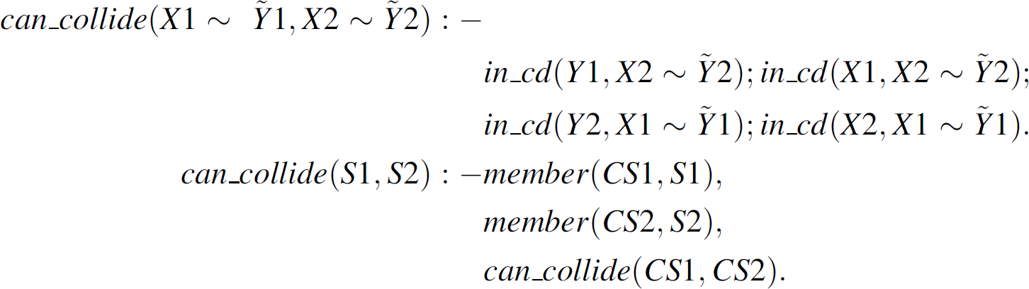
\begin{aligned} t i m e_o v e r l a p (S 1, S 2) : - & s t a r t s (S 1, S T 1), s t a r t s (S 2, S t 2), \\ e n d s (S 1, E T 1), e n d s (S 2, E T 2), \\ ((S T 2 \leq E T 1, E T 2 \geq S T 1); \\ (S T 1 \leq E T 2, E T 1 \geq S T 2)) . \end{aligned}

member(X∼Y, S). This predicate is true if the elementary transmission X∼Y is included in a complex transmission S.

in_cd(X, X1∼Y1). This predicate is true if node X is located in the collision domain of elementary transmission X1∼X2:

i n_c d (X, X 1 \sim \tilde{Y} 1) : - i n_r a n g e (X, X 1); i n_r a n g e (X, Y 1) .

can_collide(S1, S2). This predicate specifies that concurrent execution of transmissions S1 and S2 may result in collisions. The first rule considers the case when both S1 and S2 are elementary transmissions. The second rule deals with complex transmissions.

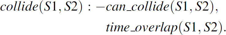
\begin{aligned} c a n_c o l l i d e X 1 \sim \tilde{Y} 1, X 2 \sim \tilde{Y} 2 : - \\ i n_c d (Y 1, X 2 \sim \tilde{Y} 2); i n_c d (X 1, X 2 \sim \tilde{Y} 2); \\ i n_c d (Y 2, X 1 \sim \tilde{Y} 1); i n_c d (X 2, X 1 \sim \tilde{Y} 1) . \\ c a n_c o l l i d e (S 1, S 2) : - & m e m b e r (C S 1, S 1), \\ m e m b e r (C S 2, S 2), \\ c a n_c o l l i d e (C S 1, C S 2) . \end{aligned}

collide(S1, S2). This predicate specifies that concurrent execution of transmissions S1 and S2 results in collisions.

\begin{aligned} c o l l i d e (S 1, S 2) : - & c a n_c o l l i d e (S 1, S 2), \\ t i m e_o v e r l a p (S 1, S 2) . \end{aligned}

5.2. Query Constraints

strict_precede(S1, S2). This predicate states that query semantics require schedule S1 to be executed before schedule S2:

\begin{aligned} s t r i c t_p r e c e d e (S 1, S 2) : - & e n d s (S 1, E T 1), \\ s t a r t s (S 2, S T 2), \\ S T 2 > E T 1. \end{aligned}

precede(S1, S2). This predicate states that schedules S1 and S2 must be executed in an order (either S1 follows S2, or S2 follows S1):

\begin{aligned} p r e c e d e (S 1, S 2) : - & s t r i c t_p r e c e d e (S 1, S 2); \\ s t r i c t_p r e c e d e (S 2, S 1) . \end{aligned}

no_conflict(S1, S2). This predicate states that transmissions S1 and S2 can be executed concurrently without violating any query-imposed orders and without risk of collisions:

\begin{aligned} n o_c o n f l i c t (S 1, S 2) : - & n o t p r e c e d e (S 1, S 2), \\ n o t c a n_c o l l i d e (S 1, S 2) . \end{aligned}

5.3. Validity of DTA Schedules

At this point we are ready to specify semantics of the DTA schedules in terms of the predicates introduced above. First, we should define a mapping of the DTA terms into our semantic domain. We assume an identity mapping function between Node sort of DTA signature and wireless nodes. We also assume that any DTA term X∼Y will map in elementary transmission X∼Y. DTA terms comp(S1,S2), where comp denotes one of the DTA operations o, c, or a will map in the complex transmission that includes all elementary transmissions et_i ∊ subs(comp(S1, S2)). We will represent a data transmission as a list of its elementary transmissions [et₁, …, et_n]. The mapping is defined via the following map predicate:

\begin{aligned} m a p & (X \sim \tilde{Y}, [X \sim \tilde{Y}]) . \\ m a p & (c o m p (S 1, S 2), R e s u l t) : - \\ m a p (S 1, M S 1), m a p (S 2, M S 2), \\ a p p e n d (M S 1, M S 2, R e s u l t) . \end{aligned}

The first map rule specifies that any elementary transmission X∼Y schedule is mapped to an actual data transmission represented as a list [X∼Y] whose only member is the given elementary transmission. The second rule applies the map predicate recursively to the components of a complex schedule and generates the resulting complex transmission as a list of elementary transmissions appending the results of the component mappings. Predicate append(L1,L2,R) is true if list R is a concatenation of the lists L1 and L2.

Example 2. Consider the DTA schedule inferred in Example 1: a(n4 ∼ n2, o(n5∼n3, n3∼n1)). Using the map predicate it will be mapped in the following list of elementary transmissions: [n4∼n2, n5∼n3, n3∼n1].

The following valid predicate specifies semantics for each of the DTA operations:

\begin{aligned} v a l i d (X \sim Y) : - & w i r e l e s s N o d e (X), w i r e l e s s N o d e (Y), \\ r e a c h a b l e (X, Y) . \\ v a l i d (o (S 1, S 2)) : - & v a l i d (S 1), v a l i d (S 2), \\ m a p (S 1, M S 1), m a p (S 2, M S 2), \\ s t r i c t_p r e c e d e (M S 1, M S 2) . \\ v a l i d (c (S 1, S 2)) : - & v a l i d (S 1), v a l i d (S 2), \\ m a p (S 1, M S 1), m a p (S 2, M S 2), \\ p r e c e d e (M S 1, M S 2) . \\ v a l i d (a (S 1, S 2)) : - & v a l i d (S 1), v a l i d (S 2), \\ m a p (S 1, M S 1), m a p (S 2, M S 2), \\ n o_c o n f l i c t (M S 1, M S 2) . \end{aligned}

The definition of the valid predicate consists of four rules with one rule per DTA operation. Elementary transmission X∼Y is valid if the participating wireless nodes X and Y are reachable from each other, i.e., X and Y are in each other's transmission ranges. Strict order o(S1,S2) is valid if both S1 and S2 are valid schedules, S1 is executed before S2 (imposed by strict_precede predicate). The validity of c(S1,S2) and a(S1,S2) is defined using precede and no_conflict predicates.

Using the valid predicate we can define a DTA semantic entailment, or logical implication relation:

Definition 2 (DTA semantic implication). DTA term t is semantically implied by a set of DTA schedules S (denoted $S | = t$ ) if t is valid whenever all t_i ∊ S are valid.

6. Soundness, Completeness and Collisionless of DTA Scheduling

6.1. Soundness

Lemma 1 (can_collide commutativity). can_collide(X,Y) ≡ can_collide(Y,X).

Proof. The proof follows from the definition of can_collide predicate.

Theorem 1 (DTA Soundness). For any set of DTA schedules S and a DTA schedule t, if $S | - t$ then $S | = t$ .

Proof. The soundness of rules 1 and 2 follows from the definition of strict_precede predicate. The soundness of rule 3 follows from the definition of precede predicate. Soundness of rule 4 follows from the commutativity of can_collide predicate (Lemma 1).

Sub-schedule order. First we prove the left sub-schedule order. Consider two valid DTA schedules X and S and assume that there is a sub-schedule S_i ∊ subs(S) such that valid(o(X,S_i)). This implies that there are elementary transmissions et1, et2, and mappings map(S_i,MS_i) such that member(et2,MS_i) and valid(o(et1,et2)). Meanwhile, S_i∊subs(S) also implies member(et2,MS), where map(S, MS). Then, from the definition of strict_precede we conclude valid(o(X,S)). The proof of right sub-schedule order is conducted in the same way.

Sub-schedule choice and Sub-schedule overlap. The structure of the proof has the same schema as the proof of sub-schedule orders. The proof is based on the definitions of the precede and no_conflict predicates.

6.2. Completeness

Generally speaking, the DTA inference rules are not complete, i.e., we cannot prove that for any set of DTA schedules S and a DTA schedule t, if $S | = t$ then $S | - t$ . As an example consider two valid elementary transmissions et1 and et2 such that not precede(et1,et2), and not can_collide(et1,et2). Then ${e t 1, e t 2} | = a (e t 1, e t 2)$ . However, we cannot infer a(et1,et2) from {et1,et2} using the DTA rules. The reason is that DTA does not utilize the low-level semantics of transmission ranges and collision domains. Meanwhile, we can prove that the DTA rules are complete with respect to a given query: if the initial DTA specification reflects basic environment and query constraints, then any valid DTA schedule is also DTA inferable. Below we formally introduce the concept of the query completeness (q-completeness) and prove q-completeness of the DTA inference rules.

Definition 3 (query tree). For a given query Q we define a query tree T_Q as a set of all elementary transmissions required to evaluate Q.

Example 3. Consider query Q from Fig. 2. Then T_Q = {n4∼n2, n2∼n1, n5∼n3, n3∼n1}.

Definition 4 (q-complete set). A set of DTA schedules S_Q is query complete (q-complete) with respect to a query Q if it includes all elementary transmissions of the query tree T_Q and all valid schedules c(eti, etj) and a(eti, etj) over the elementary transmissions of T_Q.

More formally

\begin{aligned} S_{Q} = T_{Q} \cup \\ {c (e t i, e t j) | e t i, e t j \in {T_{Q}}^{\land} v a l i d (a (e t i, e t j))} \cup \\ {a (e t i, e t j) | e t i, e t j \in {T_{Q}}^{\land} v a l i d (c (e t i, e t j))} \end{aligned}

Example 4. For query Q from Fig. 2

\begin{aligned} S_{Q} = & {n 4 \sim \tilde{n} 2, n 2 \sim \tilde{n} 1, n 5 \sim \tilde{n} 3, n 3 \sim \tilde{n} 1, \\ c (n 2 \sim \tilde{n} 1, n 3 \sim \tilde{n} 1), \\ a (n 4 \sim \tilde{n} 2, n 5 \sim \tilde{n} 3), a (n 4 \sim \tilde{n} 2, n 3 \sim \tilde{n} l), \\ a (n 5 \sim \tilde{n} 3, n 2 \sim \tilde{n} 1)} \end{aligned}

Theorem 2 (DTA q-completeness). For any query Q and a DTA schedule t, if $S_{Q} | = t$ then $S_{Q} | - t$ .

Proof. Assume that $S_{Q} | = t$ , but not $S_{Q} | - t$ . If t is the elementary transmission or comp(S1,S2), where comp is either c or a and S1, S2 are elementary transmissions, then by definition of $S_{Q} : S_{Q} | = t \Rightarrow t \in S_{Q} \Rightarrow S_{Q} | - t$ t. If t is a o(S1,S2), where S1 and S2 are elementary transmissions, then t can be inferred from S_Q by finite number of applications of the DTA rules 1 (order introduction) and 2 (order transitivity). If t is a o(S1,S2) and at least one of S1 or S2 is not an elementary transmission, then t can be inferred from S_Q by finite number of applications of the DTA sub-schedule rules 2, 5, and 6. If t is a comp(S1,S2), where comp is either c or a and at least one of S1 or S2 is not an elementary transmission, then t can be inferred from S_Q by finite number of applications of the DTA rules 3, 4, 7, and 8. Thus, $S_{Q} | = t$ implies $S_{Q} | - t$ □

6.3. Derived DTA Rules, Executable Schedules and Deadlocks

In order to increase the performance of our algebraic optimization we use the basic DTA rules to infer a set of derived rules. Figure 6 shows some examples of the derived DTA rules. The derived rules are utilized by our randomized optimizer as valid moves between DTA schedules [12, 29, 31].

Figure 6.

Derived DTA Inference Rules.

It is interesting to note that the expected order associativity o(o(X,Y),Z) ↔ o(X,o(Y,Z)) and the choice associativity c(c(X,Y),Z) ↔ c(X,c(Y,Z)) are not sound inference rules. Consider a query tree in Fig. 7. The following DTA schedule is valid: o(o(a(n1∼n5,n4∼n8), n9∼n11), n10∼n12). However, the schedule o(a(n1∼n5,n4∼n8),o(n9∼n11, n10∼n12)) is not valid, since valid(o(n9∼n11, n10∼n12)) is not true. Similarly, c(c(n7∼n10,n8∼n10), n6∼n9) is valid, while c(n7∼n10, c(n8∼n10, n6∼n9)) is not valid. With the tree topology of Fig. 7 transmissions n8∼n10 and n6∼n9 can be executed concurrently, i.e., valid(a(n8∼n10, n6∼n9)) holds.

Figure 7.

Invalidation of order and choice associativity.

It should be noted that while being invalid the above schedules o(n9∼n11, n10∼n12) and c(n8∼n10, n6∼n9) are still executable. Indeed, the fact that query semantics do not impose a strict order on the transmissions n9∼n11 and n10∼n12 does not mean that we cannot execute them in the order o(n9∼n11, n10∼n12). The same is true about n8∼n10 and n6∼n9. An interesting question is if it is possible to generate a valid DTA schedulec which would not be executable. This question has a positive answer. An example of a valid non-executable schedule is a deadlocked schedule.

Definition 5 (deadlock-potential schedules). DTA schedules S1 and S2 are deadlock-potential if both o(S1,S2) and o(S2,S1) are valid.

For example, in the query tree in Fig. 7 schedules a(n1∼n5, n10∼n12) and a(n4∼n8, n9∼n11) are deadlock-potential. This is implied by the fact that both o(n1∼n5, n9∼n11) and o(n1∼n5, n9∼n11) are valid. Then, a strict order of the deadlock-potential schedules will make a valid non-executable deadlocked schedule. The following is an example of a valid deadlocked schedule:

o (a (n 1 \sim \tilde{n} 5, n 10 \sim \tilde{n} 12), a (n 4 \sim \tilde{n} 8, n 9 \sim \tilde{n} 11)) .

In order to capture the deadlock semantics we extend the DTA semantic definition from Section 5 with deadlock(T1,T2) predicate stating that DTA transmissions T1 and T2 are deadlocked. The following rule provides a formal definition of the deadlock predicate:

\begin{aligned} d e a d l o c k (T 1, T 2) : - & s t r i c t_p r e c e d e (T 1, T 2), \\ s t r i c t_p r e c e d e (T 2, T 1) . \end{aligned}

Note, that negation of the deadlock predicate in the body of the valid(o(S1,S2)) rule (Section 5) would invalidate the deadlocked schedules. This, however, would add more complexity to DTA inference rules in order to maintain DTA soundness and completeness. In order to preserve reasonable complexity of the query optimization we allow DTA rules to generate deadlocked schedules. Instead of making DTA deadlock-free we implemented efficient deadlock handling strategies with further consideration of which is out of scope of this paper.

6.4. Collision-free DTA Schedules

Finally, we prove a key property of DTA: DTA inference rules generate only collision-free schedules.

Definition 6 (collision-free schedule). A DTA schedule S is collision-free if ∀S_i, S_j ∊ subs(S), Si ≠ Sj, map(Si, Ti), map(Sj, Tj) impliesnotcollide(Ti, Tj).

Theorem 3 (valid schedule is collision free). For any DTA schedule t, if valid(t) then t is collision free.

Proof. If t is an elementary transmission then the fact that t is collision-free follows from Definition 5. Indeed, in this case ∀S_i, S_j ∊ subs(t)S_i = S_j = t. Suppose t is a composed schedule comp(S1,S2), where comp is either o or c. Since t is valid, then there are mappings map(S1,T1) and map(S2,T2) such that time_overlap(T1,T2) is false (this follows from the definition of strict_procede and procede predicates). Thus, collide (T1,T2) is false, which implies that t is collision-free. Now assume that t is a composed schedule a(S1,S2). Since t is valid, then there are mappings map(S1,T1) and map(S2,T2) such that can_collide(T1,T2) is false (this follows from the definition of no_conflict predicates). Thus, collide(T1,T2) is false, which implies that t is collision-free.

Corollary 1 (DTA-inferable schedule is collision free). For any set of valid DTA schedules S and a DTA schedule t, if $S | - t$ then t is collision free.

Proof. The proof follows from soundness of DTA (Theorem 1) and Theorem 3.

7. Implementation of the DTA-based Optimizer

We implemented a cost-based multi-objective query optimizer that identifies DTA schedules with an acceptable query response time and overall energy consumption. In general, a multi-objective optimization (MOP) aims at minimizing values of several objective functions f1,…fn under a given set of constraints. In most cases it is unlikely that different objectives would be optimized by the same parameter choice. Informally, an objective vector is Pareto optimal [17] if all other feasible vectors in the objective space have a higher value for at least one of the objective functions, or else have the same value for all objectives. For example, if the following set includes feasible solutions for biobjective MOP: {(5,1), (2,2), (2,3), (1,5)}, then the Pareto optimal set (also called Pareto front) is {(5,1), (2,2), (1,5)}.

Among all Pareto optimal solutions, our optimizer chooses one using an application-dependent utility function. The optimizer evaluates time and energy gains/losses, and makes a preference considering the relative importance of time and energy in the context of a specific query. Figure 8 presents the algorithm that our optimizer uses to compute time/energy utility function. The algorithm inputs two Pareto optimal objective vectors (T1,E1) and (T2,E2), where T1, T2 are response times and E1,E2 - consumed energy; in addition the optimizer considers two factors: time factor TF and energy factor EF ranging from 0 to 1. The higher the TF (EF), the more importance the optimizer gives to the time (energy) savings. Consider the Pareto set from a previous subsection: {(5,1), (2,2), (1,5)}. Then UF((5,1),(2,2),0.8,0.2) will return (5,1), while UF((5,1),(2,2),0.2,0.8) results in (2,2). In general UF impose an order on the Pareto set for a given setting of TF and EF. For example, with TF = 0.2 and EF = 0.8 the order would be {(2,2),(1,5),(5,1)}.

Figure 8.

Calculating Time/Energy utility function.

DTA scheduling may be expensive due to its combinatorial nature. The number of alternative schedules grows exponentially with the number of sensor nodes and elementary transmissions participating in a query. In general, for a query tree with n (n > 1) elementary transmissions the total number of all possible complete DTA schedules involving those transmissions will be equal to a number of permutations of n transmissions without repetitions multiplied by a number of total variations of three DTA operations with repetitions of length (n - 1):

N u m_o f D T A_s c h e d u l e s (n) = n! \times 3^{(n - 1)}

For example of the two elementary transmissions t1 and t2 we can generate 2! × 3⁽²⁻¹⁾ = 6 schedules, namely: o(t1,t2), o(t2,t1), c(t1,t2), c(t2,t1), a(t1,t2), a(t2,t1).

In order to cope with the expected scheduling complexity our optimizer utilizes randomized algorithms [12] to generate Pareto fronts for larger query trees. Randomized algorithms search for a solution of a combinatorial problem in a large space of all possible solutions. Each solution is associated with application-specific cost. Randomized algorithms are searching for a solution with the minimal cost performing random walks in the solution space via series of valid moves. In our case possible solutions are DTA schedules. Specific algorithms are different with respect to moving strategies and stopping conditions. We explore the performance of each of them for the purpose of scalable DTA scheduling. Figure 9 illustrates how DTA scheduling utilizes Iterative Improvement algorithm. Variables and parameters of the algorithm are explained in Table 1. Initially the II algorithm assigns a serial schedule Sser that performs all elementary transmissions sequentially as an optimal schedule minS. Then it tries to improve this serial baseline increasing the concurrency benefit of the initial schedule. Concurrency benefit is a part of the time cost that can be “hidden” by scheduling some transmissions concurrently. A more accurate definition of the concurrency benefit is presented in section 8, where we provide an experimental evaluation of our optimizer. Valid moves between DTA schedules correspond to valid DTA transformations introduced in Sections 4 and 6.

Figure 9.

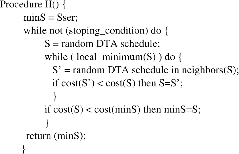
II Optimization Algorithm for DTA scheduling.

Table 1

Explanation of Variables and Parameters of II Algorithm

minS	Current DTA schedule with minimal cost
Sser	Random serial DTA schedule
S	Random initial DTA schedule
neighbors(S)	Set of schedules that can be generated from S via one valid move
stopping_condition	Number of considered initial schedules
local_minimum(S)	Number of neighbors of S to be tested, of which none has lower cost than S. If the test id successful, S is considered to be a local minimum

The optimizer utilizes a cost model that associates execution time and energy consumption with each DTA schedule. For example, the execution time of elementary transmission ni∼nj consists of local processing times Tp at nodes ni and nj plus the time Ttx required for transmitting data from ni to nj. The execution time of a strict order of schedules A and B is the sum of the execution times of A and B. For concurrent schedules A and B, the execution time would be the maximum of the execution times of A and B. The energy model is for elementary transmission and is based on a path-loss equation. The energy cost model for elementary transmission is based on a path-loss equation that approximates the power loss with distance [28]. For complex schedules the energy cost is a sum of energy costs for each elementary transmission involved in that schedule. More details on the optimizer cost modeling are provided in [28, 29].

In order to support DTA query scheduling the optimizer should rely upon highly available and accurate query statistics and other relevant network meta-data including current network topology, processing and transmission delays, collision domains, and current distribution of pre-aggregated and materialized data. Part of such query statistics and network meta-data should be reflected in an initial DTA specification and it should be stored in a highly available distributed repository with varying freshness, precision, and availability requirements. Design and implementation of such a repository together with an appropriate signaling system is a considerable challenge. Currently our optimizer utilizes a centralized scheme for the implementation of such a meta-data repository, where all the statistics metadata is maintained in a central node accessible through a base station. In a centralized scheme, the root node is a base station (BS) with a large broadcast area and unlimited power supply since it is presumably a fixed node and located in an opportunistic location. The BS maintains the statistics on processing and transmission delays, the network topology, and collision domains. The synchronization of the participating nodes can be easily achieved, since every node listens to the same BS. The BS performs query scheduling using DTA and broadcasts the resulting schedule to every node in the network. For this purpose, out-of-band signaling or periodic beacons can be employed.

We also explore more distributed schema, where each wireless node maintains statistics meta-data about itself. A query can be submitted at a root node of a routing tree and then propagates down the tree to every node. After receiving a query, each child node in the lowest level provides its statistics, i.e., processing and transmission times (delays) to their parent. Then, the parent node performs query scheduling for each child node using DTA in order to minimize collisions and the active time for the parent's receiver. The parent node returns this schedule to its children. After scheduling its children, the parent node estimates and sends its own processing and transmission delay information to an upper level parent node. Then the same process propagates up the routing tree until it reaches the root node. The above process can vary depending on actual query and network statistics. For example, the transmission time of the latest node can be fixed and the transmissions for the remaining nodes should be scheduled ahead of the latest node. Under a different scheme, every node in the sensor network is associated with its own statistics metadata, and some of the nodes can additionally host statistics meta-data (perhaps more summarized) about a subnet of devices in their local meta-data repository.

An algebraic optimization as explained above assumes that the sensor nodes are stationary. Meanwhile, we can also apply the DTA-optimizer to improve the performance of Mobile Sensor Networks (MSNs). In MSNs wireless sensor devices can be attached to mobile devices such as mobile robots. Mobile sensors platform can be deployed in conjunction with stationary sensor nodes to acquire and process data for surveillance and tracking, environmental monitoring for highly sensitive areas, or execute search and rescue operations. Resource constraints of MSNs make it difficult to utilize them for advanced environmental monitoring that requires data intensive collaboration between the nodes (e.g., exchange of multimedia data streams). In general, the time/energy tradeoffs involve energy and time gains/losses associated with specific layouts of the nodes. Both relocation and changing the transmission range of sensor nodes could result in changing the number of potential collision-free concurrent transmissions. Those factors can also result in changing the number of hops and intermediate transmission nodes involved in query execution. This, however, brings both benefits and penalties. If the filtering factor of the intermediate node is low (i.e., it just retransmits the data) then introducing it we expect to have some time and energy loss due to extra hop. From the other side the intermediate node does reduce the data transmission ranges, which results in saving some energy. If the intermediate node does a lot of filtering, the benefit includes spending less energy in order to transmit less data.

An algebraic query optimization based on DTA can be used to generate query routing trees to maximize collisionless concurrent data transmissions taking into account intermediate hops and filtering factors of mobile facilitators. Figure 10 shows a query tree topology with four previously positioned nodes s0, s1, s2, s3 and three different positions of a mobile facilitator m. The facilitators consume extra energy and introduce some extra processing delay. However, by reducing the transmission range and data stream sizes, they are also capable of reducing the overall query time and energy consumption. Note, how the re-positioning of the facilitator is reflected in the initial DTA specifications is1, is2 and is3.

Figure 10.

Impact of mobility on DTA specification.

Out of the many possible query routing trees and transmission schedules the optimizer should select an option with an acceptable query response time and overall energy consumption. Further details on the implementation of our optimizer are in [28, 29].

8. Experimental Evaluation of the DTA-based Optimizer

First we report on the behavior of the DTA scheduler for a medium complexity query tree involving ten sensor nodes with conflicting collision domains. Figure 11 represents some of our preliminary experimental graphs characterizing the performance of II algorithm. Processing and transmission costs were generated randomly using Gaussian distributions. As a baseline, we consider a serial scheduling strategy that performs elementary transmissions sequentially. Figure 11 reports on time costs and concurrency benefits of selected schedules. Recall from section 7 that the concurrency benefit is a part of the time cost that the DTA scheduler is able to “hide” scheduling some transmissions concurrently. The benefit is defined recursively for each of the DTA operations. The benefit of a(X,Y) is equal to minimum of costs cost(X) and cost(Y). For the rest of the DTA operations the benefit is equal to zero. Thus, any serial schedule has a zero benefit. In addition to costs and benefits of serial and winner schedules we also report a value of gain received from the local minimum phase of the algorithm. We observe that the performance of the II algorithm consistently improves as we increase the stopping condition and the local minimum conditions.

Figure 11.

Performance of II algorithm.

Figure 12 reports on Pareto fronts explored by the optimizer for a two-hop query tree of 8 nodes with some data aggregation/filtering at intermediate nodes. For example, filtering factor 0.2 means that 20% of data delivered to an intermediate node will be forwarded to the base station. A major observation here is an increase of variability in both time and energy consumption with a decrease of the facilitator filtering factor. For the filtering factor of 0.2 the energy varies between 66000 mJ and 80000 mJ, while for the filtering factor of 0.8 the energy range is 78000–81000 mJ. The time ranges are 46–76 sec and 64–95 sec correspondingly. The optimizer should explore related time/energy tradeoffs maximizing benefits and avoiding risks of selecting bad schedules.

Figure 12.

Actual Pareto fronts explored by optimizer.

Figure 13 shows the optimization choices for one of the generated Pareto fronts using the utility function described in Fig. 8. The choices are made for different time and energy factors. We observe a consistent optimizer behavior in making preferences with respect to the time and energy factors. We observed similar performance trends with other query tree topologies considered in our experiment.

Figure 13.

Effect of TF and EF on utility-based tree selection.

Figure 14 reports on the packet success ratio representing the percentage of transmitted packets that reach a destination (sink) node successfully. Recall, that it was a low packet success ratio that caused network collapses for higher traffic loads from critical monitoring applications, so it is important to observe how DTA helps to maintain it compared to the typical IEEE 802.15.4 that uses carrier sense multiple access with collision avoidance (CSMA-CA) [33]. We experimented with medium and large starlike networks using CMU wireless and mobility extensions to ns-2 simulator [20]. The medium network consists of 25 nodes positioned within a 150 × 150 meters flat area while the medium network includes 73 nodes. All nodes (except the central sink node) deliver packets to the sink in multi-hop fashion. We used 250 Kbps channel data rate with the sensor transmission range of 15 meters.

Figure 14.

Packet success ratio for medium and large networks.

Figure 14 (left graph) shows the simulation results for a medium network. We observe that at lower loads, the packet success ratio of DTA is around 98%. It decreases to 80% as the data generation rate increases to 40 packets/second. This slight degradation is caused by an insufficient queue buffer size of the sensor nodes. Meanwhile, even at very low traffic loads (0.5 and 1 packet/sec) CSMA delivers only 70% of data to the sink node. When the load increases, the CSMA network becomes overloaded with collided or lost packets and the packet success ratio drops to 30%.

The benefit of DTA becomes even more obvious for a large network (Fig. 14, right graph). At lower rates, the DTA packet success ratio is around 95%. The ratio decreases to 40% as the data generation rate increases to 27 packets/second. This is because the traffic load exceeds the channel data rate (250 Kbps). Meanwhile, the packet success ratio with CSMA drops to less then 20% almost immediately.

9. Conclusion

A major contribution of this paper is a formal discussion of algebraic query scheduling in sensor networks. Such scheduling is one of the key elements for improving the performance of queries with respect to both the response time and the energy consumption. Specifically, we introduced and formally characterized a Data Transmission Algebra (DTA) that utilizes the information about how the lower network layers operate while processing queries in sensor databases. Our DTA uniformly captures the constraints of data transmissions and provides a background for novel cross-layer query optimization. Using the DTA, an optimizer can perform collision-aware query scheduling that avoids simultaneous interfering transmission. We considered DTA soundness and completeness and proved that DTA inference rules generate only collision-free transmission schedules. We described and evaluated a DTA-based query optimizer that performs collision-aware query scheduling.

Footnotes

Acknowledgments

We would like to thank Prashant Krishnamurthy for his valuable feedback and Chih-Kuang Lin for his help with the experiments.

References

Bonnet

Gehrke

, and Seshadri

. “Towards sensor database systems”, in Proceedings of MDM Conference, 2001.

Bonnet

and Seshadri

. “Device database systems,” in Proceedings of ICDE Conference, 2000.

Beaver

Sharaf

M. A.

Labrinidis

, and Chrysanthis

P. K.

, “Location-aware routing for data aggregation in sensor Networks,” in Proceedings of the 2nd Hellenic Data Management Symposium, 2003.

Cetintemel

Flinders

, and Sun

, “Power-efficient data dissemination in wireless sensor networks”, in Proceedings of ACM MobiDE Workshop, 2003.

Considine

Kollios

and Byers

, “Approximate aggregation techniques for sensor databases,” in Proceedings of IEEE ICDE Conf., 2004.

Crow

Widjaja

Kim

L.G.

Sakai

P.T.

. “IEEE 802.11 Wireless local area networks,” IEEE Communications Magazine, vol. 35, no. 9, pp. 116–126, Sept. 1997.

Despande

Guestrin

Madden

Hellerstein

Hong

, “Model-driven data acquisition in sensor networks,” in Proceedings of VLDBConf., 2004.

Ehrig

Mahr

, Fundamentals of Algebraic Specification. Equations and Initial Semantics. Springer-Verlag, 1990.

Farrar

Doebling

S. W.

Nix

D. A.

, “Vibration-based structural damage identification,” Philosophical Transactions of the Royal Society of London: A – Mathematical, Physical, and Engineering Sciences, 2001.

10.

Goel

and Imielinski

, “Prediction-based monitoring in sensor networks: Taking lessons from MPEG,” Computer Comm. Review, vol. 31, no. 5, 2001.

11.

Grant

Zadorozhny

, “Logical approach to capability-based rewriting in a mediator for websources,” Journal of Intelligent Information Systems (JIIS), vol. 17, no. 1, 2001.

12.

Ioannidis

Y. E.

Kang

, “Randomized algorithms for optimizing large join queries,” ACM SIGMOD, 1990.

13.

Jones

C. E.

Sivalingam

K. M.

Agrawal

, and Chen

J. C.

, “A survey of energy efficient network protocols for wireless networks,” Wireless Networks, vol. 7, 2001.

14.

Heidemann

Silva

Intanagonwiwat

Govindan

Estrin

and Ganesan

, “Building efficient wireless sensor networks with low-level naming,” in Proceedings of ACM SOSP, 2001.

15.

Heinzelman

W. R.

Chandrakasan

, and Balakrishnan

, “Energy-efficient communication protocol for wirelessmicrosensor networks,” in Proceedings of HICSS Conf., 2000.

16.

Lin

C-K.

Sharma

Zadorozhny

Krishnamurthy

, “Efficient data delivery in wireless sensor networks: algebraic cross-layer optimization versus CSMA/CA,” Tech. Rep., University of Pittsburgh, 2005.

17.

Miettinen

, Nonlinear Multiobjective Optimization Kluwer Academic Publisher, 1999.

18.

Madden

Franklin

M. J.

Hellerstein

J. M.

, and Hong

, “Tag: A tiny aggregation service for ad hoc sensor networks,” in Proceedings of OSDI, 2002.

19.

Madden

Franklin

M. J.

Hellerstein

J. M.

, and Hong

, “Tag: the design of an acquisitional query processor for sensor networks,” SIGMOD 2003.

20.

The CMU Monarch Project's Wireless and Mobility Extensions to NS, http://www.monarch.cs.cmu.edu/cmu-ns.html.

21.

Pahlavan

and Levesque

, Wireless Information Networks, John Wiley and Sons, 1995.

22.

Pahlavan

and Krishnamurthy

, Principles of Wireless Networks: A Unified Approach, Prentice Hall, 2002.

23.

Sharaf

M. A.

Beaver

Labrinidis

, and Chrysanthis

P. K.

, “TiNA: A scheme for temporal coherency-aware in-network aggregation,” in Proceedings, of ACM MobiDE Workshop, 2003.

24.

Sharma

Zadorozhny

V. I.

Chrysanthis

P. K.

, “Structural health monitoring with whirlpool,” in Proceedings of 5th Int. Workshop on Structural Health Monitoring, 2005.

25.

Rangwala

Chintalapudi

Ganesan

Broad

Govindan

Estrin

., “A wireless sensor network for structural monitoring,” in Proceedings of SenSys, 2004.

26.

Yao

and Gehrke

J. E.

. “The cougar approach to in-network query processing in sensor networks,” SIGMOD Record, vol. 31, no. 3, 2002.

27.

Younis

Youssef

and Arisha

., “Energy-aware routing in cluster-based sensor networks,” in Proceedings of MASCOTS, 2002.

28.

Zadorozhny

Sharma

Krishnamurthi

Labrinidis ., “A Tuning query performance in mobile sensor databases,” in Proceedings of the 6th International Conference on Mobile Data Management (MDM), 2005.

29.

Zadorozhny

V. I.

Chrysanthis

P. K.

Krishnamurthy

, “A framework for extending the synergy between MAC layer and query optimization in sensor networks,” in Proceedings of DMSN VLDB Workshop, 2004.

30.

Zadorozhny

V. I.

Chrysanthis

P. K.

Labrinidis

, “Algebraic optimization of data delivery patterns in mobile sensor networks,” in Proceedings of MDDS DEXA Workshop, 2004.

31.

Zadorozhny

V. I.

Raschid

Vidal

M. E.

Urhan

and Bright

, “Efficient evaluation of queries in a mediator for websources,” in Proceedings of ACM SIGMOD, 2002.

32.

Zadorozhny

V. I.

Chrysanthis

P. K.

, “Location-Based Computing,” in Telegeoinformatics: Location-Based Computing and Services, Taylor and Francis Inc., 2003.

33.

Zheng

and Lee

M. J.

, “Will IEEE 802.15.4 make ubiquitous networking a reality? A discussion on a potential low power, low bit rate std. IEEE Communications Magazine, June 2004.

Sensor Queries: Algebraic Optimization for Time and Energy

Abstract

Keywords

1. Introduction

2. System Model

5. DTA Semantics

5.1. Environment Constraints

5.2. Query Constraints

5.3. Validity of DTA Schedules

6. Soundness, Completeness and Collisionless of DTA Scheduling

6.1. Soundness

6.2. Completeness

6.3. Derived DTA Rules, Executable Schedules and Deadlocks

7. Implementation of the DTA-based Optimizer

Footnotes

Acknowledgments

References