
Abstract
This paper solves the problem of estimation of the parameters of a hyperexponential density and presents a practical application of the solution in sensor networks. Two novel algorithms for estimating the parameters of the density are formulated. In the first algorithm, an objective function is constructed as a function of the unknown component means and an estimate of the cumulative distribution function (cdf) of the hyperexponential density. The component means are obtained by minimizing this objective function, using quasi-Newtonian techniques. The mixing probabilities are then computed using these known means and linear least squares analysis. In the second algorithm, an objective function of the unknown component means, mixing probabilities, and an estimate of the cdf is constructed. All the 2M parameters are computed by minimizing this objective function, using quasi-Newtonian techniques. The developed algorithms are also compared to the basic EM algorithm, and their relative advantages over the EM algorithm are discussed. The algorithms developed are computationally efficient and easily implemented, and hence, are suitable for low-power and sensor nodes with limited storage and computational capacity. In particular, we demonstrate how the structure of these algorithms may be exploited to be effectively utilized in practical situations, and are hence ideal for sensor networks.
Keywords
Introduction
The advent of sensor networks has spurred research to develop new methods for distributed data collection and processing. Estimation of parameters of physical quantities from data collected over a geographic area is one such task. Mixture density is a powerful family of probability density functions and is useful in representing some physical quantities for such an application. The vast majority of the literature on the subject of mixture densities pertains to Gaussian mixture models (GMM). By comparison, mixtures of exponentials have received far less attention. Notwithstanding, mixtures of exponentials have significant applicability in a number of fields, including computer networks, biology, engineering, and medicine. The class of general mixtures of exponential distributions has relevance in linear systems theory and differential equations (Chauveau [1]). Cao et al [2] discuss modeling of rainfall and contract valuation with hyperexponential densities. Specifically, in the paper by Cao et al [2], the amount of rainfall in an area is modeled using a mixture of two exponential densities. A further exposition of generalized hyperexponential distribution functions may also be found in Botta et al [3]. The focus of this paper is on a subset of exponential probability densities, which will be henceforth referred to as hyperexponential densities. We develop two algorithms for estimating the parameters of hyperexponential densities. The strength of these algorithms lies in the fact that the methods presented require little computational power and that the computations can be decomposed efficiently. These features enable an effective solution that is appropriate for sensor networks as outlined in section I-A.
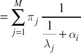
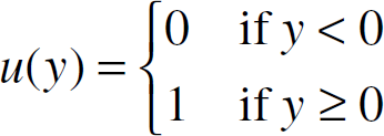
The probability distribution function (pdf) of an M-component hyperexponential density is

where the mixing proportions are given by
We now introduce applications in a sensor network environment, which can be modeled accurately by hyperexponential densities. Sensor networks (Akyildiz et al [4] and Rentala et al [5]) consist of many sensor nodes arranged in either an ordered or random fashion. Figure 1 shows such a sensor network. Data is transmitted via a multi-hop approach from the sensor nodes to special nodes called base stations. Sensor nodes are ideal for sensing environmental changes, especially in hostile or remote locations or over large geographical areas. One important category of environmental observation is rainfall observation in forestry and agriculture. The relevance of the statistical properties of rainfall is expounded in Hansen and Ines [6]. In particular, the quantity of rainfall in an area is decidedly important due to its effect on processes in nature, such as, solute leaching, soil erosion, and crop water stress response. Long-tailed distributions as discussed in the previous sections are useful for modeling the amount of rainfall in an area. Moreover, the amount of rainfall is commonly modeled as a two-component hyperexponential density with pdf

where α, β1 and β2 are estimated parameters ([2] and [6]).
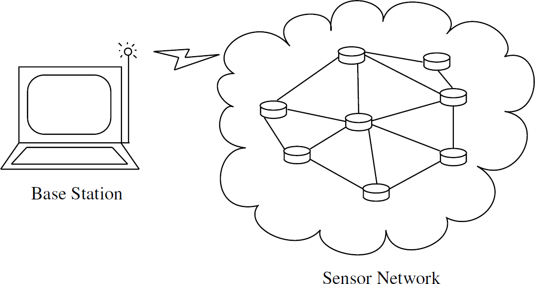
Sensor network.
Sensor nodes fitted with soil moisture sensors are ideal for measuring rainfall and collecting data that would allow for statistical modeling of rainfall. In large, remote, forested areas or large agricultural fields or both, sensor networks would be valuable for collecting rainfall data. Typically, many sensor nodes are scattered or positioned over a large area and these nodes function until their batteries are expended. Due to the limited battery supply in each sensor node, transmissions by sensor nodes should be kept to a minimum. Furthermore, each sensor node has a relatively meager amount of memory (usually about 4K) and processing ability. Therefore, it is also desirable to reduce the complexity of calculations performed by a sensor node.
In the following sections, we develop algorithms for estimating the parameters of a hyperexponential density, which can also be used to obtain the parameters of equation 2 in our rainfall example. The algorithms are also designed so as to work well in a sensor network environment with energy and computational power constraints. That is to say, the data communication and computational power requirements of the sensor nodes are very minimal. In the following subsection, additional motivation for studying hyperexponential densities is presented, as we look at applications in modeling long-tailed distributions.
In recent years, the volume of traffic on large-scaled networks and across the Internet has increased tremendously, necessitating serviceable statistical models for traffic flow and analysis. Statistical models are required for the design of underlying IP-based transport layer protocols, efficient data gathering and evaluation, and statistical analysis of corresponding random processes and variables (Markovitch and Krieger [7]). The work of Leland et al [8] demonstrates that both LANs and WANs exhibit long range dependencies, and hence, classical Poisson-based methods are insufficient for such large-scale networks. Typical Poisson methods predict early fluctuations in network traffic and hinge on the assumption that these anomalies will smooth out over a long period of time. In reality, these fluctuations occur over a wide range of time scales generating high variability and self-similar behavior (Schwefel [9]). The notion of self-similarity and fractal geometry was introduced by Mandelbrot [10] to describe naturally occurring processes using mathematical formulae. Self-similar processes are structurally similar over many different time scales. This phenomenon leads to long range dependencies in network traffic. Indeed, the concept of self-similarity and long range dependencies go hand-in-hand.
Ostensibly, an alternative to classical Poisson methods is sought. To this end, long-tailed distributions have shown much success. A distribution is a long-tailed distribution (also referred to as a heavy-tailed distribution) if its complementary cumulative distribution function (ccdf), Fc, decays slower than exponentially, i.e. if

for all α > 0 (Feldmann and Whitt [11]). The ccdf is defined as the complement of the cumulative distribution function (cdf), as follows

where F(x) is the cdf. Conversely, a distribution is a short-tailed distribution if its ccdf decays exponentially, i.e. if

for some α > 0. Of note is a special case of long-tailed distributions called the power-tail distribution. A distribution is said to be power-tail distribution if

where α and β are positive constants and the operator ∼ is defined such that f(x) ∼ g(x) implies that

Two common examples of long-tailed distributions that are used widely in network performance analysis are the Pareto and Weibull distributions. In addition, the Pareto distribution is a power-tailed distribution; however, the Weibull distribution is not.
Recent studies have demonstrated that long-tailed distributions model many network characteristics aptly. For example, long-tailed distributions have been valuable in modeling World Wide Web (WWW) traffic, since the said traffic often originates from heterogeneous sources [7]. Long-tailed distributions have also been shown to be successful in modeling file transfer protocol (FTP) connections and intervals between connection requests [11]. As effective as the long-tailed distribution has been in capturing the statistical characteristics of large scale networks, there are some deficiencies of this model. Most notably, long-tailed distributions are generally very difficult to analyze. An example is the task of analyzing the performance figures of the basic M/G/1 queue which becomes quite involved if the service-time distribution is Pareto. Furthermore, unlike many short-tailed distributions, expressions for the Laplace transforms of long-tailed distributions are quite complex. Laplace transforms are generally useful for analyzing the distributions by numerical transform inversion. Standard non-parametric estimators such as the histogram, projections, and kernel estimators are not suitable for long-tailed distributions and often exhibit poor estimates or “spikes” in the tail region. It is well-known that kernel estimators suffer from spurious noise appearing in the tail of the estimator [12]. Markovitch and Krieger [7] have explored some non-parametric procedures for estimating and approximating long-tailed distributions. Two of these procedures include transformation functions that map a long-tailed density into a pdf with compact support, and polygrams. Polygrams are histograms with variable bin widths.
The aforementioned problems associated with long-tailed distributions do not appear in short-tailed distributions. Accordingly, a natural proposal for alleviating the problems of long-tailed distributions is to approximate the said long-tailed distributions with corresponding short-tailed distributions. This is justifiable by the fact that although long-tailed distributions do not have compact support, for practical purposes there is only a finite interval for which the distribution in question takes on meaningful values. Therefore, one approach for approximating long-tailed distributions is to effectively truncate the long-tailed distribution, confining it to a finite interval. Intuitively, this method encompasses the essential features of the long-tailed distribution. In spite of this, the truncation approach may not be a suitable technique since the resulting function has discontinuities for values in the real, positive domain. An alternative to approximating the long-tailed distributions by truncating is to use hyperexponential densities. Hyperexponential densities have exhibited much success in approximating long-tailed distributions and for constructing network performance models ([11] and [7]). Moreover, the analysis of hyperexponential densities is tractable and the Laplace transforms are simple expressions.
Two computationally efficient, tractable, and easily implemented algorithm for estimating the parameters of a hyperexponential density are developed and tested. The first algorithm — hereafter, referred to as Algorithm 1 — is a two-step procedure. The first step involves estimating the component rates γ of the hyperexponential distribution. The approach here is to develop equations that express π in terms of γ. These expressions are then substituted into an objective function which is a function of γ and an estimate for the cdf of the hyperexponential distribution. Minimizing this objective function yields the required estimates of λ. The second step estimates the steady state probabilities π given that the component means are known by making use of linear least squares analysis. The second algorithm — Algorithm 2 — estimates π and λ in one phase by minimizing an objective function that is a function of π, λ and an estimate for the cdf of the hyperexponential distribution. The relative merits of each algorithm are also compared and discussed.
Our algorithms are also compared to maximum-likelihood techniques and the expectation-maximization (EM) algorithm (Dempster et al [13]), in particular. Finally, we demonstrate how our algorithms are adapted to work well in a sensor network environment.
Algorithm 1
Most ML techniques for computing the parameters of hyperexponential densities intrinsically require estimation of 2M parameters. Likewise, any optimization procedure that uses or evaluates the hyperexponential density directly, also involves the estimation of 2M parameters. In this section, equations expressing π in terms of λ and functions of the samples of data are derived, thus reducing the number of unknown parameters to M. Making use of these equations, an objective function is formulated and the values of λ are calculated by minimizing this objective function. It is assumed that each mixing proportion is strictly positive, ensuring that each component plays a role in influencing the resulting pdf. Algorithm 1 essentially reduces the number of unknown parameters by incorporating additional information from the structure of the mixture pdf and from samples of data.
Expressions for π
Nonlinear transforms are employed in order to reduce the number of unknown parameters. Specifically, the Laplace transform of the exponential density is exploited. Define

Let A be the matrix with elements


provided that

at row i and column j and where λ1 ≠ λ2 ≠ … ≠ λ
M
≠ 0 and α1 ≠ α2≠ … ≠ α
M
. Clearly, each λ
i
is distinct by the assumption that the mixing proportions for each component are all non-zero, and each α
i
is distinct by assumption. Hence, A is clearly invertible. From equations (11) and (12) the steady state probabilities may be expressed as

This gives a means of computing π if the component means and expectations in equation (9) are provided.
The expressions for the mixing probabilities developed in the previous section afford a means of reducing the number of unknown variables to just M. In this section, an algorithm to obtain this M component mean vector is formulated by fitting a candidate cdf to the given exact cdf. The approach iteratively attempts to improve the fit of a real or estimated cdf to that of a cdf constructed from successive approximations of the parameter set. The cdf of a hyperexponential density is

Let
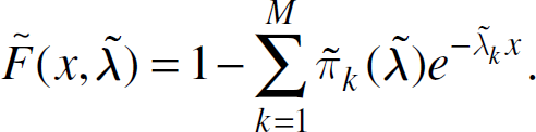
Notice that the only unknown in this candidate cdf is

This result can be extended over the entire domain of x — i.e. the set of all real numbers greater than or equal to zero (

Observe that


In order to minimize the objective function developed, there are several quantities that need to be estimated from the samples of data. In this section, estimators for these quantities are devised. Given n samples of data w = {w1… .,wn}, and assumed distinct constants α
i
, an estimator for ai is

Define â to be the estimate of a from the samples of data.
The equations derived previously implicitly assume that the cdf F(x) is exact and available. Of course this is not the case, and an estimate for the cdf must be obtained from the samples of data. The cdf is a good choice for function-fitting and estimation in general for the hyperexponential density for a number of reasons. First, the cdf is a smooth, monotonically increasing function. Second, the cdf can be estimated easily and accurately from a finite number of samples of data. Third, given the chosen implementation for the cdf, a lookup for a value runs in O(log n) time which is quite fast. A piecewise continuous estimate of the cdf is obtained as follows. Sort the observations of data {w1, …,wn} to produce the values {y1, …, yn} such that y1 y2 … yn and {y1, …, yn} is a permutation of {x1, …, xn}. Hence, the estimate of the cdf is defined as,

Define

Minimizing this objective function produces the estimates
The current minimization problem involves finding the minimum of a nonlinear objective function subject to nonlinear constraints, and so the problem is a nonlinear programming task. Sequential quadratic programming methods are generally accepted as being the best nonlinear programming techniques (Palambros and Wilde [17]) and thus, are our chosen methods for minimizing (22). An abridged overview of sequential quadratic programming (SQP) methods is presented here. A further account on the details of SQP procedures and their derivations may be found in [17], Nocedal and Wright [18] and Fletcher [19]. Let {x1, x2, …} be a sequence of iterates of the minimization procedure which approach a solution x∗ that is a minimum. SQP algorithms function by approximating each iterate xk by a quadratic programming subproblem. The next iterate is computed by minimizing this subproblem. Quadratic programming involves minimizing objective functions that are quadratic multivariate functions with linear constraints. Inequality constraints posed as nonlinear functions need to be linearized and approximated. The main difficulty is to formulate the quadratic subproblems in such a manner that good steps are made for each iterate and the overall SQP algorithm has good convergence properties and is efficient.
For the process of finding stationary points of a multivariate objective function subject to one or more constraints, it is common to use Lagrange multipliers [20]. Denote the vector of Lagrange multipliers as ξ. For convenience, the stationarity conditions are usually expressed in terms of the Lagrangian function which is defined in the most general case, as

where g(x) represents the constraints. The Lagrangian function contains the first-order and second-order conditions for a point to be a local minimizer of the objective function subject to the given constraints. In our chosen implementation of an SQP algorithm, the Hessian of the Lagrangian function needs to be updated with each iteration. The chosen method for doing so is the BFGS update method. The next major step involves solving the quadratic problem for each iteration. To do so, an active set strategy [17] is employed. An active set strategy activates and deactivates constraints during each iteration as the algorithm progresses towards the minimum. The third and final major step is to form a new iterate
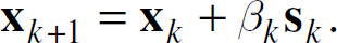
where s
k
is the search direction vector. The step size β
k
is chosen by minimizing an appropriate function called the merit function. The merit function measures how appropriate and feasible each
In the preceding section, a method was developed for determining estimates of λ given an estimate for the cdf. A naive approach to attaining values for π is to exploit equation (13). However, due to the nature of the hyperexponential density and the equations involved, the values for the vector a cannot be estimated accurately enough from data for computing π. The values attained for π from equation (13) are very sensitive to the values derived for
The cdf of the hyperexponential density is linear in π. In addition, the estimated cdf can be expressed in terms of the estimates for

for all 0 < x < ∞. Let


Define

leading to the following theorem.
Theorem 1. Equation (28) has a unique solution for the mixing proportions, given that the component means are known.
Proof. Equation (28) can be solved using linear least squares regression analysis, and is also a convex function (Boyd [21]). Therefore, this function has a global minimizer and has a unique solution for π.
From this theorem,
The following presents a summary of Algorithm 1, for obtaining estimates of the parameters for the hyperexponential density, given n samples of data.
Choose values for α such that each α
i
is distinct and positive. Obtain an initial estimate for λ. Compute â using a and the samples of data. Minimize Using the new estimate of
Algorithm 2
The second algorithm developed is similar to Algorithm 1 of the previous section. The essential difference in Algorithm 2 is that 2M parameters are estimated from the developed objective function. In the following subsection, the required objective function is developed.
Development of the Objective Function
As in the previous section, an approximate cdf is constructed as follows
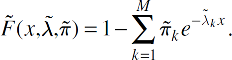
Notice that this cdf has three arguments as opposed to two, and that π is no longer described as a function of

Similarly, the approximate total error of the fit is denoted by

where m M. The function
The required parameters are obtained by minimizing the objective function in equation (31). As in the previous section, this is a constrained nonlinear optimization problem. The constraints are the same, i.e. that the component means are positive and that the mixing proportions are valid probabilities. The latter constraint can, however, be relaxed by introducing the softmax function (Bishop [20]). Let γ = {γ1, …, γ
M
} be a vector of real constants, and hence,

for all 1 i M. Fix one of γ, γ
M
(say) to be 0, which ensures that the transformation is one-to-one. Using this definition for π
i
ensures that the constraints of the mixing proportions are met. Thus, the only applicable constraint is that λ
i
> 0, for all 1 i M. However, since the hyperexponential cdf is strictly monotonic, this constraint can effectively be disregarded, reducing the problem to a nonlinear unconstrained optimization problem. Let

It is worth noticing that (33) is not a convex function of
For Algorithm 2, the only quantity that needs to be estimated is the cdf. The approach for estimating the cdf is the same in both algorithms 1 and 2. In the next subsection, a summary of the algorithm is presented.
The following presents a summary of of Algorithm 2. Estimates of the parameters of the hyperexponential density are obtained, given n samples of data.
Obtain an initial estimate for Minimize
Discussion
In this section, we discuss the expediency of the algorithms developed to sensor networks. An account of the simulation experiments executed to demonstrate the algorithms is also presented, along with a discussion of the results of these experiments.
Applicability of Algorithms to Sensor Networks
The primary strength of Algorithms 1 and 2 is that they are well-suited to sensor networks. In order to illustrate how these algorithms are applicable to sensor networks, we return to the rainfall example in section I-A. Each sensor node collects rainfall data from its immediate environment. Hansen and lnes [6] discuss the difficulties in measuring rainfall. Taking soil moisture measurements, for example, is one suggested approach for determining the amount of rainfall. However, the exact details of measuring rainfall with sensor networks are beyond the scope of this paper. The individual sensor nodes do not possess the computing power to perform the complete parameter estimation procedure. In addition, transmission of all the data values collected at all sensor nodes to the base station is impractical, as the large number of transmissions needed would quickly drain the batteries of the sensor nodes. Therefore, an algorithm such as the EM algorithm which requires all the data values would not be applicable in this scenario. Nowak [22] introduces a distribued EM algorithm approach for performing density estimation in sensor networks. In [22], it is assumed that the local processing is much less expensive than communication. We do not compare explicitly our algorithms with those in [22], since Nowak performs the density estimation of Gaussian mixtures. However, the following observations are made. In our algorithms, there is very little processing to be done at individual sensor nodes, and the number of communications for each sensor node is on par with that presented in [22]. Hence, it is expected that our algorithms will use less battery power than that of [22].
Recall that in both Algorithms 1 and 2, an estimate of the cdf of the hyperexponential density,
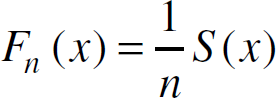
where

and u is the unit step function defined as
Only the values of Fn (x) for a fixed domain of x are required, so let the required values of x be {x1, …, xm}. Hence, the necessary values that need to be recorded and updated by each sensor node are n and S(xj) for each 1 j m. For a specific sensor node k, denote Sk to be the value of S for node k, and similarly nk denotes the value of n for node k. Each sensor node k collects data and increments its own value of nk while updating Sk. At predefined epochs, for instance when nk goes beyond a certain threshold value, the recorded values of Sk are transmitted to the base station. With this approach, each sensor node is required to record at most m+1 values. Updating and recording these values require very little computational power.
Upon transmitting the values of Sk(xj) to the base station, the sensor node resets the values of Sk(xj) for all j to zero and resets nk to zero. Each sensor node transmits m values of Sk(xj), but some values of Sk(xj) may change more often and by greater amounts than others. For instance, after a period of collecting rainfall observations we might find that Sk(x1) is large while Sk(x2) and Sk(x3) are still zero. Sending the values of just Sk(x1) would reduce the size of the transmission for node k significantly. Therefore, we propose a format for the transmission packet as in Fig. 2 . The bit vector at the head of the packet identifies which of the values of x are being sent in the packet. For instance, if bits number 1, 2, and 5 are set in the bit vector in the transmission from sensor node k, and all other bits are unset, then there are 3 data values to follow in the packet. The data values are in consecutive order and are correspondingly Sk(x1), Sk(x2) and Sk(x5). The proposed approach ensures that only values that are non-zero will be transmitted, thus minimizing the size of the transmissions.

Data packet format for transmission from sensor nodes.
The values of Sk(xj) for each sensor node k and all 1 j m, are transmitted to the base station along with the corresponding values of nk. Let
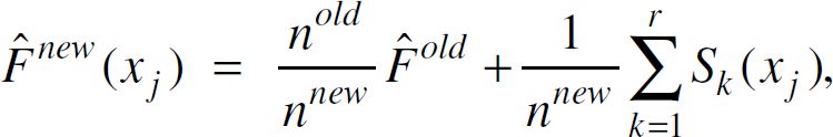
and where

If a value of Sk(xj) is not received from a sensor node, assume that it has a value of zero in equation (37).
Equation (37) is used instead of equation (21) and thus, provides the necessary estimate of the cdf in the objective functions of Algorithms 1 and 2. Once an estimate of the cdf is obtained, the base station then performs the appropriate minimization procedure to estimate the parameters of the hyperexponential density. The problem presented here of estimating the amount of rainfall in an area is ideal for sensor networks, and the approach to solving this problem is well-suited to sensor networks. Each sensor node requires only a small amount of computational power and memory, while keeping the number of network transmissions to a minimum.
The empirical cdf is commonly used as an estimator for the cdf in many applications including bootstrapping techniques and various EDF statistics such as the Cramer-von Mises and Anderson-Darling tests [23]. The virtues of the empirical cdf as an estimator stem from the fact that the empirical cdf converges uniformly to the actual cdf by the Gilvenko-Cantelli theorem [24]. Further properties of the empirical cdf are discussed extensively in [23] and [24]. The accuracy of the empirical cdf hinges on obtaining data points that range between the tails of the cdf. Extreme values which fall in the tails of the cdf will not produce good results as is the case with other estimators.
The sensor network implementation of our estimator requires the data to be discretized into several bins. The number of bins can be increased for increased accuracy. However, the final bin represents all data falling in the range [xmax, ∞). We can derive an upper bound for xmax to ensure that the probability of a random sample falling in [xmax, ∞) is below a threshold, say 1% or 0.01. Let βmax be the largest mean of all the exponential components of the mixture density. The highest probability of samples having a very large value is obtained when all other exponential components of the mixture occur with zero mixing probabilities. Therefore, we have

If we prefer this probability to be less than 0.01, we have

or, equivalently, xmax = 4.7βmax. Therefore, a good guideline is that the largest threshold in the specification of intervals for the sensor network implementation, should be about 5 times the largest anticipated mean value of the exponential probability density components of the mixture.
The Gilvenko-Cantelli theorem states that if the data samples are truly iid and the size of the data sample is sufficiently large, a good estimate of the cdf will be obtained. Since the empirical cdf is not a point estimator, deriving the standard error of the estimate is not trivial. The question of how large a sample is required for a good estimate can be answered by the Dvoretzky, Kiefer, Wolfowitz inequality [23], which is stated as follows. If X1, …, Xn are iid real-valued random variables with cdf F, and Fn is the empirical cdf, then for any d > 0 and any positive integer n.
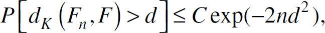
where dK is the well-known Kolmogorov-Smirnov statistic, and C is a universal constant. It can be shown that C = 2 is a good choice [23]. For illustrative purposes, if we restricted the probability of having a discrepancy of no more than 0.01 at a single point between Fn and F to be less than or equal to 0.01, then we would require approximately 200 data samples or more.
The algorithms discussed in the previous section were implemented and tested through simulation using different values for M, λ, and π. A subset of the simulation trials is discussed here. Both algorithms were tested on hyperexponential density using synthetically generated iid mixture samples. In addition, the results of both algorithms were compared to the basic implementation of the EM algorithm. Evaluation of the objective function d(λ) was performed by evaluating the approximate total error for equally spaced points over a meaningful domain. In Algorithm 1, the first phase of estimating λ is accomplished through the use of quasi-Newtonian methods with the BFGS method for the Hessian update and a safeguarded mixed quadratic and cubic polynomial interpolation and extrapolation method for line scarches. The implementation chosen is the fminunc MATLAB function [25]. For the second phase of Algorithm 1, constrained linear regression was performed using SQP methods and specifically the lsqlin MATLAB function. Algorithm 2 was implemented using quasi-Newtonian methods with the BFGS update formula, and a safeguarded mixed quadratic and cubic polynomial interpolation and extrapolation method for line searches. Once again, the fminunc MATLAB function [25] was employed.
The following is an outline of the simulation strategy utilized. In the first class of experiments, 50 experiments were performed using simulation data generated from a four component hyperexponential density having the following characteristics: λ = [1.0, 2.0, 3.0, 4.0] and
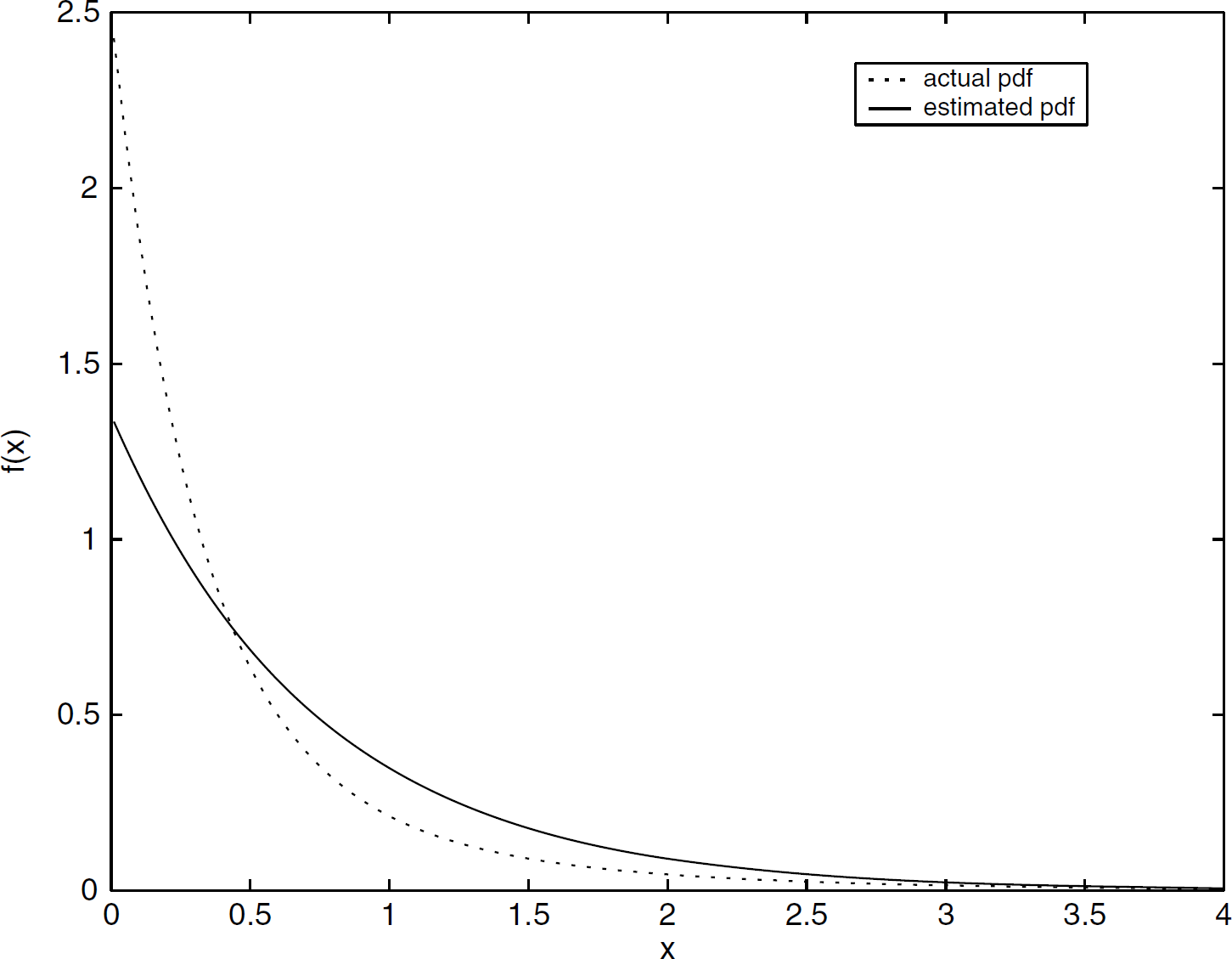
Sample results of the three algorithms are given in Figs. 3, 4, and 5. Each figure compares the generated pdf of the corresponding algorithm to the actual pdf. Each of the algorithms terminated in 1–10 iterations. From the simulation results, all of the three algorithms appear to produce similar results. In most cases, Algorithm 1 and the EM algorithm give similar results, and Algorithm 2 gives slightly better results in some cases. There is no simulation evidence to suggest that there are operating regions in which one algorithm is superior to the other, given the current approaches taken for optimization. Extensive simulation evidence indicates that Algorithm 2 gives the best results. in terms of accuracy of results, amongst the three algorithms compared.
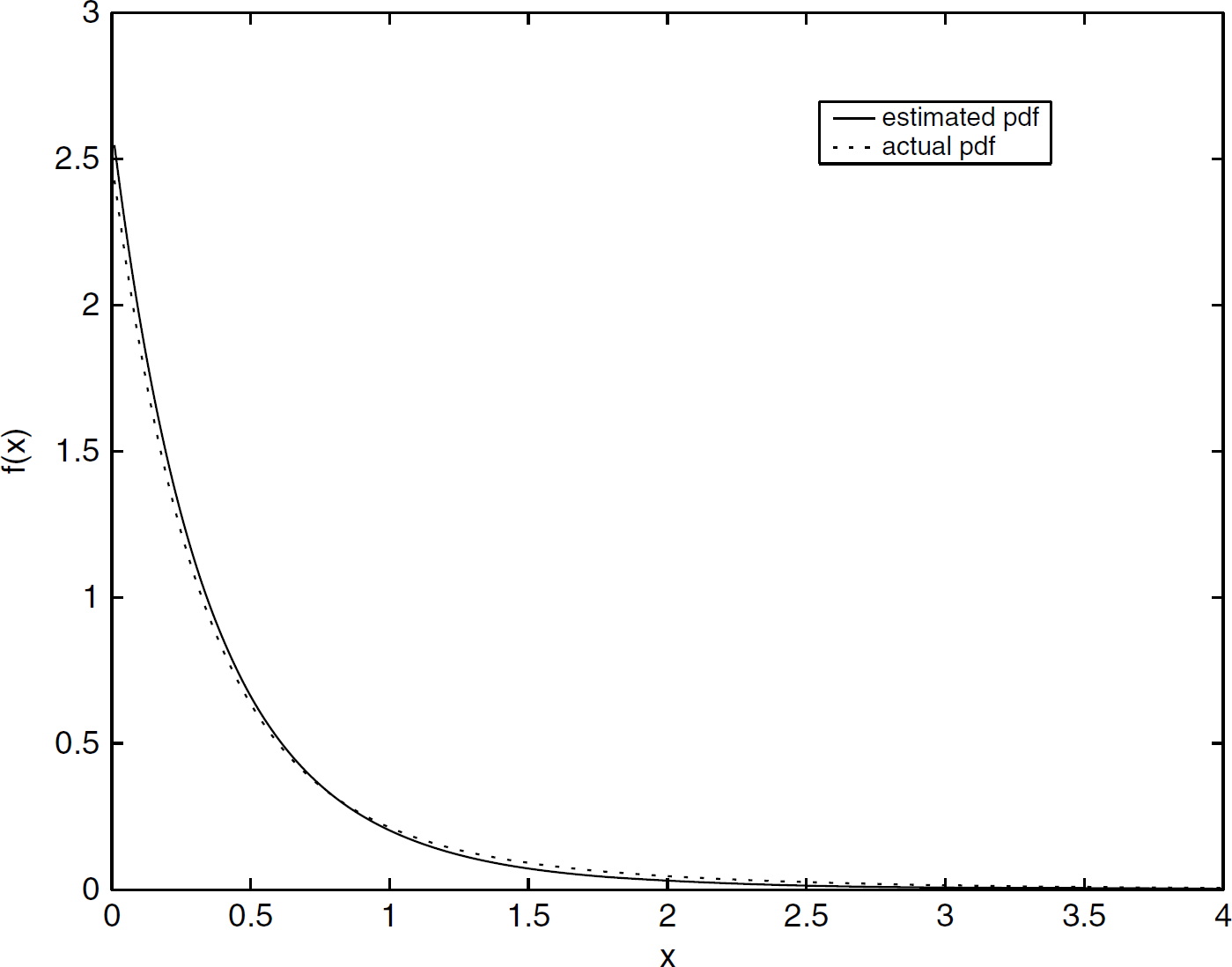
Sample plot of pdf generated from Algorithm 1 using 100 samples of data.

Sample plot of pdf generated from Algorithm 2 using 100 samples of data.
Sample plot of pdf generated from the EM algorithm using 100 samples of data.
In terms of computation speed. Algorithms 1 and 2 offer significant advantages over the EM algorithm. The EM algorithm involves computations that include all N data samples per iteration. As a consequence, as the number of data samples increases, the computation time increases dramatically. Compare this to Algorithms 1 and 2, in which the computation time of each iteration increases as a function of the number of unknown parameters only. For Algorithms 1 and 2, the values obtained from the estimated cdf function are at predefined points, and need only be looked up once, and not for every iteration. This lookup is very cheap as well, since a binary search of running time O(log N) is all that is required. For these reasons, the computation times for both Algorithms 1 and 2 are significantly improved versus the EM algorithm, particularly when N is large and the algorithms converage slowly.
The EM algorithm is generally regarded as the standard technique for estimating the parameters of mixtures of probability densities. Ruhe [26], Hasselblad [27], and Jewell [28] present solutions for finding the parameters of positive sums of exponentials, by maximum-likelihood techniques. Gruet et al [29] present a technique for estimation of mixtures of exponentials based on MCMC methods. It is well-known that the EM algorithm has a slow rate of convergence and may converge to values on the boundary of the parameter space. Moreover, the EM algorithm is not well-suited to an application in sensor networks, as the algorithm would require a high amount of network traffic to transfer all the data.
The major contributions presented here are algorithms for computing the parameters of a hyperexponential density. Our algorithms are easily implemented yet computationally very efficient. There are numerous potential applications of this algorithm particularly in the areas of network traffic modeling and queuing theory; however, the algorithms presented here are particularly applicable in sensor network situations. In particular, due to the formulation of Algorithms 1 and 2, accurate estimates of the hyperexponential pdf are obtained while keeping computation and network transmissions at the sensor nodes to a minimum. The two developed algorithms as well as the EM algorithm all give very good estimates of the hyperexponential pdf. However, extensive simulation evidence demonstrates that Algorithm 2 gives the best numerical results of the three algorithms compared, in terms of the quality of the estimate of the hyperexponential pdf produced, which is what our goal is. In addition, evidence is presented to suggest that the algorithms developed are superior to the EM algorithm in terms of computation speed in cases where a large number of data samples are present or if the convergence speed of the algorithm declines. Both algorithms developed are efficient and easily implemented using standard tools of numerical optimization.