The parameter estimation algorithms based on the dynamical response measurement data

Abstract

This article studies the parameter estimation to the system response from the discrete measurement data. By constructing the dynamical rolling cost functions and using the nonlinear optimization, the gradient identification method is presented for estimating the parameters of the sine response signal with double frequency. In order to overcome the difficulty for determining the step size and deduce the influence of noises, the stochastic gradient identification method is derived to estimate the signal parameters. For the purpose of improving the accuracy, a multi-innovation stochastic gradient parameter estimation algorithm is presented using the moving window data. Finally, the simulation examples are provided to test the algorithm performance.

Introduction

System identification and parameter estimation have been used widely in process control, signal modeling, communication, and electronic technology. The objective of parameter estimation is to obtain the parameter estimates of system models or signal models.^1–3 In general, the parameter estimation algorithm can be derived by defining and minimizing a cost function based on the measurement data.^4–6 The optimization method is one of the critical factors for parameter estimation algorithm. Many optimization methods are used in system identification and parameter estimation. Li et al. ⁷ considered the parameter estimation algorithms for Hammerstein output error systems using Levenberg–Marquardt optimization method. Xu et al. ⁸ presented a parameter estimation method based on the Newton optimization. Ding et al. ⁹ studied the least squares iterative identification algorithm for multivariate pseudo-linear autoregressive moving average (ARMA) systems. Wang and Xun ¹⁰ considered a recursive least squares identification for a class of nonlinear multiple-input single-output systems. Wang et al. ¹¹ suggested a maximum likelihood estimation method for dual-rate Hammerstein systems. All in all, different identification methods can be derived by means of different optimization. For the linear problem, the least squares method is effective. However, for the nonlinear problem, we must use the nonlinear optimization.^12,13

System identification is to obtain the system models. The system model is the basis of system control.^14–16 For a control system, the system responses contain the abundant information of the system parameters. The system response at the discrete time can be collected by means of measurement instruments. In process control, the system response is obtained by applying some typical signals. In system identification, the impulse signal, the step signal, and the sine signal are used widely to generate the measurement data for estimating system parameters. Many identification methods have been presented based on the impulse response experiment, the step response experiment, and the frequency response experiment. Ahmed et al. ¹⁷ studied the identification method from step responses with transient initial conditions. Fedele ¹⁸ considered a method to estimate a first-order plus time-delay model from the step response. Xu and Ding ¹⁹ presented a damping iterative parameter identification method for dynamical systems based on the sine signal. Hidayat and Medvedev ²⁰ studied the Laguerre domain identification of continuous linear time-delay systems from impulse response data. This article studies the parameter estimation based on the response signals.

The accuracy, the computation complexity, and the robustness^21–23 are main aspects of the identification algorithm performance.^24,25 Many identification algorithms focus on enhancing the accuracy and robust and reducing the complexity.^26–28 Wang and Ding^29–31 considered the filtering algorithm to reduce the algorithm’s complexity. Mao and Ding ³² used the filtering technique to the Hammerstein controlled autoregressive systems to reduce the complexity. Na et al. ³³ studied the robust adaptive finite-time parameter estimation for robotic systems. Increasing the measurement data used in the estimation computation is an effective method.^34,35 Moreover, some methods based on the model decomposition or the parameter decomposition can reduce the complexity.^36,37 Wang and colleagues^38,39 suggested the hierarchical estimation algorithms to reduce the complexity. Wang and colleagues^40,41 considered a multi-innovation parameter estimation method for Hammerstein nonlinear system to enhance the accuracy. The objective of this article is to propose the identification algorithms to obtain high accuracy and low complexity. In system identification, the recursive computation and the iterative computation are used to obtain the parameter estimates.^42–45 Wang and Ding^46,47 studied the recursive identification algorithm for nonlinear systems. Xu ⁴⁸ proposed the iterative Newton method to estimate the system parameters from step response. Wang and Ding ⁴⁹ studied a recursive parameter and state estimation algorithm for the input nonlinear state space system. In general, the recursive computation can use the online data; therefore, the recursive algorithm can be used in the online identification.

The rest of this article is organized as follows. Section “Problem description” describes the identification and estimation problem from the system response. Section “The recursion gradient identification algorithm” derives the gradient identification method. Section “The SG identification method based on the dynamical data” derives the stochastic gradient (SG) parameter estimation method. Section “The multi-innovation stochastic gradient identification based on the moving window data” derives the multi-innovation gradient parameter estimation method. Section “Examples” gives some examples to illustrate the performance of the proposed methods. Finally, section “Conclusion” gives some concluding remarks.

Problem description

In process control, the linear time-invariant system can be described by the transfer function $G(s)$ . The system modeling is to obtain the system parameters. This problem is called parameter estimation. In fact, it is difficult to achieve the system parameters directly. The system response is the system output by applying some excitation signals. The impulse signal, the step signal, and the sine signal are used widely as the excitation signals in the practical engineering. The excitation signals are the input signals. Once these signals are applied to the system to be modeled, the systems can generate the responses. Therefore, the system responses contain the system characteristic information. In order to obtain the system parameters, we can use the system response information to derive the parameter estimation algorithm. Then, the parameter estimates can be obtained using the parameter estimation algorithms.

Let $R(s)$ denote the Laplace transform of the input; let $Y(s)$ denote the Laplace transform of the output; let $y(t)$ denote the system response. According to the definition of the transfer function, we have $Y(s)=G(s)R(s)$ . The system response $y(t)$ is the inverse Laplace transform, that is, $y(t)=L^{-1}[G(s)R(s)]$ . For a process control system, different input signals lead to different responses, such as the impulse response, the step response, and the frequency response. In general, for the transfer function $G(s)$ , the system response is a function containing exponential terms or sine terms. Therefore, the response $y(t)=f(\mathit{\theta },t)$ is a highly nonlinear function with respect to the system parameters $\mathit{\theta }$ . This nonlinear form causes difficulties for estimating the system parameters based on the response measurement data. Moreover, the identification algorithm can be realized by means of constructing and minimizing the cost function about the system parameters. In order to obtain the system parameter estimates, the problem of minimizing the cost function is converted to the nonlinear optimization.

The measurement data contain the parameter information. The use of the measurement data is an important factor for identification method. Suppose that the sampling time is $t_k$ . As a result, the measurement data are represented as $y(t_1),y(t_2),\dots$ . The values of the response function at the sampling time $t_k$ are $f(\mathit{\theta },t_1),f(\mathit{\theta },t_2),\dots$ . Because the measurement data contain the measurement noise, the measurement output is not equal to the response model output. If the model output is very close to the measurement output, the model is effective for describing the system characteristic. The model structure and parameter are the components of the system model. After the model structure is determined, the model parameters are obtained by the parameter estimation method. According to the different measurement data which are used in the algorithm, we can construct different cost functions. For the single data $y(t_k)$ at time $t_k$ , the cost function can be defined as

$$J(\mathit{\theta }):=\frac{1}{2}[y(t_k)-f(\mathit{\theta },t_k){]}^2$$

(1)

For a batch of measurement data $y(t_k),y(t_{k-1}),\dots ,y(t_{k-p+1})$ , where $p$ is the data length of the batch data, define the cost function based on the batch data

$$J(\mathit{\theta }):=\frac{1}{2}\sum _{j=k-p+1}^k[y(t_j)-f(\mathit{\theta },t_j){]}^2$$

(2)

From the cost functions, we can see that the cost functions are the rolling optimization function with the change of the sampling time. So the real-time measurement data can be used to estimate system parameters. The purpose of this article is to propose the parameter estimation based on the nonlinear dynamical rolling optimization and the discrete response measurement data.

The recursion gradient identification algorithm

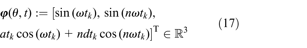
Consider a response of a combinatorial sine signal

$$\hat{y}(t)=a\sin (\omega t)+d\sin (n\omega t)$$

(3)

where $a$ and $d$ are the amplitude, $\omega$ is the angular frequency, and $n$ is a constant.

Suppose that the observation time is $t_k,k=1,2,\dots$ . The measurement data at time $t_k$ are $y(t_k)$ . In practical, the measurement data $y(t_k)$ at time $t_k$ contain the measured error. Therefore, the measurement data $y(t_k)$ are not equal to the model output $\hat{y}(t_k)$ . Define the difference between the model output and the measurement output as

$$\begin{array}{c}\multicolumn{1}{c}{v(t_k):=y(t_k)-\hat{y}(t_k)}\\ =y(t_k)-a\sin (\omega t_k)-d\sin (n\omega t_k)\hfill \end{array}$$

(4)

If the error is very small, it means that the signal model is satisfied. This problem can be converted into minimizing the gradient cost function. Define the parameter vector $\mathit{\theta }:=[a,d,\omega {]}^{\mathrm{T}}\mathbb{R}{\in }^3$ . Define the cost function

$$\begin{array}{c}\multicolumn{1}{c}{J_1(\mathit{\theta }):=J_1(a,d,\omega )=\frac{1}{2}{v}^2(t_k)}\\ =\frac{1}{2}{[y(t_k)-a\sin (\omega t_k)-d\sin (n\omega t_k)]}^2\hfill \end{array}$$

(5)

Because the measurement data $y(t_k)$ vary with the sampling time $t_k$ , the observation data in the cost function $J_1(\mathit{\theta })$ vary with the sampling time. Therefore, the dynamical measurement data are used in the cost function $J_1(\mathit{\theta })$ . The parameter estimates $\hat{\mathit{\theta }}(t_k)$ at time $t=t_k$ can be obtained by minimizing $J_1(\mathit{\theta })$ .

Taking the first-order derivative of $J_1(\mathit{\theta })$ with respect to $\mathit{\theta }$ , we can obtain the gradient vector

$$\mathrm{grad}[J_1(\mathit{\theta })]:=\frac{\partial J_1(\mathit{\theta })}{\partial \mathit{\theta }}={[\frac{\partial J_1(\mathit{\theta })}{\partial a},\frac{\partial J_1(\mathit{\theta })}{\partial d},\frac{\partial J_1(\mathit{\theta })}{\partial \omega }]}^{\mathrm{T}}\in {\mathbb{R}}^3$$

(6)

$$\frac{\partial J_1(\mathit{\theta })}{\partial a}=-\sin (\omega t_k)[y(t_k)-a\sin (\omega t_k)-d\sin (n\omega t_k)]$$

(7)

$$\frac{\partial J_1(\mathit{\theta })}{\partial d}=-\sin (n\omega t_k)[y(t_k)-a\sin (\omega t_k)-d\sin (n\omega t_k)]$$

(8)

$$\begin{array}{c}\multicolumn{1}{c}{\frac{\partial J_1(\mathit{\theta })}{\partial \omega }=-[a{t}_k\cos (\omega t_k)+\mathrm{nd}{t}_k\cos (n\omega t_k)]}\\ \times [y(t_k)-a\sin (\omega t_k)-d\sin (n\omega t_k)]\hfill \end{array}$$

(9)

Let $\hat{\mathit{\theta }}(t_k):=[\hat{a}(t_k),\hat{d}(t_k),\hat{\omega }(t_k){]}^{\mathrm{T}}$ be the estimates of $\mathit{\theta }$ at time $t=t_k$ , that is, the parameter estimates at the recursion $k$ . According to the negative gradient search and minimizing the cost function $J_1(\mathit{\theta })$ , the gradient (also called the least mean square (LMS) algorithm) for estimating the sine signal with double frequency is given by

$$\hat{\mathit{\theta }}(t_k)=\hat{\mathit{\theta }}(t_{k-1})-\mu (t_k)\mathrm{grad}[J_1(\hat{\mathit{\theta }}(t_{k-1}))]$$

(10)

$$\begin{array}{c}\mathrm{grad}[J_1(\hat{\mathit{\theta }}(t_{k-1}))]\hfill \\ ={[\frac{\partial J_1(\hat{\mathit{\theta }}(t_{k-1}))}{\partial a},\frac{\partial J_1(\hat{\mathit{\theta }}(t_{k-1}))}{\partial b},\frac{\partial J_1(\hat{\mathit{\theta }}(t_{k-1}))}{\partial \omega }]}^{\mathrm{T}}\hfill \end{array}$$

(11)

$$\begin{array}{c}\frac{\partial J_1(\hat{\mathit{\theta }}(t_{k-1}))}{\partial a}=-\sin (\hat{\omega }(t_{k-1})t_k)\hfill \\ [y(t_k)-\hat{a}(t_{k-1})\sin (\hat{\omega }(t_{k-1})t_k)-\hat{d}(t_{k-1})\sin (n\hat{\omega }(t_{k-1})t_k)]\hfill \end{array}$$

(12)

$$\begin{array}{c}\frac{\partial J_1(\hat{\mathit{\theta }}(t_{k-1}))}{\partial d}=-\sin (n\hat{\omega }(t_{k-1})t_k)[y(t_k)\hfill \\ -\hat{a}(t_{k-1})\sin (\hat{\omega }(t_{k-1})t_k)-\hat{d}(t_{k-1})\sin (n\hat{\omega }(t_{k-1})t_k)]\hfill \end{array}$$

(13)

$$\begin{array}{l}\frac{\partial J_1(\widehat{\mathit{\theta }}(t_{k-1}))}{\partial \omega }=-[\widehat{a}(t_{k-1})t_k\cos (\widehat{\omega }(t_{k-1})t_k)+n\widehat{d}(t_{k-1})t_k\cos (\widehat{\omega }(t_{k-1})t_k)]\\ \times [y(t_k)-\widehat{a}(t_{k-1})\sin (\widehat{\omega }(t_{k-1})t_k)-\widehat{d}(t_{k-1})\sin (n\widehat{\omega }(t_{k-1})t_k)]\end{array}$$

(14)

$$\mu (t_k)=\underset{\mu \ge 0}{\mathrm{argmin}}{J}_1(\hat{\mathit{\theta }}(t_{k-1})-\mu \mathrm{grad}[J_1(\hat{\mathit{\theta }}(t_{k-1}))])$$

(15)

The steps of computing the parameter estimates $\hat{\mathit{\theta }}(t_k)$ using the recursion gradient (RG) identification algorithm (10)–(15) are as follows:

1. To initiate: let $k=1$ ; let $\hat{\mathit{\theta }}(t_0)=[\hat{a}(t_0),\hat{d}(t_0),\hat{\omega }(t_0){]}^{\mathrm{T}}\in {\mathbb{R}}^3$ be an real vector;

2. Collect the measurement data $y(t_k)$ ;

3. Compute the terms of the gradient using equations (12)–(14); form the gradient vector $[J_1(\hat{\mathit{\theta }}(t_{k-1}))]$ using equation (11);

4. Compute the step size $\mu (t_k)$ using equation (15);

5. Compute the parameter estimates $\hat{\mathit{\theta }}(t_k)$ using equation (12);

6. Increase $k$ by 1 and go to Step (2).

Remark 1

The step size $\mu (t_k)$ at each recursion can be determined by the one-dimensional search. However, it is very difficult to obtain the step size by the direct equation solving. We can use the cut-and-try method to determine the step size or use the optimization method such as the Newton iterative method and the gradient method.

The SG identification method based on the dynamical data

The gradient parameter estimation algorithm needs to optimize the step size at each recursion $k$ . For the sine response signal, it is complicated to obtain the step size using one-dimensional search. With the increasing of the recursion, the step size cannot trend to zero. Therefore, the algorithm is sensitive to the noise. In order to avoid sensitivity to the noise and in order to avoid the complicated computation to determine the step size, we present the SG algorithm parameter estimation method. This algorithm can determine the step size automatically at each recursion.

Define the cost function based on the dynamical data

$$J_2(\mathit{\theta }):=\frac{1}{2}{[y(t_k)-a\sin (\omega t_k)-d\sin (n\omega t_k)]}^2$$

(16)

Define the information vector

$$\begin{array}{c}\mathit{\phi }(\theta ,t):=[\sin (\omega t_k),\sin (n\omega t_k),\hfill \\ a{t}_k\cos (\omega t_k)+\mathrm{nd}{t}_k\cos (n\omega t_k){]}^{\mathrm{T}}\in {\mathbb{R}}^3\hfill \end{array}$$

(17)

Then, the gradient of the cost function $J_2(\mathit{\theta })$ can be represented as

$$\mathrm{grad}[J_2(\mathit{\theta })]=-\mathit{\phi }(\mathit{\theta },t_k)[y(t_k)-a\sin (\omega t_k)-d\sin (n\omega t_k)]$$

(18)

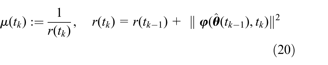
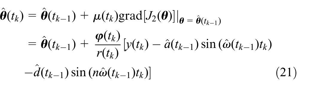
Let $\hat{\mathit{\theta }}(t_k):=[\hat{a}(t_k),\hat{d}(t_k),\hat{\omega }(t_k)]$ be the recursive parameter estimate of the parameter vector $\mathit{\theta }$ at the recursion $k$ . Then, we have

$$\begin{array}{c}\mathrm{grad}[J_2(\mathit{\theta })]{|}_{\mathit{\theta }=\hat{\mathit{\theta }}(t_{k-1})}=\mathrm{grad}[J_2(\hat{\mathit{\theta }}(t_{k-1}))]\hfill \\ =-\mathit{\phi }(\hat{\mathit{\theta }}(t_{k-1}),t_k)[y(t_k)-\hat{a}(t_{k-1})\sin (\hat{\omega }(t_{k-1})t_k)\hfill \\ -\hat{d}(t_{k-1})\sin (n\hat{\omega }(t_{k-1})t_k)]\hfill \end{array}$$

(19)

In order to reduce the sensitivity to the noise, the step size $\mu (t_k)$ is set to

$$\mu (t_k):=\frac{1}{r(t_k)},r(t_k)=r(t_{k-1})+\parallel \mathit{\phi }(\hat{\mathit{\theta }}(t_{k-1}),t_k){\parallel }^2$$

(20)

Based on the negative gradient search and minimizing the cost function $J_2(\mathit{\theta })$ , we can obtain the SG algorithm for estimating the sine response

$$\begin{array}{c}\multicolumn{1}{c}{\hat{\mathit{\theta }}(t_k)=\hat{\mathit{\theta }}(t_{k-1})+\mu (t_k)\mathrm{grad}[J_2(\mathit{\theta }{)]|}_{\mathit{\theta }=\hat{\mathit{\theta }}(t_{k-1})}}\\ =\hat{\mathit{\theta }}(t_{k-1})+\frac{\mathit{\phi }(t_k)}{r(t_k)}[y(t_k)-\hat{a}(t_{k-1})\sin (\hat{\omega }(t_{k-1})t_k)\hfill \\ -\hat{d}(t_{k-1})\sin (n\hat{\omega }(t_{k-1})t_k)]\hfill \end{array}$$

(21)

$$r(t_k)=r(t_{k-1})+\parallel \mathit{\phi }(\hat{\mathit{\theta }}(t_{k-1}),t_k){\parallel }^2,r(t_0)=1$$

(22)

$$\begin{array}{c}\hat{\mathit{\phi }}(t_k)=[\sin (\hat{\omega }(t_{k-1})t_k),\sin (n\hat{\omega }(t_{k-1})t_k),\hfill \\ \hat{a}(t_{k-1})t_k\cos (\hat{\omega }(t_{k-1})t_k)+n\hat{d}(t_{k-1})t_k\cos (n\hat{\omega }(t_{k-1})t_k){]}^{\mathrm{T}}\hfill \end{array}$$

(23)

$$\mathit{\theta }(t_k)=[\hat{a}(t_k),\hat{d}(t_k),\hat{\omega }(t_k)]$$

(24)

The steps of computing the parameter estimates $\hat{\mathit{\theta }}(t_k)$ using the gradient identification algorithm (equations (21)–(24)) are as follows:

1. To initiate: let $k=1$ ; let $\hat{\mathit{\theta }}(t_0)=[\hat{a}(t_0),\hat{d}(t_0),\hat{\omega }(t_0){]}^{\mathrm{T}}\in {\mathbb{R}}^3$ be an real vector; pre-set the recursive length $L_e$ ;

2. Collect the measurement data $y(t_k)$ ;

3. Compute the information $\hat{\mathit{\phi }}(t_k)$ using equation (23);

4. Compute $r(t_k)$ using equation (22);

5. Compute the parameter estimates $\hat{\mathit{\theta }}(t_k)$ using equation (21);

6. If $k=L_e$ , terminate the recursive process and obtain the characteristic parameters from equation (24); otherwise, increase $k$ by 1 and go to Step (2).

Remark 2

The method of determining the step size $\mu (t_k)$ between the gradient method and the SG method is different. For the SG method, the step size $\mu (t_k)$ is set using the information vector. It can update automatically with the increasing recursion $k$ .

The multi-innovation stochastic gradient identification based on the moving window data

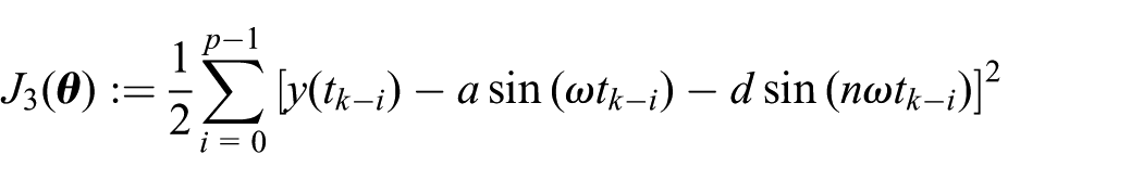
The gradient identification algorithm and the SG algorithm use the current data at the sampling time $t_k$ . Only one step data is used, and the accuracy is low. In order to enhance the estimation accuracy, we use the batch data in the latest time to construct the cost function. For system identification algorithm, the more the measurement data is used, the higher the estimation accuracy is. However, too many measurement data used in the algorithm can lead to the heavy computation complexity. Therefore, we propose to use the moving window measurement data to derive the parameter estimation algorithm.

The moving window measurement data are a batch data, and they can update dynamically. The moving window data are represented as $y(t_k),y(t_{k-1}),\dots ,y(t_{k-p+1})$ , where $p$ is the length of the moving window. Based on the moving window data and the multi-innovation theory, ⁵⁰ we derive the parameter identification algorithm for the sine signal with double frequency.

Define the cost function $J_3(\mathit{\theta })$ using the moving window data

$$J_3(\mathit{\theta }):=\frac{1}{2}\sum _{i=0}^{p-1}[y(t_{k-i})-a\sin (\omega t_{k-i})-d\sin (n\omega t_{k-i}){]}^2$$

Taking the first-order derivative of $J_3(\mathit{\theta })$ with respect to $\mathit{\theta }=[a,d,\omega {]}^{\mathrm{T}}$ , the gradient vector is given by

$$\mathrm{grad}[J_3(\mathit{\theta })]:=\frac{\partial J_3(\mathit{\theta })}{\partial \mathit{\theta }}={[\frac{\partial J_3(\mathit{\theta })}{\partial a},\frac{\partial J_3(\mathit{\theta })}{\partial d},\frac{\partial J_3(\mathit{\theta })}{\partial \omega }]}^{\mathrm{T}}\in {\mathbb{R}}^3$$

(25)

$$\begin{array}{c}\multicolumn{1}{c}{\frac{\partial J_3(\mathit{\theta })}{\partial a}=-\sum _{i=0}^{p-1}[y(t_{k-i})-a\sin (\omega t_{k-i})-d\sin (n\omega t_{k-i})]}\\ \sin (\omega t_{k-i})\hfill \end{array}$$

(26)

$$\begin{array}{c}\multicolumn{1}{c}{\frac{\partial J_3(\mathit{\theta })}{\partial d}=-\sum _{i=0}^{p-1}[y(t_{k-i})-a\sin (\omega t_{k-i})-d\sin (n\omega t_{k-i})]}\\ \sin (n\omega t_{k-i})\hfill \end{array}$$

(27)

$$\begin{array}{c}\multicolumn{1}{c}{\frac{\partial J_3(\mathit{\theta })}{\partial \omega }=-\sum _{i=0}^{p-1}[y(t_{k-i})-a\sin (\omega t_{k-i})-d\sin (n\omega t_{k-i})]}\\ [a{t}_{k-i}\cos (\omega t_{k-i})+\mathrm{nd}{t}_{k-i}\cos (n\omega t_{k-i})]\hfill \end{array}$$

(28)

Define the information vector

$$\mathit{\phi }(\mathit{\theta },t_k):=[\sin (\omega t_k),\sin (n\omega t_k),a\cos t_k(\omega t_k)+\mathrm{nd}\cos (\omega t_k){]}^{\mathrm{T}}\in {\mathbb{R}}^3$$

Define the information matrix based on the window data

$$\mathbf{\Phi }(p,\mathit{\theta },t_k):=[\mathit{\phi }(\mathit{\theta },t_k),\mathit{\phi }(\mathit{\theta },t_{k-1}),\dots ,\mathit{\phi }(\mathit{\theta },t_{k-p+1})]\in {\mathbb{R}}^{3\times p}$$

Let $\hat{\mathit{\theta }}(t_k):=[\hat{a}(t_k),\hat{d}(t_k),\hat{\omega }(t_k)]$ be the estimate of the parameter vector $\mathit{\theta }$ at time $t=t_k$ . Define the scalar innovation: $e(\hat{\mathit{\theta }}(t_{k-1}),t_k):=y(t_k)-\hat{a}(t_{k-1})\sin (\hat{\omega }(t_{k-1})t_k)-\hat{d}(t_{k-1})\sin (n\hat{\omega }(t_{k-1})t_k)$ . Expanding the scalar innovation $e(\hat{\mathit{\theta }}(t_{k-1}),t_k)\in \mathbb{R}$ into the innovation vector gives

$$\begin{array}{c}\multicolumn{1}{c}{\mathit{E}(p,t_k):=\left[\begin{array}{c}e(\hat{\mathit{\theta }}(t_{k-1}),t_k)\hfill \\ \multicolumn{1}{c}{e(\hat{\mathit{\theta }}(t_{k-1}),t_{k-1})}\\ \multicolumn{1}{c}{⋮}\\ \multicolumn{1}{c}{e(\hat{\mathit{\theta }}(t_{k-1}),t_{k-p+1})}\end{array}\right]}\\ =\left[\begin{array}{c}y(t_k)-\hat{a}(t_{k-1})\sin (\hat{\omega }(t_{k-1})t_k)-\hat{d}(t_{k-1})\sin (n\hat{\omega }(t_{k-1})t_k)\hfill \\ \multicolumn{1}{c}{y(t_{k-1})-\hat{a}(t_{k-1})\sin (\hat{\omega }(t_{k-1})t_{k-1})-\hat{d}(t_{k-1})\sin (n\hat{\omega }(t_{k-1})t_{k-1})}\\ \multicolumn{1}{c}{⋮}\\ \multicolumn{1}{c}{y(t_{k-p+1})-\hat{a}(t_{k-1})\sin (\hat{\omega }(t_{k-1})t_{k-p+1})-\hat{d}(t_{k-1})\sin (n\hat{\omega }(t_{k-1})t_{k-p+1})}\end{array}\right]\hfill \\ =\mathit{Y}(p,t_k)-{\mathit{F}}_1(p,t_k)-{\mathit{F}}_2(p,t_k)\hfill \end{array}$$

(29)

$$\mathit{Y}(p,t_k)=[y(t_k),y(t_{k-1}),\dots ,y(t_{k-p+1}){]}^{\mathrm{T}}\in {\mathbb{R}}^p$$

(30)

$$\begin{array}{c}{\mathit{F}}_1(p,t_k)=[\hat{a}(t_{k-1})\sin (\hat{\omega }(t_{k-1})t_k),\hfill \\ \hat{a}(t_{k-1})\sin (\hat{\omega }(t_{k-1})t_{k-1}),\dots ,\hat{a}(t_{k-1})\hfill \\ \sin (\hat{\omega }(t_{k-1})t_{k-p+1}){]}^{\mathrm{T}}\in {\mathbb{R}}^p\hfill \end{array}$$

(31)

$$\begin{array}{c}\multicolumn{1}{c}{{\mathit{F}}_2(p,t_k)=[\hat{d}(t_{k-1})\sin (n\hat{\omega }(t_{k-1})t_k),}\\ \multicolumn{1}{c}{\hat{d}(t_{k-1})\sin (n\hat{\omega }(t_{k-1})t_{k-1}),\dots ,\hat{d}(t_{k-1})}\\ \sin (n\hat{\omega }(t_{k-1})t_{k-p+1}){]}^{\mathrm{T}}\in {\mathbb{R}}^p\hfill \end{array}$$

(32)

Using the negative gradient search and minimizing the cost function $J_3(\mathit{\theta })$ , the multi-innovation stochastic gradient (MISG) algorithm is given by

$$\begin{array}{c}\multicolumn{1}{c}{\hat{\mathit{\theta }}(t_k)=\hat{\mathit{\theta }}(t_{k-1})-\frac{1}{r(t_k)}\mathrm{grad}[J_3(\hat{\mathit{\theta }}(t_{k-1}))]}\\ =\hat{\mathit{\theta }}(t_{k-1})+\frac{\hat{\mathbf{\Phi }}(p,t_k)}{r(t_k)}\mathit{E}(p,t_k)\hfill \end{array}$$

(33)

$$\mathit{E}(p,t_k)=\left[\begin{array}{c}y(t_k)-\hat{a}(t_{k-1})\sin (\hat{\omega }(t_{k-1})t_k)-\hat{d}(t_{k-1})\sin (n\hat{\omega }(t_{k-1})t_k)\hfill \\ \multicolumn{1}{c}{y(t_{k-1})-\hat{a}(t_{k-1})\sin (\hat{\omega }(t_{k-1})t_{k-1})-\hat{d}(t_{k-1})\sin (n\hat{\omega }(t_{k-1})t_{k-1})}\\ \multicolumn{1}{c}{⋮}\\ \multicolumn{1}{c}{y(t_{k-p+1})-\hat{a}(t_{k-1})\sin (\hat{\omega }(t_{k-1})t_{k-p+1})-\hat{d}(t_{k-1})\sin (n\hat{\omega }(t_{k-1})t_{k-p+1})}\end{array}\right]$$

(34)

$$r(t_k)=r(t_{k-1})+\parallel \hat{\mathbf{\Phi }}(p,t_k){\parallel }^2,r(t_0)=1$$

(35)

$$\begin{array}{c}\hat{\mathbf{\Phi }}(p,t_k)=\mathbf{\Phi }(p,\hat{\mathit{\theta }}(t_{k-1}),t_k)\hfill \\ =[\mathit{\phi }(\hat{\mathit{\theta }}(t_{k-1}),t_k),\mathit{\phi }(\hat{\mathit{\theta }}(t_{k-1}),t_{k-1}),\dots ,\mathit{\phi }(\hat{\mathit{\theta }}(t_{k-1}),t_{k-p+1})]\hfill \\ =[\hat{\mathit{\phi }}(t_k),\hat{\mathit{\phi }}(t_{k-1}),\dots ,\hat{\mathit{\phi }}(t_{k-p+1})]\hfill \end{array}$$

(36)

$$\begin{array}{c}\multicolumn{1}{c}{\hat{\mathit{\phi }}(t_{k-i})=\mathit{\phi }(\hat{\mathit{\theta }}(t_{k-1}),t_{k-i})}\\ =[\sin (\hat{\omega }(t_{k-1})t_{k-i}),\sin (n\hat{\omega }(t_{k-1})t_{k-i}),\hfill \\ \hat{a}(t_{k-1})t_{k-i}\cos (\hat{\omega }(t_{k-1})t_{k-i})+n\hat{d}(t_{k-1})t_{k-i}\hfill \\ \cos (n\hat{\omega }(t_{k-1})t_{k-i}){]}^{\mathrm{T}},i=0,1,\dots ,p-1\hfill \end{array}$$

(37)

$$\hat{\mathit{\theta }}(t_k)=[\hat{a}(t_k),\hat{d}(t_k),\hat{\omega }(t_k)]$$

(38)

The steps of computing the parameter estimates using the MISG algorithm (equations (33)–(38)) are as follows:

1. To initiate: let $k=1$ ; pre-set the innovation length $p$ ; let $\hat{\mathit{\theta }}(t_0)=[\hat{a}(t_0),\hat{d}(t_0),\hat{\omega }(t_0)]$ be a real vector; let $r(t_0)=1$ . Pre-set the recursive length $L_e$ ;

2. Collect the measurement data $y(t_k)$ . Compute and construct the information vector $\hat{\mathit{\phi }}(t_{k-i}),i=0,1,\dots ,p-1$ using equation (37). Form the stack matrix $(\hat{\mathbf{\Phi }}p,t_k)$ using equation (36);

3. Compute $r(t_k)$ using equation (35). Compute the innovation vector $(p,t_k)$ using equation (34);

4. Update the parameter estimates $\hat{\mathit{\theta }}(t_k)$ using equation (33). Obtain the estimates of the characteristic parameters $\hat{a}(t_k)$ , $\hat{d}(t_k)$ , and $\hat{\omega }(t_k)$ from $\hat{\mathit{\theta }}(t_k)$ using equation (38);

5. If $k=L_e$ , terminate the recursive process; otherwise, $k:=k+1$ and go to Step (2).

Remark 3

The MISG method is derived on the basis of the SG method by expanding the scalar innovation into the innovation vector using the moving window measurement data. The moving window data update with the recursion $k$ dynamically. The scheme of the moving window data make more data to participate in the recursive estimation computation. It can improve the estimation accuracy.

Examples

In this section, we provide some examples to show the performance of the proposed method.

Example 1

Consider a power signal

$$y(t)=5\sin (2t)+10\sin (4t)$$

where the true values are $a=5$ , $d=10$ , and $\omega =2$ .

In the simulation, the white noise is applied to the response signal. The noise variance is ${\sigma }^2=0.{10}^2$ , ${\sigma }^2=0.{80}^2$ , and ${\sigma }^2=2.{00}^2$ . Using the proposed RG method to estimate the response parameters, the parameter estimates and their estimation errors $\delta :=\parallel {\hat{\mathit{\theta }}}_k-\mathit{\theta }\parallel /\mathit{\theta }$ are shown in Table 1. The estimation errors $\delta$ versus $k$ are shown in Figure 1.

Table 1.

The RG estimates and estimation errors.

${\sigma }^2$	$k$	$a$	$d$	$\omega$	$\delta$ (%)
$0.{10}^2$	5	5.99699	11.99699	2.90912	20.78537
	10	5.98910	11.98911	2.83020	20.43685
	20	5.97690	11.97694	2.76322	20.08543
	50	5.55476	11.56861	2.36928	14.50865
	100	4.89302	10.97619	2.28766	8.77658
	200	4.62401	10.74657	2.27957	7.60596
	400	5.15293	10.81028	2.27966	7.51556
	600	5.03696	10.82366	2.27966	7.51475
$0.{80}^2$	5	5.99688	11.99688	2.92257	20.82673
	10	5.98973	11.98974	2.85813	20.52884
	20	5.98466	11.98468	2.82768	20.37081
	50	5.56719	11.57979	2.38064	14.65151
	100	4.97040	11.04183	2.30159	9.29974
	200	4.58357	10.74612	2.29354	7.79463
	400	5.16766	10.82690	2.29367	7.70886
	600	5.02444	10.84434	2.29367	7.71654
$2.{00}^2$	5	5.99670	11.99671	2.94562	20.89880
	10	5.99080	11.99081	2.90598	20.69168
	20	5.99797	11.99795	2.93829	20.88882
	50	5.58861	11.59908	2.39947	14.89849
	100	5.10329	11.15457	2.32473	10.30981
	200	4.51425	10.74540	2.31673	8.14811
	400	5.19292	10.85543	2.31693	8.04617
	600	5.00297	10.87984	2.31693	8.06935
True values		5.00000	10.00000	2.00000

RG: recursion gradient.

Figure 1.

The RG parameter estimation errors $\delta$ versus $k$ .

Example 2

Consider a power signal with double frequency

$$y(t)=2\sin (5t)+3\sin (15t)$$

where the true values are $a=2$ , $d=3$ , and $\omega =5$ .

In the simulation, the white noise is applied to the response signal. In order to test the sensitivity to the noise, the noise variance is taken as ${\sigma }^2=0.{50}^2$ and ${\sigma }^2=4.{00}^2$ , respectively. The ratio of the variance is 8. Using the proposed SG method to estimate the parameters of the power signal in Example 2, the parameter estimates and their estimation errors $\delta :=\parallel {\hat{\mathit{\theta }}}_k-\mathit{\theta }\parallel /\mathit{\theta }$ are shown in Table 2. The estimation errors $\delta$ versus $k$ are shown in Figure 2.

Table 2.

The SG estimates and estimation errors.

$k$	$a$	$d$	$\omega$	$\delta$ (%)
1	2.17973	3.24120	4.65368	7.44126
5	2.17142	3.22462	4.58170	8.18873
10	2.17042	3.22450	4.62856	7.56393
20	2.17067	3.22367	4.67715	6.94695
30	2.17059	3.22361	4.68529	6.84691
50	2.17056	3.22360	4.69062	6.78246
100	2.17055	3.22359	4.68915	6.79994
1	2.18881	3.26753	5.03265	5.33818
5	2.17103	3.23313	4.91726	4.87875
10	2.16979	3.23267	4.97627	4.68840
20	2.16924	3.23136	4.97683	4.66529
30	2.16911	3.23126	4.98486	4.65399
50	2.16906	3.23121	4.99371	4.64754
100	2.16903	3.23120	4.98966	4.64897
True values	2.00000	3.00000	5.00000

SG: stochastic gradient.

Figure 2.

The SG parameter estimation errors $\delta$ versus $k$ .

Example 3

Consider a power signal with double frequency

$$y(t)=8\sin (0.5t)+3\sin (t)$$

where the true values are $a=8$ , $d=3$ , and $\omega =0.5$ .

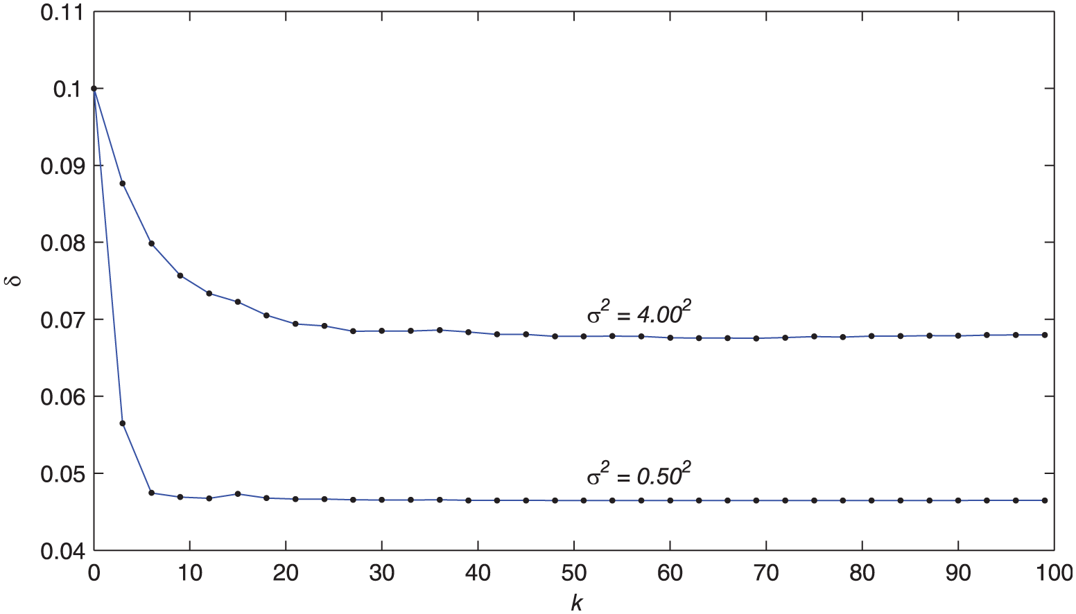
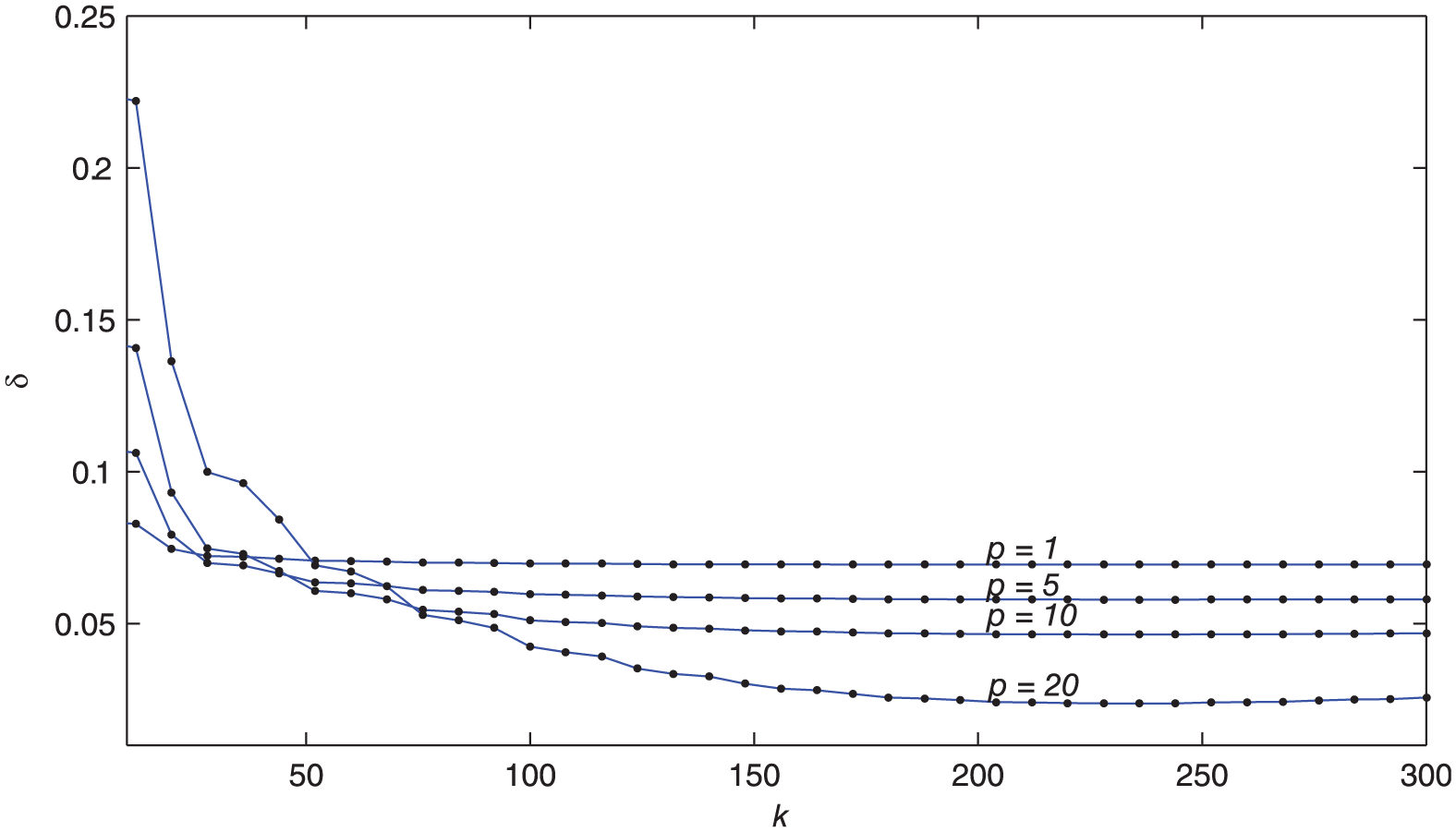
In the simulation, the dynamical data with different innovation lengths $p=1$ , $p=5$ and $p=9$ are used to estimate the response parameters. The recursion length is $L_e=300$ . The variance of the white noise is ${\sigma }^2=4.{00}^2$ . Using the proposed MISG method to estimate the signal parameters, the parameter estimates and their estimation errors $\delta :=\parallel {\hat{\mathit{\theta }}}_k-\mathit{\theta }\parallel /\mathit{\theta }$ for different $p$ are shown in Table 3. The estimation errors $\delta$ versus $k$ for different $p$ are shown in Figure 3.

Table 3.

The MISG estimates and estimation errors.

$p$	$k$	$a$	$d$	$\omega$	$\delta$ (%)
1	5	7.44140	2.78157	0.05408	8.73253
	10	7.44425	2.77984	0.06366	8.64720
	50	7.44828	2.77983	0.38174	7.07687
	100	7.44832	2.77984	0.43586	6.98053
	150	7.44833	2.77983	0.46594	6.95156
	200	7.44833	2.77983	0.48631	6.94204
	250	7.44833	2.77982	0.50131	6.94025
	300	7.44832	2.77982	0.51286	6.94190
5	5	7.52281	2.82715	−0.38684	11.93881
	10	7.52850	2.82367	−0.36768	11.72066
	50	7.53656	2.82367	0.26848	6.39399
	100	7.53665	2.82367	0.37671	5.96902
	150	7.53666	2.82366	0.43689	5.83930
	200	7.53666	2.82365	0.47762	5.79851
	250	7.53665	2.82365	0.50762	5.79337
	300	7.53665	2.82364	0.53072	5.80387
10	5	7.60421	2.87272	−0.82775	16.25640
	10	7.61275	2.86751	−0.79901	15.91338
	50	7.62485	2.86750	0.15522	6.15136
	100	7.62497	2.86751	0.31757	5.11276
	150	7.62499	2.86750	0.40783	4.77032
	200	7.62498	2.86748	0.46893	4.66142
	250	7.62498	2.86747	0.51392	4.65022
	300	7.62497	2.86746	0.54858	4.68202
20	5	7.76701	2.96387	−1.70959	25.96369
	10	7.78126	2.95518	−1.66169	25.39185
	50	7.80141	2.95517	−0.07131	7.08639
	100	7.80162	2.95519	0.19928	4.24171
	150	7.80164	2.95516	0.34972	2.95448
	200	7.80164	2.95514	0.45156	2.44271
	250	7.80163	2.95512	0.52654	2.39653
	300	7.80162	2.95510	0.58431	2.57260
True values		8.00000	3.00000	0.50000

MISG: multi-innovation stochastic gradient.

Figure 3.

The MISG parameter estimation errors $\delta$ versus $k$ .

From the simulation results, we can draw the following conclusive remarks:

• The common feature of the proposed RG method, the SG method, and the MISG method is that the estimation errors reduce with the increasing of the recursion $k$ . This implies that the proposed methods are effective for estimating the response parameters.

• The simulation results in Example 1 show that the RG method is sensitive to the noise. The variety curves of the parameter estimates shake seriously. The changing curves of the parameter estimates given by the SG method from Example 2 show that the variety of the estimation errors obtained by the SG method has no serious fluctuation when the noise variance is big.

• The estimation accuracy given by the MISG method changes with the increasing of the innovation length $p$ (i.e. the moving window data length). The innovation length denotes the numbers of measurement data participated in the recursion computation. If the innovation length is big, the estimation accuracy is high.

• Compared the proposed three methods, the MISG method can obtain more satisfactory effectiveness than the RG method and the SG method. Even though the RG method and the SG method have low accuracy, their computation complexity is low.

Conclusion

This article considers the parameter estimation problem to the system response from the discrete measurement data. Using the dynamical measurement data and the moving window measurement data, the RG method, the SG method, and the MISG method are presented for estimating the response parameters. The simulation results show that the proposed algorithms are effective. The proposed methods can be expanded to parameter estimation of speech signal processing,^51,52 the self-organizing map, ⁵³ and applied to other fields.^54–65